Highlights
What are the main findings?
- An automated workflow was developed to generate geometrically consistent urban CFD meshes from open-source data.
- CFD simulations of Ourense reveal complex wind patterns and regions of high turbulence, validated through experimental measurements using anemometers.
What is the implication of the main findings?
- The methodology enables reliable prediction of urban wind fields without requiring proprietary or high-cost 3D city models.
- The generated CFD outputs can be integrated into UAV trajectory optimisation frameworks to enhance flight safety and efficiency in urban areas.
Abstract
Turbulence and wind gusts pose significant risks to the safety and efficiency of UAVs (uncrewed aerial vehicles) in urban environments. In these settings, wind dynamics are strongly influenced by interactions with buildings and terrain, giving rise to small-scale phenomena such as vortex shedding and gusts. These wind speed oscillations generate unsteady forces that can destabilise UAV flight, particularly for small vehicles. Additionally, predicting their formation requires high-resolution Computational Fluid Dynamics (CFD) models, as current weather forecasting tools lack the resolution to capture these phenomena. However, such models require 3D representations of study areas with high geometric consistency and detail, which are not available for most cities. To address this issue, this work introduces an automated methodology for urban CFD mesh generation using open-source data. The proposed method generates error-free meshes compatible with OpenFOAM and includes tools for geometry modification, enhancing solver convergence and enabling adjustments to mesh complexity based on computational resources. Using this approach, CFD simulations are conducted for the city of Ourense, followed by an analysis of their impact on UAV operations and the integration of the system into a trajectory optimisation framework. The CFD model is also validated using experimental anemometer measurements.
1. Introduction
In recent years, UAV (uncrewed aerial vehicle) operations have expanded rapidly due to their cost-effectiveness and high maneuverability [1,2,3]. These advantages have sparked growing interest in deploying UAVs for urban logistics, particularly for last-mile delivery. This concept involves using UAVs for short-distance transport as an alternative to traditional ground vehicles, enhancing delivery efficiency while reducing the environmental impact of transportation [4,5,6]. Operations would be highly autonomous and coordinated from logistics hubs. At these hubs, such as vertiports, UAVs could be recharged and reloaded. These services would operate within an Urban Air Mobility (UAM) framework, granting operators access to air traffic management, communication systems, and real-time airspace information to ensure safe and efficient operations [7].
Despite their societal benefits, UAV operations entail significant risks, as any incident could compromise the safety of other airspace users and people on the ground [8]. New technologies are therefore required to mitigate the risks associated with unexpected events. One major factor to consider is the impact of urban wind patterns [9]. The interaction of wind with buildings and other urban structures can lead to wake formation and vortex shedding, producing high-frequency wind speed fluctuations [10]. These fluctuations generate unsteady aerodynamic forces and torques, which can destabilise UAV control, particularly for smaller vehicles [11,12]. Although several control strategies have been proposed in recent years to reduce the impact of wind gusts on UAV attitude and trajectory tracking [13,14], efficiently predicting and avoiding these hazardous areas remain crucial for safe operations [15].
Accurately predicting these phenomena is challenging, as they typically occur at scales of a few metres and require high-resolution microweather data [16,17]. Computational Fluid Dynamics (CFD) tools can be employed to locally refine wind predictions based on regional meteorological forecasts. Typically, forecasted conditions are used to adjust CFD inflow profiles, such as the Atmospheric Boundary Layer (ABL), after which CFD simulations are run to improve the accuracy and resolution of the resulting wind fields.
Among the most common CFD approaches, it is worth mentioning (1) Large Eddy Simulation (LES) methods, which resolve the largest energy-containing turbulent eddies while modelling only the subgrid-scale motions. These methods offer high fidelity for unsteady separated and wake flows that govern transient gusts affecting small aerial vehicles [18,19]. However, their spatial and temporal resolution requirements make them computationally expensive and thus practical only for small domains encompassing a few buildings. In contrast, (2) Reynolds-Averaged Navier–Stokes (RANS) methods solve time-averaged equations using turbulence models [20,21]. Although they do not directly resolve the turbulent eddies, their accuracy is reasonably good, with errors relative to the LES of the order of 10%, while maintaining much lower computational costs. This efficiency allows their application to larger domains, such as extensive urban areas [22].
However, such simulations require detailed models of urban geometry, which are not readily available for many cities. Furthermore, due to the complex geometry of urban settings, manual 3D modelling is time-consuming and often infeasible [23,24]. In this regard, NASA’s CFD Vision 2030 identifies geometry preparation as the main bottleneck of CFD-based systems, highlighting the importance of automated processing tools [25]. Although there are numerous open-source urban 3D datasets, most are designed for 3D visualisation purposes, making them unsuitable for CFD mesh generation because of low geometric consistency and existing errors (missing surfaces and non-manifold edges) [26,27]. Previous works proposed geometry repair methodologies, but this remains a manual and labour-intensive process [28]. Recent studies have introduced automated methodologies to produce geometries free of such errors, merging building footprints from cadastral data with LiDAR or photogrammetry point clouds. However, incorporating all these elements into CFD models may be impractical due to substantial resource requirements. Consequently, establishing frameworks for model simplification has become another key challenge [29,30].
Another common challenge is integrating terrain models into urban geometry to prevent gaps and intersections, which can cause problems in mesh generation. For this reason, some studies simplify the problem by modelling the ground surface as a plane [31,32]. However, this approach is only suitable for cities with relatively flat terrain, as in areas with significant elevation changes, this simplification yields unrealistic results [33,34]. Recent research has developed watertight integration methods, incorporating roughness layers to account for varying terrain textures [23,35]. While these methods enable CFD-compatible mesh generation, they can introduce convergence issues in CFD solvers. For instance, steep slopes near the computational domain boundaries may trigger flow separations and wakes, leading to fluctuations and numerical instability. Therefore, alongside 3D modelling, geometry treatment techniques are essential to ensure simulation convergence [30].
Another key factor is vegetation’s impact on wind flow, commonly modelled as a porous medium, adding terms to flow equations that account for pressure and momentum losses in these areas [36,37]. Due to vegetation’s complex geometry, automated volume modelling techniques are applied, such as LiDAR point clouds [38], but most face limitations in accurately characterising different vegetation types [39].
To address all listed limitations, this study presents a comprehensive and flexible 3D modelling methodology for developing CFD-based microweather systems. The proposed tool uses open-source data to generate finite volume meshes adaptable to the available computational resources and the characteristics of the study area. Using this approach, the wind patterns of an urban area are simulated and the results are experimentally validated using anemometers. The main contributions of this work are as follows:
- Enhanced terrain model integration: The proposed approach is specifically designed for areas with significant elevation changes and steep slopes. In addition to producing error-free geometries, a new geometry-smoothing method is introduced to prevent wakes near the computational domain boundaries, ensuring numerical stability.
- Development of adaptive geometry modelling tools: The proposed framework includes tools to adjust the geometric level of detail according to available computational resources. It introduces a novel method for implicit building modelling based on porosity models. This low-detail approach considers the effects of these elements on wind flow without increasing mesh complexity, making it particularly useful for large-scale simulations.
- Suitability analysis of a preliminary microweather system for vertiport operations: The developed CFD model was coupled with a mesoscale weather forecast to obtain high-resolution wind predictions. Using this approach, a probabilistic evaluation was conducted to quantify the prediction uncertainties.
2. Methodology
2.1. The 3D Geometric Model Generation
2.1.1. Area of Study Definition
The urban area of Ourense, a city of around 100,000 inhabitants in northwestern Spain, is selected as a case study. Since no last-mile delivery services currently operate in the area, a hypothetical scenario is proposed, placing a vertiport at the Faculty of Aerospace Engineering at the University of Vigo. For the simulations, a circular area with a radius of 1 km centred on this building is considered, as shown in Figure 1b. For the 3D reconstruction, data from the Spanish Geographic Institute (IGN) is used, as it is the official national institution and provides high-quality geospatial data. However, the proposed methodology is fully adaptable to other countries, as most provide similar data through their respective national geographic institutes, or, alternatively, high-quality geospatial data can be obtained from international open-source repositories [40].
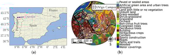
Figure 1.
Geographical location and land use map of the area for the conceptual vertiport environment in Ourense, Spain. (a) Location of Ourense, a city with approximately 100,000 inhabitants in northwestern Spain. (b) SIOSE AR map of the area. This product represents the land usage of the area of study according to the Spanish Geographic Institute (IGN) [41].
2.1.2. Terrain Geometry
To generate the 3D model, the terrain geometry is created using the Digital Elevation Model (DEM) MDT05 from the Spanish Geographic Institute (IGN), shown in Figure 2a. It consists of a regularly spaced grid in UTM coordinates with a 5 m horizontal resolution, accurately mapping terrain elevation. The city of Ourense features significant elevation changes, making it necessary to include the DEM in the CFD and to consider a large domain to account for topographic effects on wind currents. To prevent numerical instabilities caused by flow separation at the boundaries of the domain [30], an artificial domain extension is added to the geometry, following the height profile outlined in Figure 2b. For this purpose, a polar coordinate system is employed, where r represents the radial distance from the centre of the domain, and denotes the azimuthal angle. Two zones are defined:
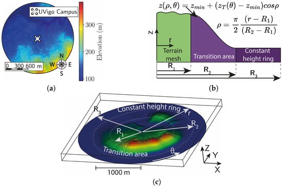
Figure 2.
Terrain 3D model generation process using Digital Elevation Models from IGN [41]. (a) Elevation Model MDT05 [41]. (b) Height profile scheme of the buffer area. (c) Terrain 3D model including the buffer area.
- Transition area (): This provides a smooth elevation transition between the terrain mesh and the constant height ring, using a cosine elevation profile (Figure 2b). It spans from the limits of the terrain mesh ( = 1 km) to the constant height ring ( = 1.6 km). This last value was chosen based on the recommendations from An et al. [42], which suggest avoiding slopes steeper than 30° near the domain boundaries. With this configuration, the maximum slope is 22°, considering for steepest case of the variable.
- Constant height ring (): A flat surface with a constant elevation equal to the minimum terrain height (). Its purpose is to ensure organised inflow and outflow. It extends up to a radius of 2 km.
2.1.3. Land Semantic Classification
To characterise terrain roughness properties, the SIOSE AR model from IGN is used [41], a vector map that classifies surfaces across the Spanish territory into categories. To expedite processing, the map is converted to a 5 m resolution raster format (Figure 1b) and the mesh triangles are then classified based on their centroid positions, resulting in the categorised 3D model shown in Figure 3.
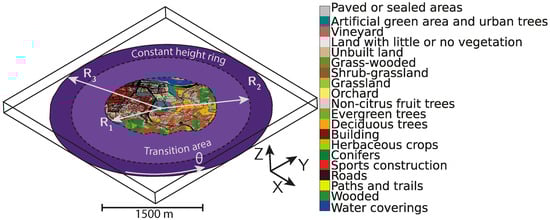
Figure 3.
Semantically classified terrain geometry using SIOSE AR product [41].
2.1.4. Buildings’ Geometry
The level of detail and complexity of 3D building models must be balanced based on the available computational resources. Two Levels of Detail (LoDs), based on Biljecki et al.’s [43] building categorisation, are considered here:
- LoD 1.3: Buildings are represented as simple blocks with flat roofs.
- LoD 2.1: Simplified roof elevation variations are included, excluding fine details.
Models with higher LoDs not only increase simulation complexity but are challenging to reconstruct and require very high-resolution geospatial data [29]. In this work, LiDAR point clouds from IGN are used, which have a spatial density of 0.5 points/—insufficient for capturing these fine details. This low resolution can lead to issues such as self-intersections or non-manifold edges. Therefore, to produce error-free surfaces, we combine LiDAR data with SIOSE AR building footprints derived from cadastral data. The reconstruction process, shown in Figure 4, comprises the following steps:
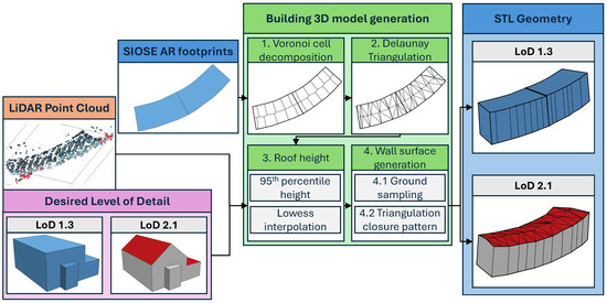
Figure 4.
Building geometry generation workflow diagram using IGN open-source data [41].
- Voronoi cell decomposition: Building footprints are decomposed into convex polygons using Voronoi cells from boundary points, fully covering the domain.
- Delaunay triangulation: Applied to each Voronoi cell to create a 2D surface without gaps or overlaps.
- Roof height calculation: Roof heights are derived from IGN LiDAR point clouds. Points within the ground floor polygon are extracted, and heights are assigned to Delaunay points according to LoD:
- LoD 1.3: Roofs are modelled as flat surfaces at the 95th percentile height of the point cloud.
- LoD 2.1: Roofs are modelled through a Lowess interpolation, adjusted with point cloud heights.
- Wall surface generation: Building side walls are created from the roof’s outer points. Terrain height is sampled, and an extrusion is performed, closing the building volume with a triangulation pattern.
2.1.5. Geometry Simplification
The study area spans 3 and contains several thousand buildings. Including all structures in CFD simulations would drastically increase the number of mesh elements, leading to impractical memory and computational demands. A trade-off between model complexity and computational feasibility is therefore necessary, focusing on buildings that most strongly influence wind flow in the vertiport area around the UVigo campus within a radius of m (Figure 5a). Only buildings with a direct line of sight from the vertiport and a footprint exceeding 750 are geometrically modelled, primarily excluding the single-family homes in the domain’s eastern sector. This simplification follows Blocken’s CFD urban modelling guidelines [30]. These guidelines recommend omitting urban features whose sizes are comparable to the cell size, as they have limited influence on domain-scale wind patterns and would require very fine local mesh refinement to capture near-surface velocity profiles. The 750 cutoff was selected after examining the domain geometries to ensure that all buildings with a substantial effect on wind flow were retained.
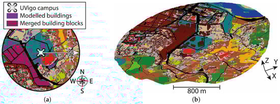
Figure 5.
Building model simplification and integration into the terrain surface. (a) High-detail area definition. (b) Simplified building geometry.
Additionally, the geometry of the building blocks southwest of the campus is simplified following the LoD 1.3 specification. Buildings within each block are merged, with the ground floor reduced to a single exterior polygon parallel to the surrounding roads, while features such as inner courtyards are omitted. This process is performed automatically by processing the SIOSE AR map polygons corresponding to each building block. The resulting simplified geometric model of the area of interest is shown in Figure 5b.
2.2. CFD Wind Simulation
2.2.1. CFD Mesh Generation
The computational domain is created in Ansys SpaceClaim 2023, defined by a cylinder with a radius of km and a height range of m. The terrain surface is imported, and a boolean operation is applied to remove the volume below it (Figure 6). The CFD mesh is generated using the polyHexCore method in Ansys Fluent Meshing, employing a terrain surface element size of 2.5 m. Larger elements are used for outer surfaces (), while a minimum cell size of 1.5 m is applied to the volumetric mesh to accommodate complex geometries. The cell size is further reduced in the study area to capture air dynamics in detail. Boundary layers are generated over the terrain and geometrically modelled buildings to achieve acceptable values: on terrain and on buildings. In this way a mesh comprising 34 million cells is obtained. The mesh is finally exported to OpenFOAM 10, and a cell ordering operation is performed to reduce the matrix bandwidth for numerical solvers.
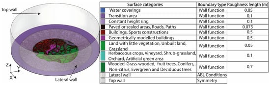
Figure 6.
Computational domain. For the boundary conditions, roughness lengths are adjusted based on the results of Silva et al. [44].
2.2.2. Vegetation and Urban Structures Modelling
Vegetation and structures outside the largest building areas are modelled as porous media. For buildings not explicitly modelled, a cell zone is created to encompass all mesh cells within their volumes. Following the procedure outlined in Section 2.1.4, the corresponding building volumes are generated, and the enclosed cells are extracted. For vegetation areas, point clouds from IGN are used [41], identified as red points in Figure 7. To accelerate data processing, the point clouds are first voxelised into a structured 2D mesh representing terrain areas occupied by vegetation. Next, the vegetation height in each occupied voxel is computed as the 95th percentile of the point cloud’s height. Elements with centroids within an occupied voxel and heights lower than the vegetation height are classified as vegetation volumes. Finally, the cells are categorised according to the SIOSE AR model, and a cellzone is created for each vegetation type.
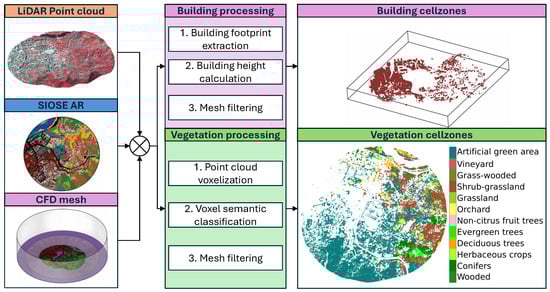
Figure 7.
Vegetation and urban structure cellzone calculation using IGN open-source data [41].
2.2.3. Boundary Conditions
For boundary conditions (Figure 8), wall effects are considered using a nutk wall function with variable roughness parameters, adjusted based on Silva et al. [44]. Symmetry conditions are imposed on the top wall, while an Atmospheric Boundary Layer (ABL) wind profile is defined for the lateral surface of the cylinder. The ABL model employs a logarithmic wind profile, adjusted by a reference velocity and wind direction at a specific reference height, (Figure 8). To fit these parameters, the CFD system is coupled with MeteoGalicia’s Weather Research and Forecasting (WRF) model, a mesoscale weather prediction system that provides wind speed and direction forecasts () at m above ground level (AGL).
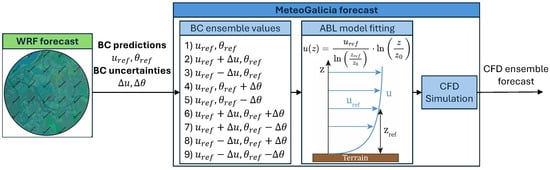
Figure 8.
CFD wind ensemble forecasting based on WRF model uncertainties [45].
However, MeteoGalicia’s predictions carry uncertainties that can significantly impact CFD results. The WRF model typically has an error of 1.6 m/s in wind speed () and in wind direction () [45]. To address these uncertainties, we evaluate nine scenarios by perturbing the boundary conditions, taking into account the typical deviations of the WRF model, as detailed in Figure 8. This method produces an ensemble CFD forecast, facilitating a probabilistic analysis of local wind conditions.
Porous media are represented using the Darcy–Forchheimer model, which adds a source term to the momentum equation, , where is the fluid viscosity, is the fluid density, and U is the fluid velocity. The parameters D and F represent viscous and inertial losses, respectively. Buildings are treated as impermeable media by assigning high loss coefficients, with and , to block fluid passage. With these values, the momentum loss is of the order of . If this term is substituted into the flow momentum equation, the spatial gradient of wind speed becomes very large, producing a rapid exponential decay along the flow direction. Defining x as the flow direction, the wind intensity profile can be approximated as
indicating an extremely fast decay that blocks the flow, as if encountering a solid obstacle.
For vegetation, inertial losses are calculated as , where LAD is the Leaf Area Density, and is the drag coefficient [46]. Values of and are used based on prior studies [47,48].
2.2.4. Simulation Setup
The wind profiles are simulated with simpleFoam, the OpenFOAM steady-state solver for incompressible flow. The k– turbulence model was used. Spatial discretisation schemes are second-order-accurate. Pressure was solved with the GAMG iterative method, and the remaining fields were solved with the smooth Gauss–Seidel solver. Two non-orthogonal corrector loops were applied, a uniform tolerance of was used, and relaxation factors were 0.8 for velocity and 0.3 for the other variables.
A mesh sensitivity analysis was performed to evaluate the effect of mesh resolution on the results. With boundary conditions and , three meshes (Table 1) were compared by examining wind speed at several probe locations around the region of interest. Deviations of Mesh 1 and Mesh 2 with respect to Mesh 3 (reference) were 6.1% and 1.3%, respectively. Simulation times were approximately 1.3, 2.0, and 7.5 h for Mesh 1, Mesh 2, and Mesh 3, respectively. Mesh 2 provided a good compromise between accuracy and computational cost.

Table 1.
Summary of meshes tested in the sensitivity analysis. Deviation is reported relative to Mesh 3 (reference).
Due to the large size and complexity of the case study, the computational cost of the current setup is significant despite using a steady-state RANS solver. The designed mesh yields typical cell sizes of about 2.5 m near ground surfaces and 1.5 m near building surfaces. If LESs were employed, cell sizes would need to be reduced to below 1 m to resolve eddies properly, implying meshes of several hundred million to billions of cells and potentially prohibitive memory and computing requirements. Given that the main contribution of this work is the modelling methodology rather than high-fidelity LES results, the RANS approach was selected.
2.3. CFD Validation
CFD results are validated through an experimental campaign, with anemometers installed at the locations highlighted in Figure 9a. All these points are selected within the high-detail zone in order to evaluate the accuracy of the model near the building of interest. Three portable Campbell Windsonic 1 anemometers are placed on the ground (Figure 9b) and configured with a sampling frequency of 1 Hz. Additionally, a fixed Campbell 05103 anemometer, installed on the rooftop of the Faculty of Aerospace Engineering, was used (Figure 9c) to provide average wind values at 10 min intervals.
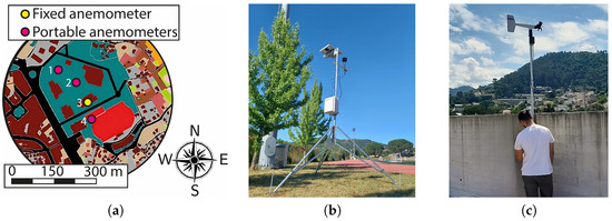
Figure 9.
Anemometers used in the experimental data acquisition campaign on 11 June 2024. (a) Anemometer positions. (b) Campbell Windsonic 1 portable anemometer. (c) Campbell 05103 anemometer installed on the rooftop of the Faculty of Aerospace Engineering. Numbers 1–4 indicate the identity of each anemometer employed.
For each hour of the experiment, the average measured wind modulus and direction are computed for each anemometer. The boundary conditions for these hours are obtained from MeteoGalicia’s WRF model (Table 2), and the CFD ensemble forecast is computed following the methodology introduced in Section 2.2. The predictions are then compared with the experimental results by extracting the CFD values at each anemometer position.
Table 2.
MeteoGalicia’s WRF model predictions on 11 June 2024 [45]. Model resolution: 1 km (horizontal) and 1 h (temporal). Wind speed and direction correspond to a reference height m above ground level. Local time in Ourense is CEST (UTC+2).
Additionally, to assess the formation of turbulence zones and vortices in the area, the variance of the x- and y-components of wind speed measurements (denoted as and ) is calculated for each time interval. These components represent the amplitude of velocity fluctuations relative to their mean values. From these, the experimental turbulence kinetic energy is determined and compared with the OpenFOAM results. It is noteworthy that these results can only be computed for the portable anemometers, as the fixed one provides wind values only at 10 min intervals, which does not allow for the assessment of wind speed fluctuations.
2.4. UAV Path Planning Application
As a practical application of the proposed methodology, the wind forecasting system is integrated into a path planning framework, using results from a previous study [49].
2.4.1. Airspace Mesh Generation
For the path planning, the computational domain is discretised into a graph structure , where V denotes the set of vertices, and E denotes the set of connecting edges. To this end, the k-NANN (k-Non-Aligned Nearest Neighbour) meshing method introduced in a previous work [49] is employed. This approach constructs a graph in which each vertex is connected to its k nearest non-aligned neighbours. The parameter k is adjustable, allowing a trade-off between computational complexity and path smoothness: higher values of k increase graph density, enabling finer vehicle control, but at the cost of greater computational effort. Figure 10a illustrates the k-NANN concept in two dimensions, showing a node connected to its 64 closest non-aligned neighbours.
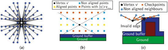
Figure 10.
Mesh generation using the k-NANN (k-Non-Aligned Nearest Neighbour) approach [49]. (a) 2D representation of 64 k-NANN. (b) Flight path angle constraints. (c) Ground buffer constraints.
To avoid excessive climb rates and ensure smooth trajectories, the vehicle’s flight path angle is constrained to a maximum value of . Edges for which exceeds this threshold are removed from the graph (Figure 10b). Additionally, to maintain a minimum clearance from urban structures, a ground separation buffer of m is imposed on all edges. To evaluate this condition, a set of evenly spaced checkpoints is defined along each edge , with a spacing of 5 m between consecutive points. At each checkpoint, the distance to the surrounding urban geometry is assessed (Figure 10c), and edges that violate this constraint are discarded.
This process ensures that all connections in the graph are flyable and compliant with operational requirements, thereby reducing the need for constraint checking during the planning phase and decreasing the overall computation time. In this study, a three-dimensional uniform mesh with a resolution of 10 m and a value of are used.
2.4.2. Path Planner
For the trajectory calculation, an path-planning approach is employed, as outlined in Algorithm 1. First, the arrival cost () and the estimated cost to the destination () are initialised for all nodes in the graph (). All and values are initially set to infinity, except for those of the starting node, which is added to a binary priority queue. An iterative exploration process is then performed, in which, at each step, the node with the lowest estimated cost to the destination, , is extracted from the queue. All neighbouring nodes of are subsequently explored, provided they satisfy the following operational constraints:
- Heading angle constraint: To avoid abrupt changes in direction, a maximum allowable variation in heading angle of is established. For each edge connecting node to its neighbour , the heading angle difference is computed, where corresponds to the heading angle of edge , and corresponds to that of the preceding edge arriving at node .
- Turbulent kinetic energy (k) constraint: Based on the CFD results, k is evaluated at all checkpoints along each edge (Figure 10c). Only those edges for which k remains below a predefined threshold, , are considered traversable by the UAV, following a similar approach to that of Gu et al. [50].
| Algorithm 1 Trajectory optimiser algorithm. |
|
For each neighbour that satisfies these constraints, a new candidate arrival cost, , is computed and compared with the previous arrival cost, . If the former is lower, the node cost is updated, and the estimated cost to reach the neighbour is given by , where denotes the Euclidean distance between nodes. The priority of in the queue is then adjusted accordingly. This process continues until the destination node () is reached, at which point the search terminates and the optimal trajectory is returned.
3. Results
3.1. CFD Simulation Results
Figure 11 shows the horizontal wind profiles at different altitudes above mean sea level (AMSL) during the hour of peak wind intensity on 11 June 2024. These results are based on the nominal WRF forecast values ( m/s, ). Pronounced velocity gradients are observed across the four altitude levels, primarily due to substantial terrain elevation changes and the presence of buildings. The strongest winds, reaching 8 m/s, occur in the northeast at 190 m above sea level, where the airflow is less obstructed. This wind speed approaches the operational limits of some commercial UAV models [51], and the presence of turbulence and gusts further increases flight risks.
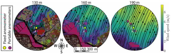
Figure 11.
Wind predictions for 11 June 2024 at 15:00 UTC, using the nominal values from the WRF forecast ( m/s, ). Each subplot represents the horizontal wind speed and direction at different altitudes above mean sea level (AMSL). Altitude values are selected based on the terrain elevation of the area. Numbers 1–4 indicate the anemometer numbering from Figure 9.
In contrast, the wind speed in the southwest drops to near zero due to buildings that obstruct airflow. Figure 11 shows the effects of porosity as introduced in Section 2.2.2. Although buildings are not geometrically modelled, this method effectively approximates their impact, improving predictions near anemometers. Figure 12 further illustrates this effect in a cross-sectional plane () along the main wind direction (). High-porosity zones modelling buildings reduce wind speed and create realistic velocity gradients and wakes. The figure also displays the domain extensions introduced in Section 2.1.2, which ensure orderly inflow and outflow despite the significant elevation changes.
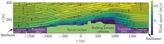
Figure 12.
Cross-sectional cut of the computational domain on a vertical plane () aligned with the reference wind direction = 22.04°. The figure showcases the vertical wind profiles obtained for 11 June 2024 at 15:00 UTC. Reported altitudes are reported with respect to mean sea level (AMSL).
Figure 13 presents the turbulence kinetic energy (k) for the same hour of study. Similar to wind speed, the highest k values appear in the northeast, where the flow has greater convective energy. Despite being a sparsely built area, the significant slopes and elevation changes contribute to the formation of wakes and areas of turbulence. The highest values for k occur at 190 m above sea level, reaching 10 J/kg, which corresponds to an average wind speed fluctuation of 4.47 m/s, posing a risk to UAM operations.

Figure 13.
Turbulence kinetic energy (k) predictions for 11 June 2024 at 15:00 UTC, using the nominal values from the WRF forecast ( m/s, ). Each subplot represents the value of this magnitude at different altitudes above mean sea level (AMSL). Altitude values are selected based on the terrain elevation of the area. Numbers 1–4 indicate the anemometer numbering from Figure 9.
3.2. CFD Validation
Figure 14 compares CFD results with experimental wind measurements, highlighting that wind speed predictions at the four anemometers carry notable uncertainty (around 2 m/s) due to WRF errors. Reasonable correlations are found, as all measurements fall within the confidence intervals and all errors are below 1 m/s. The CFD model generally overestimates wind speeds; however, predictions at 14:00 and 18:00 UTC are closest to actual values, reflecting instances where the reference velocity from MeteoGalicia aligns more accurately with true conditions.
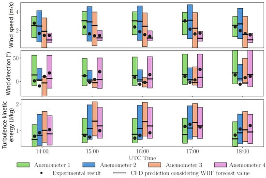
Figure 14.
Comparison between simulations and experimental measurements from the anemometers. Points indicate the experimental measurements. Lines indicate the CFD prediction using MeteoGalicia’s forecast values (). Boxes consider the confidence interval of the ensemble forecast, considering the uncertainties in boundary conditions. Anemometer numbers refer to the numbering introduced in Figure 9. Anemometer 3’s turbulence kinetic energy is not reported, as this device only provides average wind properties at 10 min intervals.
The uncertainty in direction spans approximately 60°, primarily due to the WRF model’s typical angular deviation of 35°, which widens the gap between CFD predictions and measurements, with errors reaching up to 20°. Some experimental values lie outside the confidence interval, but, considering the 1 − error from the WRF ensemble forecast, this outcome is expected as only 68% of predictions should fall within this range, assuming a Gaussian error distribution. For turbulent kinetic energy, all measurements fall within CFD confidence intervals, with deviations below 0.5 J/kg. Despite the RANS model’s lack of explicit turbulence eddy dissipation, the average wind speed oscillations predicted by the k– model align reasonably well with experimental data.
Table 3 summarises the errors for each hour by averaging results from all anemometers. It displays the mean absolute error and the bias, calculated as the average of the errors including their signs. Significant variations are observed at different measurement times. At 14:00 and 18:00 UTC, the CFD model’s wind speed deviates least from experimental results, with bias values of 0.25 and 0.04 m/s, suggesting that the WRF model’s values are closer to actual conditions. Conversely, at 16:00 UTC, the wind direction bias reaches a minimum of 0.3°, indicating improved accuracy in predicting the average wind direction (better value).
Table 3.
CFD errors considering nominal values from the WRF forecast. Each cell represents the average difference between experiments and simulations considering the four anemometers. Mean error is the average absolute error (mean error = ). Bias is the average of the errors considering the sign of the differences (bias = ).
The mean error correlates strongly with bias, directly influenced by boundary condition errors. Variations in CFD model errors depend on the accuracy of and . Overall, the mean errors are relatively small: 0.68 m/s for velocity, 9.5° for direction, and 0.17 J/kg for turbulent kinetic energy. These values are considerably lower than the uncertainty ranges shown in Figure 14, suggesting that the and values are more precise than the typical uncertainties of the WRF model.
3.3. Path Planner Results
Using the path planning methodology described in Section 2.4.2, three trajectories were computed as an application of the CFD-based system (Table 4). Two maximum turbulence kinetic energy values, and J/kg, were used to represent different risk levels. Figure 15 shows the resulting path profiles for both configurations, along with the flight-restricted areas (in orange) where k exceeds . In both cases, the paths were identical, as no flight restrictions were encountered.
Table 4.
Planned trajectories: origin, destination, path length, and straight-line distance. The path length is identical for both turbulence kinetic energy configurations ( and J/kg), as no flight restrictions were encountered in either case.
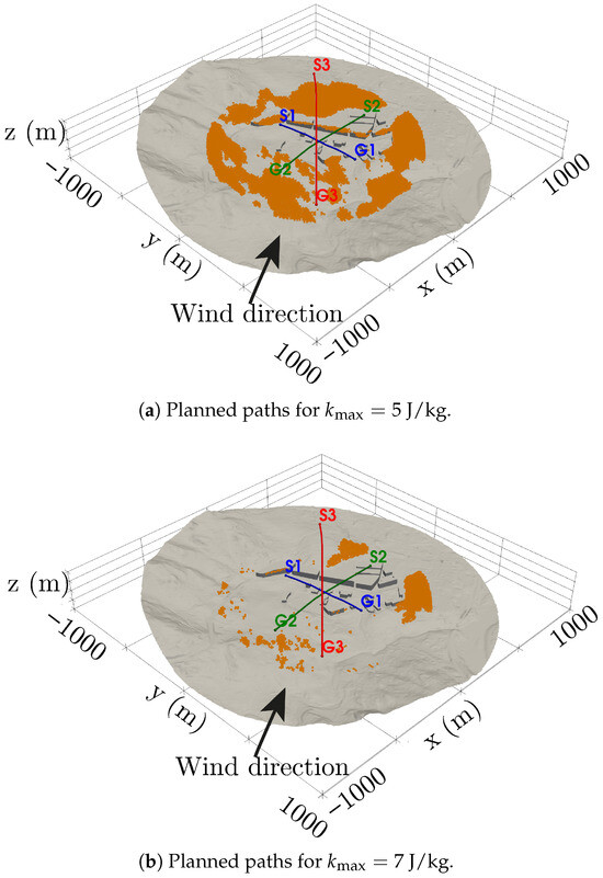
Figure 15.
Computed flight paths for the two turbulence kinetic energy configurations. Orange areas indicate flight restrictions where the turbulence kinetic energy (k) exceeds the defined threshold.
Most turbulence-restricted areas occur in low-altitude zones within the wake of buildings. These areas are more extensive for J/kg, as the stricter threshold limits available flight space. This extensive low-altitude restriction could complicate Urban Air Mobility (UAM) operations.
Table 4 summarises the path lengths for the three trajectories. Since turbulence constraints did not impose any limitations, all path lengths are identical for both values. For Trajectory 1, the total length matches the shortest possible distance, as no obstacles were encountered. The proposed k-NANN approach provides a wide range of movement directions, allowing the aircraft to choose the optimal direction along each edge and avoid the typical zigzag oscillations observed in grid-based planners. Trajectories 2 and 3 are slightly longer than the shortest possible distance, with increases of approximately 2% and 4%, respectively.
4. Conclusions
This study introduces a flexible 3D modelling methodology for developing microweather systems for UAV urban operations. The approach automatically generates OpenFOAM-compatible meshes, incorporating terrain elevation, building geometry, and vegetation. The tool also enables geometry modification and simplification, improving simulation convergence and allowing model complexity to be adjusted according to available computational resources.
As a practical application, a case study was conducted in Ourense (Spain) to analyse the impact of wind on UAV flight conditions. The CFD model was coupled with WRF forecasts to generate high-resolution wind predictions for the area, which were subsequently integrated into a trajectory calculation framework. An uncertainty analysis was performed considering errors in the boundary conditions, and the model was validated against experimental wind measurements. Simulation results showed good agreement with the experimental data despite uncertainties and the use of a RANS model, with relatively small errors: 0.68 m/s for wind velocity, 9.5° for wind direction, and 0.17 J/kg for turbulent kinetic energy.
Future work will assess the impact of turbulence on UAV performance using state-of-the-art simulators incorporating non-stationary aerodynamic models. In addition, the proposed concept will be further validated through experimental campaigns conducted in more urban settings including multi-height measurements and by employing LES models in smaller domains.
Author Contributions
Conceptualization, E.A., G.V.-P., P.D.-E., E.M., F.V.-L., G.F.-C., and H.G.-J.; methodology, E.A., G.V.-P., P.D.-E., E.M., F.V.-L., G.F.-C., and H.G.-J.; software, E.A., G.V.-P., and P.D.-E.; validation, E.M., F.V.-L., and H.G.-J.; formal analysis, E.M., F.V.-L., and H.G.-J.; investigation, E.A., G.V.-P., P.D.-E., E.M., and G.F.-C.; resources, H.G.-J. and F.V.-L.; data curation, E.A., G.V.-P. and P.D.-E.; writing—original draft preparation, E.A. and G.V.-P.; writing—review and editing, E.M., F.V.-L., G.F.-C., and H.G.-J.; visualization, E.A. and G.V.-P.; supervision, E.M., F.V.-L., and H.G.-J.; project administration, E.M. and H.G.-J.; funding acquisition, E.M. and H.G.-J. All authors have read and agreed to the published version of the manuscript.
Funding
This work was funded by the European Union: Horizon Europe, Agencia Estatal de Investigación, Ministerio de Ciencia, Innovación y Universidades, and Xunta de Galicia through the following grants: SARIL A302, STORCITO 101182153, RADIANCE 101235536, PID2021-125060OB-I00 A202, CPP2022-009679 A308, FPU21/01176, FEADER2024/052B A406, Ciencias Mariñas-MRR C286, CO-0091-2024.
Data Availability Statement
Data will be made available on request.
Conflicts of Interest
The authors declare no conflicts of interest.
References
- González-Jorge, H.; Martínez-Sánchez, J.; Bueno, M.; Arias, P. Unmanned Aerial Systems for Civil Applications: A Review. Drones 2017, 1, 2. [Google Scholar] [CrossRef]
- Mohsan, S.A.H.; Khan, M.A.; Noor, F.; Ullah, I.; Alsharif, M.H. Towards the Unmanned Aerial Vehicles (UAVs): A Comprehensive Review. Drones 2022, 6, 147. [Google Scholar] [CrossRef]
- Cheng, N.; Wu, S.; Wang, X.; Yin, Z.; Li, C.; Chen, W.; Chen, F. AI for UAV-Assisted IoT Applications: A Comprehensive Review. IEEE Internet Things J. 2023, 10, 14438–14461. [Google Scholar] [CrossRef]
- Zhang, H.; Wang, F.; Feng, D.; Du, S.; Zhong, G.; Deng, C.; Zhou, J. A Logistics UAV Parcel-Receiving Station and Public Air-Route Planning Method Based on Bi-Layer Optimization. Appl. Sci. 2023, 13, 1842. [Google Scholar] [CrossRef]
- Aurambout, J.P.; Gkoumas, K.; Ciuffo, B. Last mile delivery by drones: An estimation of viable market potential and access to citizens across European cities. Eur. Transp. Res. Rev. 2019, 11, 30. [Google Scholar] [CrossRef]
- She, R.; Ouyang, Y. Efficiency of UAV-based last-mile delivery under congestion in low-altitude air. Transp. Res. Part C Emerg. Technol. 2021, 122, 102878. [Google Scholar] [CrossRef]
- Barrado, C.; Boyero, M.; Brucculeri, L.; Ferrara, G.; Hately, A.; Hullah, P.; Martin-Marrero, D.; Pastor, E.; Rushton, A.P.; Volkert, A. U-Space Concept of Operations: A Key Enabler for Opening Airspace to Emerging Low-Altitude Operations. Aerospace 2020, 7, 24. [Google Scholar] [CrossRef]
- Tepylo, N.; Straubinger, A.; Laliberte, J. Public perception of advanced aviation technologies: A review and roadmap to acceptance. Prog. Aerosp. Sci. 2023, 138, 100899. [Google Scholar] [CrossRef]
- Reiche, C.; Cohen, A.P.; Fernando, C. An Initial Assessment of the Potential Weather Barriers of Urban Air Mobility. IEEE Trans. Intell. Transp. Syst. 2021, 22, 6018–6027. [Google Scholar] [CrossRef]
- Mohamed, A.; Marino, M.; Watkins, S.; Jaworski, J.; Jones, A. Gusts Encountered by Flying Vehicles in Proximity to Buildings. Drones 2023, 7, 22. [Google Scholar] [CrossRef]
- Gendron, É.; Leclerc, M.A.; Hovington, S.; Perron, É.; Rancourt, D.; Lussier-Desbiens, A.; Hamelin, P.; Girard, A. Assessing wind impact on semi-autonomous drone landings for in-contact power-line inspection. Drone Syst. Appl. 2024, 12, 1–16. [Google Scholar] [CrossRef]
- Geronel, R.S.; Botez, R.M.; Bueno, D.D. Dynamic responses due to the Dryden gust of an autonomous quadrotor UAV carrying a payload. Aeronaut. J. 2023, 127, 116–138. [Google Scholar] [CrossRef]
- Mendez, A.P.; Whidborne, J.F.; Chen, L. Wind Preview-Based Model Predictive Control of Multi-Rotor UAVs Using LiDAR. Sensors 2023, 23, 3711. [Google Scholar] [CrossRef]
- Simon, N.; Ren, A.Z.; Piqué, A.; Snyder, D.; Barretto, D.; Hultmark, M.; Majumdar, A. FlowDrone: Wind Estimation and Gust Rejection on UAVs Using Fast-Response Hot-Wire Flow Sensors. In Proceedings of the 2023 IEEE International Conference on Robotics and Automation (ICRA), London, UK, 29 May–2 June 2023; pp. 5393–5399. [Google Scholar] [CrossRef]
- Semenov, S.; Jian, Y.; Jiang, H.; Chernykh, O.; Binkovska, A. Mathematical model of intelligent UAV flight path planning. Adv. Inf. Syst. 2025, 9, 49–61. [Google Scholar] [CrossRef]
- Steiner, M. Urban Air Mobility: Opportunities for the Weather Community. Bull. Am. Meteorol. Soc. 2019, 100, 2131–2133. [Google Scholar] [CrossRef]
- Adkins, K.A.; Becker, W.; Ayyalasomayajula, S.; Lavenstein, S.; Vlachou, K.; Miller, D.; Compere, M.; Muthu Krishnan, A.; Macchiarella, N. Hyper-Local Weather Predictions with the Enhanced General Urban Area Microclimate Predictions Tool. Drones 2023, 7, 428. [Google Scholar] [CrossRef]
- Zhang, S.; Kwok, K.C.; Liu, H.; Jiang, Y.; Dong, K.; Wang, B. A CFD study of wind assessment in urban topology with complex wind flow. Sustain. Cities Soc. 2021, 71, 103006. [Google Scholar] [CrossRef]
- Qi, Y.; Ishihara, T. Numerical study of turbulent flow fields around of a row of trees and an isolated building by using modified k-ε model and LES model. J. Wind Eng. Ind. Aerodyn. 2018, 177, 293–305. [Google Scholar] [CrossRef]
- Ampatzidis, P.; Cintolesi, C.; Petronio, A.; Di Sabatino, S.; Kershaw, T. Evaporating waterbody effects in a simplified urban neighbourhood: A RANS analysis. J. Wind Eng. Ind. Aerodyn. 2022, 227, 105078. [Google Scholar] [CrossRef]
- Nithya, D.S.; Quaranta, G.; Muscarello, V.; Liang, M. Review of Wind Flow Modelling in Urban Environments to Support the Development of Urban Air Mobility. Drones 2024, 8, 147. [Google Scholar] [CrossRef]
- Blocken, B. LES over RANS in building simulation for outdoor and indoor applications: A foregone conclusion? Build. Simul. 2018, 11, 821–870. [Google Scholar] [CrossRef]
- Paden, I.; García-Sánchez, C.; Ledoux, H. Towards automatic reconstruction of 3D city models tailored for urban flow simulations. Front. Built Environ. 2022, 8, 899332. [Google Scholar] [CrossRef]
- Deininger, M.E.; von der Grün, M.; Piepereit, R.; Schneider, S.; Santhanavanich, T.; Coors, V.; Voß, U. A Continuous, Semi-Automated Workflow: From 3D City Models with Geometric Optimization and CFD Simulations to Visualization of Wind in an Urban Environment. ISPRS Int. J. Geo-Inf. 2020, 9, 657. [Google Scholar] [CrossRef]
- Slotnick, J.P.; Khodadoust, A.; Alonso, J.J.; Darmofal, D.L.; Gropp, W.; Lurie, E.A.; Mavriplis, D.J. CFD Vision 2030 Study: A Path to Revolutionary Computational Aerosciences; NASA Center for AeroSpace Information: Hanover, MD, USA, 2014. [Google Scholar]
- Biljecki, F.; Ledoux, H.; Du, X.; Stoter, J.; Soon, K.H.; Khoo, V.H.S. The most common geometric and semantic errors in CityGML datasets. ISPRS Ann. Photogramm. Remote Sens. Spat. Inf. Sci. 2016, IV-2/W1, 13–22. [Google Scholar] [CrossRef]
- Lin, L.; Liu, Y.; Hu, Y.; Yan, X.; Xie, K.; Huang, H. Capturing, Reconstructing, and Simulating: The UrbanScene3D Dataset. arXiv 2022, arXiv:2107.04286. [Google Scholar] [CrossRef]
- Zhao, J.; Stoter, J.; Ledoux, H. A Framework for the Automatic Geometric Repair of CityGML Models. In Cartography from Pole to Pole: Selected Contributions to the XXVIth International Conference of the ICA, Dresden 2013; Springer: Berlin/Heidelberg, Germany, 2014; Chapter 14; pp. 187–202. [Google Scholar] [CrossRef]
- Mirzaei, P.A. CFD modeling of micro and urban climates: Problems to be solved in the new decade. Sustain. Cities Soc. 2021, 69, 102839. [Google Scholar] [CrossRef]
- Blocken, B. Computational Fluid Dynamics for urban physics: Importance, scales, possibilities, limitations and ten tips and tricks towards accurate and reliable simulations. Build. Environ. 2015, 91, 219–245. [Google Scholar] [CrossRef]
- Boikos, C.; Siamidis, P.; Oppo, S.; Armengaud, A.; Tsegas, G.; Mellqvist, J.; Conde, V.; Ntziachristos, L. Validating CFD modelling of ship plume dispersion in an urban environment with pollutant concentration measurements. Atmos. Environ. 2024, 319, 120261. [Google Scholar] [CrossRef]
- Badach, J.; Wojnowski, W.; Gebicki, J. Spatial aspects of urban air quality management: Estimating the impact of micro-scale urban form on pollution dispersion. Comput. Environ. Urban Syst. 2023, 99, 101890. [Google Scholar] [CrossRef]
- Brozovsky, J.; Simonsen, A.; Gaitani, N. Validation of a CFD model for the evaluation of urban microclimate at high latitudes: A case study in Trondheim, Norway. Build. Environ. 2021, 205, 108175. [Google Scholar] [CrossRef]
- Blocken, B.; van der Hout, A.; Dekker, J.; Weiler, O. CFD simulation of wind flow over natural complex terrain: Case study with validation by field measurements for Ria de Ferrol, Galicia, Spain. J. Wind Eng. Ind. Aerodyn. 2015, 147, 43–57. [Google Scholar] [CrossRef]
- Ledoux, H.; Biljecki, F.; Dukai, B.; Kumar, K.; Peters, R.; Stoter, J.; Commandeur, T. 3dfier: Automatic reconstruction of 3D city models. J. Open Source Softw. 2021, 6, 2866. [Google Scholar] [CrossRef]
- Mahgoub, A.O.; Ghani, S. Numerical and experimental investigation of utilizing the porous media model for windbreaks CFD simulation. Sustain. Cities Soc. 2021, 65, 102648. [Google Scholar] [CrossRef]
- Li, R.; Niu, J.; Zhao, Y.; Wang, L.L.; Shi, X.; Gao, N. Wind tunnel experiments on the aerodynamic effects of a single potted tree: Hot-wire anemometry and PIV measurements. Urban Clim. 2025, 62, 102520. [Google Scholar] [CrossRef]
- Pardo-del Viejo, L.; Fernández-Rodríguez, S. CFD with LIDAR applied to buildings and vegetation for environmental construction. Autom. Constr. 2024, 167, 105710. [Google Scholar] [CrossRef]
- Huo, H.; Chen, F. Study of effects of different vegetation model parameter settings on quantitative CFD simulation of urban spatial air temperature and wind-field. Int. J. Remote Sens. 2023, 45, 7234–7247. [Google Scholar] [CrossRef]
- Aldao, E.; Fontenla-Carrera, G.; Veiga-López, F.; González-Jorge, H.; Morais, M.J.; Matos, J.C. Evaluating the Influence of Wind on UAV Path Planning for Bridge Inspections. In Proceedings of the 2025 International Conference on Unmanned Aircraft Systems (ICUAS), Charlotte, NC, USA, 14–17 May 2025; pp. 236–242. [Google Scholar] [CrossRef]
- Instituto Geográfico Nacional. Centro de Descargas, 2024. Available online: https://centrodedescargas.cnig.es/CentroDescargas/home (accessed on 4 October 2024).
- An, K.; Wong, S.M.; Fung, J.C.H.; Ng, E. Revisit of prevailing practice guidelines and investigation of topographical treatment techniques in CFD-Based air ventilation assessments. Build. Environ. 2020, 169, 106580. [Google Scholar] [CrossRef]
- Biljecki, F.; Ledoux, H.; Stoter, J. An improved LOD specification for 3D building models. Comput. Environ. Urban Syst. 2016, 59, 25–37. [Google Scholar] [CrossRef]
- Silva, J.; Ribeiro, C.; Guedes, R.; Rua, M.C.; Ulrich, F. Roughness length classification of Corine Land Cover classes. In Proceedings of the EWEC 2007, Milan, Italy, 7–10 May 2007. [Google Scholar]
- MeteoGalicia. Modelos Meteorológicos Deterministas, 2024. Available online: https://www.meteogalicia.gal/web/observacion/meteovisor (accessed on 4 October 2024).
- SIMSCALE. Advanced Modelling PWC, 2024. Available online: https://www.simscale.com/docs/analysis-types/pedestrian-wind-comfort-analysis/advanced-modelling/ (accessed on 4 October 2024).
- Iio, A.; Ito, A. A Global Database of Field-Observed Leaf Area Index in Woody Plant Species, 1932–2011; ORNL Distributed Active Archive Center: Oak Ridge, TN, USA, 2014. [Google Scholar] [CrossRef]
- Bekkers, C.C.; Angelou, N.; Dellwik, E. Drag coefficient and frontal area of a solitary mature tree. J. Wind Eng. Ind. Aerodyn. 2022, 220, 104854. [Google Scholar] [CrossRef]
- Aldao, E.; Veiga-López, F.; Chanel, C.P.; Watanabe, Y.; González-Jorge, H. Dynamic UAV trajectory optimisation for parcel delivery with integrated third-party risk mitigation. Reliab. Eng. Syst. Saf. 2025, 262, 111178. [Google Scholar] [CrossRef]
- GU, R.; ZHAO, Y.; REN, X. Integrating wind field analysis in UAV path planning: Enhancing safety and energy efficiency for urban logistics. Chin. J. Aeronaut. 2025, 103605. [Google Scholar] [CrossRef]
- Gao, M.; Hugenholtz, C.H.; Fox, T.A.; Kucharczyk, M.; Barchyn, T.E.; Nesbit, P.R. Weather constraints on global drone flyability. Sci. Rep. 2021, 11, 12092. [Google Scholar] [CrossRef] [PubMed]


Disclaimer/Publisher’s Note: The statements, opinions and data contained in all publications are solely those of the individual author(s) and contributor(s) and not of MDPI and/or the editor(s). MDPI and/or the editor(s) disclaim responsibility for any injury to people or property resulting from any ideas, methods, instructions or products referred to in the content. |
© 2025 by the authors. Licensee MDPI, Basel, Switzerland. This article is an open access article distributed under the terms and conditions of the Creative Commons Attribution (CC BY) license (https://creativecommons.org/licenses/by/4.0/).