Tracking Fin Whale Morphology with Drone Photogrammetry: Growth Tendencies, Developmental Changes, and Sexual Dimorphism

Abstract

Morphological changes during body development measurements are crucial in understanding growth rates, allometric relationships, and sexual dimorphism. Recent advances in drone technology provide a new perspective enabling an indirect, non-invasive morphological assessment of free-ranging cetaceans. In this study, 10 body parameters were measured and examined with drone-based aerial photogrammetry across 82 individual fin whales (Balaenoptera physalus) along the Catalan coast of the Northwestern Mediterranean Sea, between 2021 and 2023. The growth pattern of each body parameter relative to the total length was determined as negative allometry. The developmental changes depicted that the head region at first decreases proportionally until the animal reaches approximately 14 m in length. Then, it remains constant until 18 m, subsequently followed by a relative increase. The difference in the growth rates among the sexes leads to a proportional shift between females and males approximately between 15 and 17 m in length. Overall, males exhibit a more rapid body elongation, along with moderate development of the other body parameters, while females display the contrary. The morphological parameters reveal insights into the population status dynamics and provide information on the reproductive status. These parameters are critical for the proper conservation and management of the local population of the species.

1. Introduction

Fin whales (Balaenoptera physalus) are the second largest species of baleen whales, with slender bodies reaching approximately 18 to 27 m in length [1,2]. The species exhibits pronounced sexual dimorphism, with females attaining larger body sizes than males by approximately 5–10% of the total length [2]. Generally, fin whales in the Northern Hemisphere tend to grow smaller than those in the Southern Hemisphere [3].

Fin whales are migratory species, following an annual movement pattern between feeding and breeding grounds [4]. Moreover, they are the only baleen whale species present year-round in the Mediterranean Sea [4,5,6], where two distinct populations have been identified: the North East North Atlantic (NENA) population and the Mediterranean subpopulation [7,8,9,10]. Fin whales are frequently sighted near the Catalan coast of Spain in the Balearic Basin between March and May [6,8,11,12,13]. This area has been described as the foraging ground [8,11,12,14].

Growth is a critical factor and a reliable indicator of age, sexual maturity, longevity, fitness, and population status [15,16,17]. Furthermore, it provides information on body development, during which characteristic proportional changes occur [17,18]. Mysticetes, including fin whales, exhibit some of the most rapid growth rates and body development, allowing them to enhance survival rates and maximize fitness [19,20].

Studying fin whales presents significant challenges due to their fast-moving, free-ranging, pelagic, and elusive nature [21,22,23,24]. Traditionally, morphological analyses of such large cetaceans were limited to direct measures of stranded animals or specimens obtained from whaling activities [1,18,25]. In recent years, unmanned aerial vehicles (UAVs), commonly known as drones, created a new, safe, and non-invasive method for collecting large amounts of aerial footage of targeted species [26,27]. Aerial photogrammetry enables precise morphometric measurements by analyzing vertical images based on specific parameters of the UAV’s sensors. These pixel-based measurements are then scaled to real-world units (meters) using a calibration object of known size, ensuring the most accurate size estimate of the whales [25,28]. This indirect measurement approach enables the assessment of various body parameters [29]. Additionally, both temporary and permanent changes in the body morphology can be followed over time, providing valuable insight into growth patterns, allometric relationships [29], and sex-based variation [18]. These morphological attributes are essential for monitoring the local population to assess the population status and health [28,30]. Moreover, investigating the variation in the body parameters helps identify sexual differences in proportions and growth tendencies [31].

The aim of this study was to implement drone photogrammetry as a method for monitoring and analyzing growth rates, proportional changes during body development, and the overall morphology of fin whales (Balaenoptera physalus). Furthermore, the project sought to investigate variations in these morphological attributes between sexes. The project was conducted between 2021 and 2023 in the course of three consecutive feeding seasons, occurring from March to May. During this time period, fin whales migrate to the Balearic Basin in the Northwestern Mediterranean Sea, where they are found in close proximity to the Catalan coast of Spain.

2. Materials and Methods

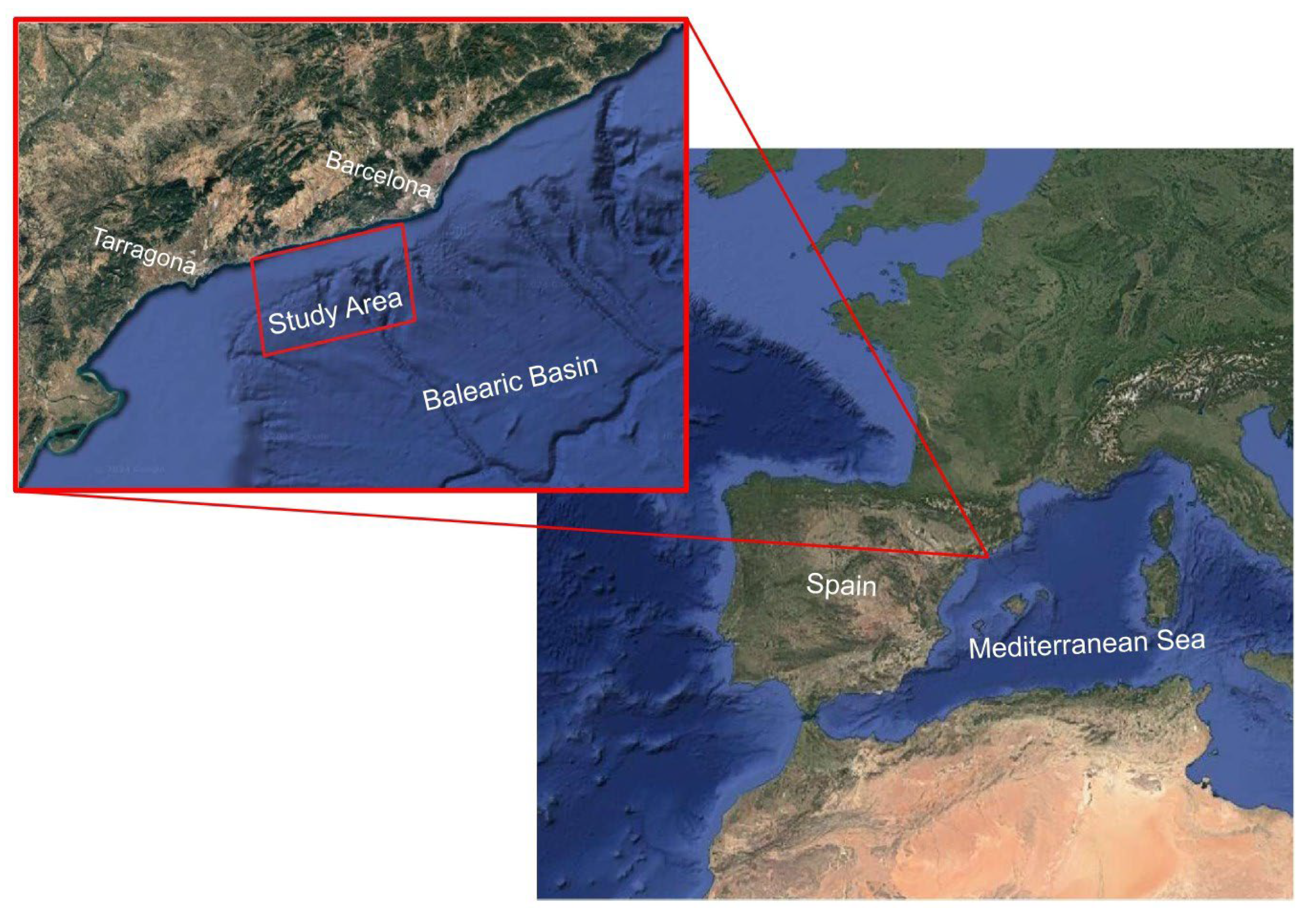
2.1. Study Area

This research was conducted in a geographically distinct foraging ground in the Northwestern Mediterranean Sea, along the Spanish coastline, approximately between Barcelona and Tarragona within the Balearic Basin [11]. The area covers approximately 1.944 km² extending 10 to 15 miles from shore (Figure 1) [8]. It lies between the Ebro and the Llobregat rivers, whose nutrient input influences the primary production of the area [32,33]. Additionally, the Cunit and Foix submarine canyons contribute to prey availability through upwelling processes [8,34].

2.2. Data Collection

Data collection took place from March to May over three foraging seasons (2021–2023), during which fin whales migrate to this area to feed [8,11]. Daily surveys were conducted in random transects across the study area. Fieldwork was carried out aboard of the research vessel MAKTUB, a 14.15 m long Catana catamaran operated by EDMAKTUB research organization [8]. Aerial footage was collected using a Mavic 2 Pro and a Mavic 3 UAVs (manufacturer: DJI, Shenzen, China). The drone flight procedures, photo-identification process, and subsequent cataloging followed the methodology established by Degollada et al. [11] and was conducted under the regulations [35]. The drone-assisted photogrammetric data collection was performed based on the protocol described by Burnett et al. [20]. To ensure measurement accuracy and provide a reference scale, aerial images of a calibration object of known longitude (4.25 m long kayak) were captured using UAVs, following the calibration method developed by Bierlich et al. [36].

2.3. Morphometric Measurements and Scaling

The drone footage was processed following the approach of Soledade et al. [37]. The goal was to extract at least three images per flight from individual whales to average future measurements and minimize precision errors [38].

Body measurements were conducted following the method described by Torres and Bierlich [28] using the MorphoMetrix program version 1. Nine standard cetacean body proportions were assessed and are depicted in Figure 2 and

Table 1. Standard cetacean body proportion measurements.

Body Measurement	Description	Abbreviation
Total length	From the tip of the rostrum until the notch of the fluke	TL
Fluke spread	Width of the fluke	FS
Snout to blowhole	From the tip of the rostrum until the anterior of the blowhole	SB
Snout to dorsal fin	From the tip of the rostrum until the tip of the dorsal fin	SD
Snout anterior flipper	From the tip of the rostrum until the anterior insertion of the flipper	SAF
Snout posterior flipper	From the tip of the rostrum until the anterior–posterior of the flipper	SPF
Anterior flipper length	From the anterior flipper insertion until the tip of the flipper	AFL
Posterior flipper length	From the posterior flipper insertion until the tip of the flipper	PFL
Eye to eye	Width between the eyes	ETE

[30]. Moreover, the general width was measured at 20 locations, by dividing the body into equal segments along the length. At each section, two outlines were manually marked, and the width measurements were calculated between them [39]. All the above-mentioned parameters were manually designated for the pixel-based measurements [16].

2.4. Body Area Index

The body area index (BAI) is a continuous, scale-invariant, and unitless measure. It is a length normalized surface area index that facilitates the comparison of body size and condition over time [25,37]. BAI was estimated using the parabolic fit in the MorphoMetriX program [28]. The index was calculated between 20% and 60% of the total length based on the width measurements. This region represents the torso of the animal where the energy reserve accumulates [37,39].

2.5. Body Development

Several body proportions were calculated to predict the development of different anatomical regions and to examine their relationship [15,23]. Consequently, the following proportions were created and listed in

Table 2. Comparative whale body proportions.

Body Proportions	Abbreviation
Fluke spread compared to total length	FS:TL
Snout to blowhole compared to total length	SB:TL
Snout to dorsal fin compared to total length	SD:TL
Snout to anterior flipper compared to total length	SAF:TL
Snout to posterior flipper compared to total length	SPF:TL
Eye to eye distance compared to total length	ETE:TL
Anterior flipper length compared to total length	AFL:TL
Posterior flipper length compared to total length	PFL:TL
Eye to eye distance compared to snout to blowhole	ETE:SB
Eye to eye distance compared to snout to dorsal fin	EYE:SD
Eye to eye distance compared to fluke spread	EYE:FS
Anterior flipper length compared to eye to eye distance	AFL:ETE
Anterior flipper length compared to snout to blowhole	AFL:SB
Anterior flipper length compared to snout to dorsal fin	AFL:SD
Anterior flipper length compared to fluke spread	AFL:FS
fluke spread compared to snout to blowhole	FS:SB
fluke spread compared to snout to dorsal fin	FS:SD

.

2.6. Photo-Identification and Life-History Traits

Aerial photo-identification technique based on drone imaging described by Degollada et al. [11] was applied to still images obtained from the aerial footage to identify individual animals.

Life history traits, including sex, were determined through biopsies collected during the field surveys [11], which were subsequently processed and analyzed at the Institute of Evolutionary Life Sciences, University of Groningen, The Netherlands.

2.7. Mitigation of Uncertainties

Data obtained from drone-assisted aerial photogrammetry has several uncertainties, including errors related to the animal’s body position, lens distortion, altitude accuracy, and masking environmental conditions [40,41]. Furthermore, precision errors may arise from the manually designated morphometric measurements [38,41]. For both drones, the absolute error was calculated using of 20 vertical aerial images of calibration objects with a known length, captured between 10 and 100 m [27,28,37,42]. The average absolute error was then derived from the 20 outputs followed by the determination average photogrammetric error [30]. To further enhance accuracy, measurements of fin whales identified as the same individual, evaluated from the same aerial footage recorded on the same day were averaged. This approach minimized precision error associated with the manual designation of the body length measurements [27,37,38,41].

2.8. Statistical Analysis

Statistical analyses were performed in R (version 4.0.3) and RStudio (Version: 2023.03.1+446 (R Core Team, 2023)), using the following packages: cowplot, dplyr, factoextra, flextable, FSA, gapminder, geomextpath, GGally, ggforce, ggplot2, ggpubr, ggstatsplot, hrbrthemes, lubridate, pdfetch, Rcmdr, readxl, remotes, sjlabelled, sjmisc, sjPlot, tibble, tidyr, tdyvers, vctrs, versions, and xts [43,44,45,46,47,48,49,50,51,52,53,54,55,56,57,58,59,60,61,62,63,64,65,66,67,68,69].

Body measurements of individual whales, obtained on the same day were averaged prior to the analysis.

Afterward, the variables were tested for normal distribution using the Kolmogorov–Smirnov test of normality (p-value < 0.05), and Levene’s test was applied to test homogeneity (p-value < 0.05). As the normality and homoscedasticity of the variables could not be accepted, and the parameters followed a log-normal distribution, a logarithmic transformation was performed.

Individual whales with missing values were omitted from further analysis to ensure accuracy and consistency in the investigations [60].

2.8.1. Body Size

Firstly, the numerical variables were summarized to obtain general information and sex-based differences upon the body length.

To investigate the correlation between the logarithmically transformed body parameters (TL, SB, SD, SAF, SPF, AFL, PFL, FS, and ETE) a correlation matrix was created. The growing rates of length and width change over time [70], therefore a k-mean cluster method was applied to create size subgroups using the TL and ETE parameters. Consequently, three distinctive clusters were defined, and the whales were assigned into the following size groups: small, animals under 15 m; medium, between 15 and 18 m; and large, whales above 18 m.

2.8.2. Allometric Growth

To identify the allometric growth relationship, eight body measurements were regressed against the TL. Growth trends were determined using the following equation:

Y = aXb,

(1)

where Y = TL (m), X = body parameter (m), a = intercept, and b = allometric coefficient.

2.8.3. Developmental Changes

Growth ratios and developmental changes were analyzed on the previously described body proportion (Section 2.5). These proportions were created and added to the dataset. Changes were examined by plotting each body proportion relative to the total length. Furthermore, these parameters were also compared to the eye to eye width (ETE) and to the snout to blowhole (SB) and therefore, plotted against them. To help visualize the variation a LOWESS (locally weighted scatterplot smoothing) was added to the plots. Which is a nonparametric approach to fit a smooth curve to the data [71].

2.8.4. Sexual Dimorphism

Sexual dimorphism was investigated by Spearman’s rank correlation coefficient, which tests the relationship between the individual mean of each measured body parameters (TL~ETE, TL~FS, TL~SB, TL~SD, TL~SAF, TL~SPF, TL~AFL, TL~PFL, ETE~FS, ETE~SB, ETE~SD, ETE~AFL, ETE~SAF, FS~SB, FS~SD, and FS~AFL) per sexes.

Moreover, multivariate ANOVA analysis was performed to further investigate sexual dimorphism, where nine morphological body measures were examined as dependent variables [24].

Furthermore, linear regression models were generated to investigate the relationships between the nine previously logarithmically transformed body parameters and the total length of the body. All these models were made according to the assumptions of linear models beforehand; normality and homogeneity of residuals and related diagnostic plots were performed. The models which attained an adjusted R-square close to 1, p-value < 0.05, had significant variables (significance < 0.01), and had residuals that met the assumptions (homogeneity and normality) were accepted. Parameters obtaining significant results were further analyzed to determine if sex is an influencing factor. When significant influences (significance < 0.01) of the tested factors (sex) were observed, separated Linear Models were created for each subgroup (female, male) to identify the precise differences between them. Body parameters obtaining significant results (significance < 0.01) were plotted together, showcasing the separated models per group, scaled to the original dataset to visualize the disparity between sexes.

The non-parametric Kruskal–Wallis test (p-value < 0.05) was applied to test for potential significant differences existing between the BAI measurements among the sexes and size groups.

3. Results

A total of 366 sequences of aerial footage (2021: 193, 2022: 109, 2023: 67) were analyzed, resulting in 1099 captured and measured still images (2021: 426, 2022: 256, 2023: 415), depicting 82 individual fin whales. During the three examined seasons, 17 females, 13 males, and 52 individuals with unknown sex were analyzed.

3.1. Body Size

Fin whales along the Catalan coast during the time period of 2021–2023 had an average body length of 16.38 m (Std = 2.49). The smallest recorded individual was a 9.49 m long calf, while the largest, an animal of unknown sex, measured 24.45 m. The average body length of 17.63 (Std = 1.99) meters for females and 15.68 m (Std = 2.65) for males, with an average difference of 1.95 m.

The categorization of animals by size resulted in 21 animals in the small size group (under 15 m), 111 animals in the medium size group (between 15 and 18 m), and 20 animals in the large size group (over 18 m).

The gender distribution among size groups (Figure 3) indicates that a significant proportion of the large size group (female = 9, male = 5, unknown = 13) consists of female individuals, similar to the medium size group (female = 10, male = 6, unknown = 31). In contrast, the small size group (female = 2, male = 8, unknown = 21) is male dominated. However, individuals with unknow sex comprise the largest proportion across all groups.

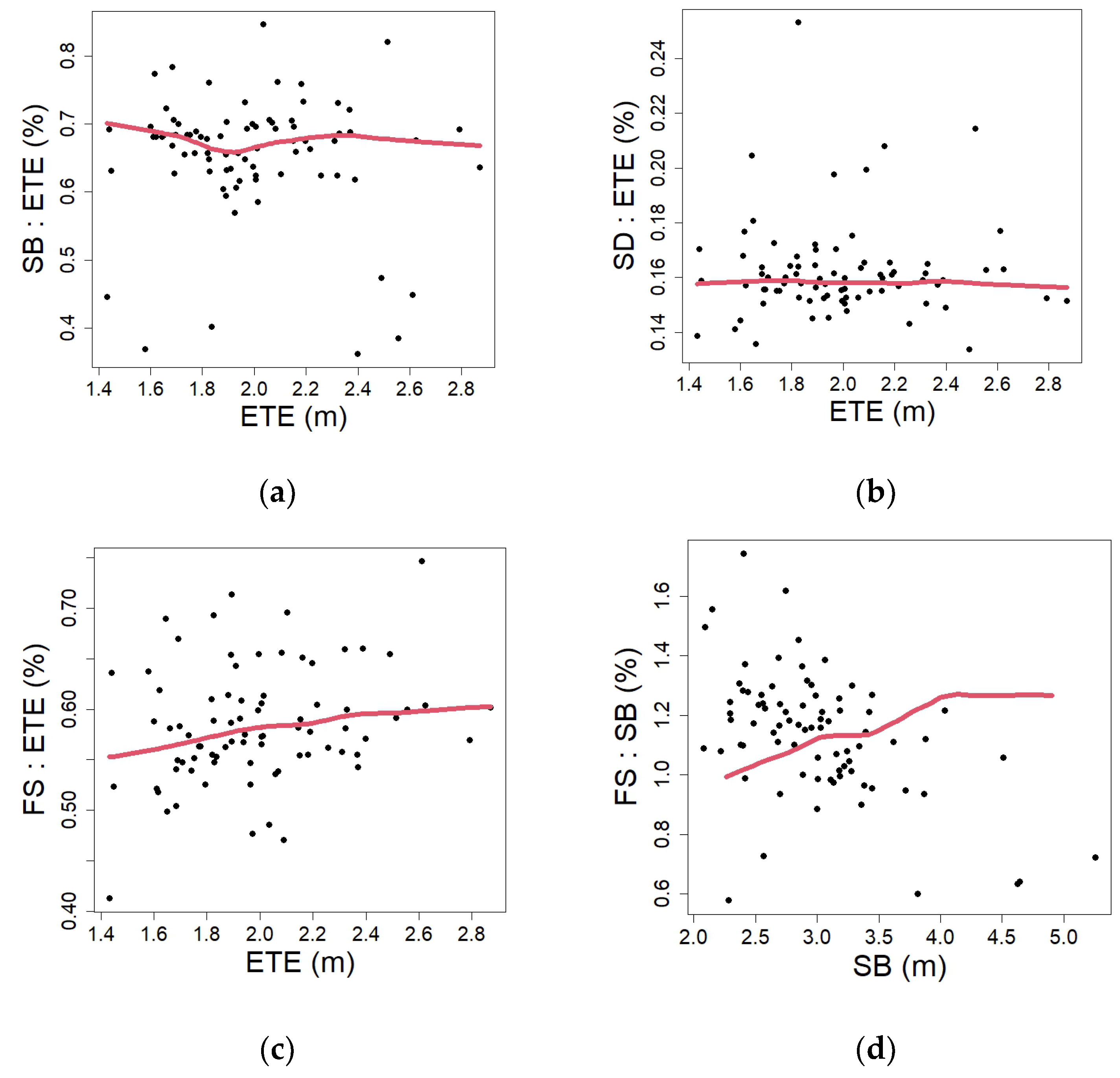
3.2. Allometric Growth

The allometric relationship and growth patterns of various body parameters were investigated, with positive allometry identified when the coefficient exceeded 1 and negative allometry when below 1 [15,24].

The results in

Table 3. Allometric growth relationships of eight body measurements in relation to TL. Where R² = correlation coefficient, SER = standard deviation of the residuals.

Abbreviation	N	R2	Intercept	Allometric Coefficient	Relative Growth Pattern	SER (%)
ETE	106	0.800	0.39	−0.792	Negative	0.6
FS	107	0.698	0.38	−0.527	Negative	0.2
SB	100	0.514	0.47	−0.833	Negative	0.1
SD	90	0.844	0.48	−0.238	Negative	0.07
AFL	102	0.730	0.37	−0.764	Negative	0.2
PFL	100	0.677	0.38	−0.949	Negative	0.4
SAF	102	0.420	0.41	−0.476	Negative	0.8
SPF	102	0.806	0.44	−0.482	Negative	0.8

indicate negative allometry (allometric coefficient < 0) for all morphometric parameters at a 95% confidence interval. The highest allometric coefficient was obtained between the SD~TL, followed closely by SAF~TL and SPF~TL. While the lowest coefficient was found at the PFL~TL.

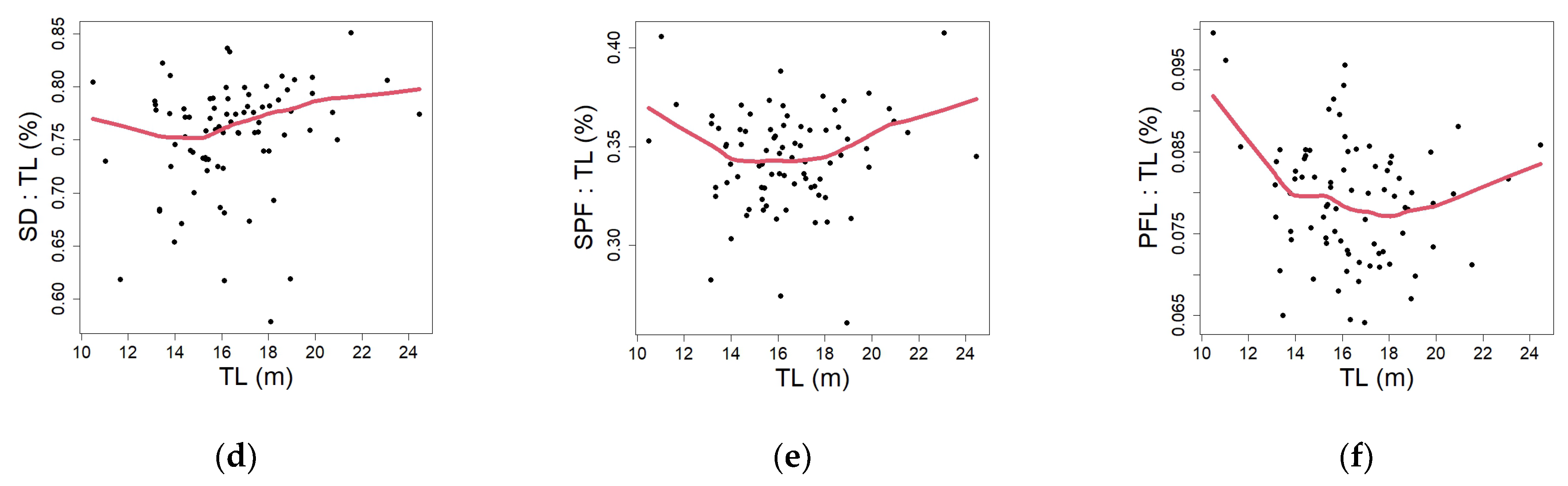
3.3. Developmental Changes

The LOWESS smoothing curves in Figure 4 illustrate the changes in six standard whale body proportions (ETE, FS, SB, SD, SPF, and PFL) relative to the body length.

Graphs (a) and (b) exhibited comparable slopes, with both curves initially declining until approximately 14–15 m. Between 18 and 20 m, the trends stabilize before beginning to decline again. Similarly, graphs (c) and (e) displayed analogous patterns, showing an initial decline followed by stabilization; however, after 18–19 m, they gradually increased. This indicates that ETE-FS and SB-SPF undergo similar proportional changes relative to the body length. Graph (d) showcases the snout to blowhole (SD), which body proportion initially decreases, similar to the previous trends. Withal, this region exhibited the most continuous increases in relative size. Finally, graph (f), which represents the posterior flipper length and was the only parameter exhibiting a continuous and gradual decline. Overall, each graph illustrates that all parameters vary in proportion as the animals attain greater body length.

The variation in the proportions based on the LOWESS curve in graph (a) of Figure 5 depicts a general, but minor decrease in the area of the SB relative to the ETE with a slight increase between 1.9 and 2.3 m in the width of the ETE. Graph (b) represents the SD, which follows a very steady trend with only a minor decline. The final two graphs illustrate the FS, with graph (c) depicting its relation to ETE and graph (d) comparing it to the SB. Both graphs exhibit increasing slopes; however, while graph (c) shows a gradual increase, graph (d) displays a more fluctuating pattern.

3.4. Sexual Dimorphism

The correlation between the measured body parameters for each sex was tested with Spearman’s rank correlation coefficient analysis. The strength of the correlation was categorized as: very weak < 0.19, 0.2 < weak > 0.39, 0.4 < moderate > 0.59, 0.6 < strong > 0.79, and 0.8 < very strong > 1 [72]. All tests obtained a p-value below 0.005. Females exhibited a very strong correlation between anatomical regions, including TL~ETE, TL~SB, TL~SD, TL~SAF, and TL~SPF. And a strong correlation between the FS, AFL, and PFL relative to the total length. Meanwhile, males displayed only strong correlations. For proportions relative to the eye to eye distance females obtained a very strong correlation in ETE~SB, ETE~SD, and ETE~SAF, while the remaining parameters had a strong correlation. In males, only ETE~FS exhibited a very strong correlation. Lastly, all body parameters compared to the fluke spread showed strong correlation in both sexes.

The multivariate analysis provided insight to differences in body proportions between the sexes (

Table 4. Results of ANOVA analysis (multivariant) assessing sexual dimorphism. Each body parameter obtained 77 DF.

	Female				Male				ANOVA
Abbreviation	Mean (m)	Std	Range (m)	p-Value	Mean (m)	Std	Range (m)	p-Value	F-Value	p-Value
TL	17.63	1.99	13.76–21.51	0.07	15.71	2.26	11.50–20.73	0.45	3.61	0.14
ETE	2.15	0.31	1.70–2.79	0.01	1.90	0.27	1.43–2.39	0.10	3.09	0.05
FS	3.64	0.45	2.89–4.91	0.03	3.25	0.60	2.38–4.20	0.16	2.23	0.11
SB	3.3	0.56	2.44–4.64	0.02	2.94	0.61	2.21–4.62	0.43	3.15	0.04
SD	13.57	2.01	10.66–18.31	0.01	11.72	2.14	10.31–16.09	0.10	3.63	0.03
AFL	1.95	0.26	1.64–2.56	0.04	1.81	0.30	1.46–2.29	0.53	2.83	0.06
PFL	1.38	0.18	1.10–1.84	0.04	1.26	0.22	1.01–1.65	0.40	2.53	0.08
SAF	5.03	0.92	3.34–6.75	0.18	4.49	1.05	1.75–5.56	0.20	1.00	0.37
SPF	6.05	0.94	5.52–7.68	0.07	5.54	1.03	4.76–7.65	0.45	1.94	0.14

). Females exhibited an overall higher value as they reached a larger body size. Furthermore, females showed lower p-values and standard deviation than males across all parameters. Significant differences between sexes were observed in the body parameters of SB, SD, and ETE. The SB was approximately 19% for females and 20% for males. While the snout to dorsal fin (SD) was 76% in females and 74% in males. The remaining general whale body parameters showed no significant variation between the sexes.

The relationship between various body parameters (

Table 5. Results of linear models obtaining significance in sexual dimorphism.

	Sex		Female	Male
	Adjusted R2	Significance	Adjusted R2	Adjusted R2
ETE~TL	0.7942	<0.001	0.8631	0.7579
SD~TL	0.5175	<0.001	0.6107	0.4698
SB~TL	0.8401	0 < x < 0.001	0.8928	0.8525
SD~ETE	0.689	<0.001	0.6894	0.2957
FS~ETE	0.6234	<0.001	0.5649	0.3827

) and their developmental differences by sex is illustrated in Figure 6 based on the results of the linear regression models. In all cases, both sexes obtained a positive increasing tendency; however, females generally had a steeper upward trajectory, except for FS relative to ETE, in graph (e). Graph (a) showcases the relationship between ETE (y axis) and TL (x axis). The two slopes intersect near the vicinity of 17 m, and females surpass males in ETE distance. Graph (b) represents SD (y axis) in relation to TL (x axis). The ratio of these variables alternates between sexes at approximately 15 m in length. Above this length, females have larger snout to dorsal fin distance relative to their total size, than males. Graph (c) illustrates the relationship between SB (y axis) and TL (x axis). The crossover point, where females surpass males, occurs further on, when the animals reach 18 m TL. Graph (d) depicts the relationship between the SB (y axis) and ETE (x axis). The slopes of the two sexes cross roughly 2.15 m (ETE), after which the two variables diverge. Finally, graph (e) presents the relationship between FS (y axis) and ETE (x axis). The disparity between sexes initiates in the close vicinity of the ETE width of 2.2 m. Below this threshold, females attain wider FS, but beyond this point males overtake the females, developing considerably wider flukes.

The remaining general whale body proportions (SAF, SPF, AFL, and PFL) showed no significant difference between males and females.

There is a clear difference in BAI between the sexes. Figure 7 depicts the mean of the BAI for each size group based on sex. Females (n = 17) obtained a significant, steady increase. Small individuals (n = 1) had the lowest BAI, followed by medium sized animals (n = 13), while the large individuals (n = 3) had the highest BAI. In contrast, males (n = 13) exhibited the opposite tendency. Small (n = 4) animals attained the highest BAI, while those in the large group (n = 1) had the lowest. The decline between the small and medium (n = 8) groups was substantial, whereas the decrease between the medium and large group was more gradual. However, the varying sample size across groups may have influenced the results. Due to this limited sample size, these findings are not fully representative of the population.

The Kruskal–Wallis test showed no statistically significant variation in mean BAI between the sexes (p-value: 0.063).

3.5. Uncertanties

The averaged absolute error was 0.36 for UAV Mavic Pro 2, and 0.41 for Mavic 3. Furthermore, the average photogrammetric error was 0.025 (2.5%) for Mavic 2 Pro and 0.098 (9.8%) for the Mavic 3. These errors lead to a minor overestimation of size ranging from approximately 10 to 40 cm.

Moreover, repeated measurements of the same individual, from the same flight footage showed a mean body length estimation error between 0.46% and 6.82%.

4. Discussion

During this study the aerial perspective of the UAV permitted to record vertical images of the encountered fin whales, facilitating the quantification of the body size and other body parameters. This demonstrates that drone-based aerial photogrammetry is a reliable and repeatable method for assessing cetacean morphology [25,27,40,73,74,75]. As a result, body development and the accompanying proportional changes were detected over time, in the course of three consecutive feeding seasons. Furthermore, this method enabled the identification of differences in growth rates and the body variation across three designated size groups. Moreover, the relative growth pattern between the measured body parameters and length exhibited negative allometry. Similar findings were reported in fin whales by Ratnaswamy and Winn in the North-West Atlantic [30]. Finally, sexual dimorphism among fin whales that gather in the Catalan coast was investigated, revealing significant difference in growth tendencies between sexes.

4.1. Difficulties

Obtaining adequate footage of fin whales proved to be arduous, as several difficulties were encountered. Various factors affect the appliance of the images, including the animal’s body position. Movement could cause the whale to be curved, arched, or angled (not parallel with the sea surface) [29]. The flippers proved to be one of the most problematic body parts to measure, due to its high number of potential orientations from which only a few are suitable in photogrammetry, Ratnaswamy and Winn described this difficulty [30]. Moreover, even if the animal was in an optimal position, environmental conditions such as glare, waves, and turbulence mask the whale’s outline or parts of its body [40]. Therefore, it was not possible to collect all desired body measures (TL, ETE, SB, SD, ASF, SPF, AFL, PFL, and FS) from each photograph. The parameters that were most frequently and successfully measured, in decreasing order were TL, SB, ETE, and the FS.

4.2. Growth Rates and Allometry

Based on the performed measurements the majority of the encountered fin whales between 2021 and 2023 belonged to the medium size group and had a body size between 15 and 18 m. This ratio stagnated during all three examined seasons. This supports the findings of Jefferson et al. [3] who stated that fin whales tend to grow smaller in the Northern Hemisphere. These individuals may belong to the Mediterranean subpopulation. Further research could help clarify morphological differences between the two populations. It may also suggest that the population is primarily composed of young adults and mature animals.

This study found positive relative growth tendencies [18] and allometric relationships regarding the growth between the total length and eight body parameters (ETE, FS, SB, SD, SAF, SPF, AFL, and PFL). All of which showed negative allometric growth of the body parts compared to the total length. This suggests that the relative area of a certain body parameters decreases concurrently with the increase in the body length [30]. Subsequently, the elongation of the body dominates over the development of other body part. Growth of young animals is prioritized to reach a larger size which achieves higher survival rates and earlier sexual maturity [22,76]. Consequently, the analyzed anatomical regions had a slightly delayed increase in their development, which started to escalate in the medium size group (ETE, SD, FS, and SAF) or in the large size group (SB and SPF). The only exception was the flipper (AFL, PFL), which develops simultaneously with the elongation of the body in the small and large group, but its progress declined moderately in the medium size group, while the longitudinal growth of the body is more expressed. This initial progress and the continuous development might be due to the importance of the flippers in changing direction, maneuvering, and swimming performance which is crucial for survival [18,77,78].

4.3. Developmental Changes (Proportions)

Proportional changes were observed during the body development of fin whales (Figure 6 and Figure 7). Compared to the total length (TL) the measured body parameters provided the following results: snout to dorsal fin (SD) was the only morphological part which showed a minor increase throughout all the size groups. In the small group, the SD was approximately 74% of the TL (13.57 m), whereas in the medium (75% compared to the mean TL of 16.33 m) and large size group (76% of the TL of 19.56 m) the percentage increased, respectively. The growth of the SD is expressed the most in the medium size group. The general increase in the SD is driven by the longitudinal elongation of the body, due to the growth of the vertebrates as this parameter is a section along the spine [18]. Therefore, the position of the dorsal fin slightly varies, and it wanders backward as the animal is grows larger.

The fluke spread (FS) attenuated a declining tendency in both the growth rate and proportionally, which was approximately 21% among small animals, then stabilized at 20% throughout the other two size groups. Subsequently, this body parameter decreases in size relative to the body which continues to elongate longitudinally. Accelerated fetal fluke growth has been described among several mysticetes species, including fin whales. Additionally, the tail fluke is well-developed and disproportionately large at birth, with a shape identical to that of adults [70,79,80,81]. This early development is critical, as the fluke serves as the primary locomotor structure, directly influencing the animal’s swimming efficiency and overall survival [18]. This might be the reason why young, small animals have large flukes which show a minor proportional decrease in comparison to the body size during the body development.

Moreover, one body part depicted discontinuous alteration within the size groups; the snout to blowhole (SB) in the small group was 19%, then decreased with two (17%) in the medium and increased with three in the large group to 20%. The growth rate of the head region (SB) was equal among the first two groups and escalated slightly in the large size group. The elongation of the (spine) body is prioritized over the elongation and growth of the skull at the first stages of their life as larger body size increases survival rates and earlier sexual maturity as mentioned before [22,76]. Only after reaching a certain body size, approximately 19 m in this case, does the skull become more pronounced, eventually surpassing proportionately the longitudinal growth rate of the body.

The remaining five body measures obtained analogous results, by maintaining the same proportion compared to the TL. These parameters were the following: the eye to eye width (ETE) which is approximately 12%, the snout to anterior flipper insertion (SAF) is 29%, the snout to posterior flipper insertion (SPF) is 34%, the anterior flipper length (AFL) is 11% and lastly the posterior flipper length (PFL) with 8% of the average total size across each size group. These anatomical regions grow simultaneously with the elongation of the body. Furthermore, based on the constant results from the SAF and the SPF, the flippers are always at the same position on the body, which is justified as they are anatomically attached to the torso by the skeletal structure. Furthermore, the length of the flippers also remains constant relative to the TL. This might be due to the importance of the flippers in maneuvering and swimming performance [18,77,78]. In addition, the ETE distance, therefore the width of the head remained constant proportionally amid the body evolution.

Most of the measured body parameters were proportionally larger in young, small animals than in larger, mature, adults [18,31,82]. With the exception of the snout to dorsal fin (SD) which grows concurrently with the elongation of the body and even increases slightly in proportion.

When comparing body parameters to the eye to eye (ETE) distance, differences were found; the SB~ETE, the ETE distance shows a more pronounced development at first (small size group), after which the transversal growth of the skull declines and the longitudinal elongation (SB) increases. Moreover, there is an initial proportional decline in the length between the snout to blowhole (SB) followed by a slight increase until it catches up to the enlarged head width and stabilizes. In contrast, when comparing the snout to dorsal fin region (SD) to the ETE the opposite occurs. In the small group, the elongation of the SD was more expressed, while in the other two groups, the ETE distance became more dominant; however, the proportion of the SD~ETE stagnated throughout. The fluke spread (FS) showed delayed development compared to the ETE and increased continuously in proportion.

The development of the SB shows overall more advanced than the FS, which completely stagnates during the medium size group, notwithstanding proportionally the FS displayed increasing tendency throughout.

4.4. Sexual Dimorphism

This study further demonstrates the known sexual dimorphism regarding the size among fin whales, where females (average 17.63 m) are larger on average by 1.95 m than males (average 15.68 m). The growth trends varied between sex and size groups; this was concluded in Ratnaswamy and Winn’s article on fin whales [30] and Bando et al., also obtained similar results on Bryde’s whales from [18]. Overall, male fin whales showed a more rapid longitudinal elongation than females, although, it also ceased earlier. This has been described before by Aguilar et al. [1]. The size variation between males and females may arise from the adaptation to the different roles. On one hand, females increase the survival rate of their offspring, by reaching larger body size and by obtaining higher fitness and better body condition (including BAI). Allowing them to produce larger calves and provide sufficient amounts of nutrients through lactation to increase the growth rate of the offspring [20]. On the other hand, males after reaching sexual maturity prioritize sperm production over further growth [83].

The encountered differences in the growth tendencies created a proportional shift between females and males after reaching a certain body length. The morphological dimorphism among the sexes differs within the size groups, where the small and large groups are opposites, while the medium group shows the least divergence. Animals in the small size group have pronounced differences among the sexes, while in the medium group (between 15 and 18 m) the distinction minimizes, then it switches between sexes and starts to deviate from each other again. Finally, in the large group, a more defined but reverse variation is expressed. Females exceed males in the proportion of the eye to eye (ETE) distance, snout to blowhole (SB), and snout to dorsal fin (SD), after growing to approximately 15 to 17.5 m in length. Furthermore, in comparison to the width of the head (ETE), when it reaches about 2.2 m the ratio of the SB among females outpaces the males. However, the FS showed the opposite alteration, above the previously mentioned ETE width, males have a proportionally larger fluke width than females.

Consequently, sexual dimorphism was expressed through the significant differences in growth tendencies among males and females [1,2,18,22] causing disparity in the proportions. Females are not only larger in size, but have proportionally bigger SB, SD, and ETE ratio compared to the TL. They also have longer heads (SB) compared to the width of the head (ETE). Males, in contrast, develop wider flukes (FS) than females related to the head width (ETE).

Additionally, the mean body area index (BAI) shows fluctuation within size groups and among the sexes [29,37,84,85]. There is a significant difference in the BAI evolution between males and females. As the body increases in size the BAI escalates simultaneously among females; however, decreases consecutively in males. Demonstration that small, young males have the best body condition with the highest fat reserves, which might be gained from lactating or the remains from lactation [84]. While the second highest is amongst large, mature, adult females, these animals need to accumulate an adequate amount of reserves for reproduction which is highly energetically demanding [37]. Furthermore, the deviation between size groups medium and large in the case of the males is more gradual, which might be due to the more constant body state. Previous studies exhibited complementary results in gray whales (Eschrichtius robustus) [37,86] and among right whales (Eubalaena australis) where the highest BAI was found among calves and secondly amid sexually mature, reproductively active females [20]. However, these investigations found the lowest BAI in lactating and post weaning females. The high BIA encountered in females in this study during the three examined seasons might be due to their solitary condition, as only 2 females were encountered with offspring (lactating, post weaning individuals). The lowest BAI was found among females belonging to the small size group. Similar results were obtained by Christansen et al. who measured the lowest BAI among calves in humpback whales (Megaptera novaeangliae) [75]. However, in that study the sex was unknown of the individuals. These obtained results indicate that the BAI might differ between species.

5. Conclusions

Drone-based photogrammetry has proven to be an effective and precise tool for monitoring the growth patterns and sexual dimorphism of fin whales along the Catalan coast, significantly reducing uncertainties in the morphology and body development of the species. The study’s findings on the sexual dimorphism and size distribution of fin whales contribute valuable insights into the population dynamics of the species. Most of the individuals encountered during the study period fell within the 15–18 m range (classified as the medium size group), indicating that the population consists primarily of young adults and mature individuals.

The analysis of body proportions revealed a very strong to strong correlation in the growth rates of different body parts, with varying correlation strengths reflecting the interdependence between anatomical regions. Notably, the development of specific body areas does not occur uniformly or at the same rate. Growth in particular body regions is either initiated or halted upon reaching certain body lengths. While general growth trends are evident, variations exist across the size groups and between the sexes.

Quantitative estimates of the sexual dimorphism in the species revealed differences, displaying alteration in the growth rate. Males exhibit a faster rate of longitudinal growth than females, although this process ceases at an earlier stage. Further differences were observed in the body proportions and BAI among the sexes.

To refine these findings and gain a more comprehensive understanding of the growth dynamics and sexual dimorphism of fin whales encountered in the Catalan coast, the continuation of this drone-based study and aerial long-term monitoring is essential for obtaining repeated estimates. Expanding the sample size, particularly by including more individuals, especially from the small and large size groups would enable a more robust comparison to better define the growth rate and body length variations within size groups and sexes.

The obtained knowledge could be helpful to establish appropriate conservation efforts, population management actions and to protect the foraging ground within the area to maintain adequate food supply to the migrating fin whales.

References

1. Aguilar’, A.; Lockyer, C.H. Growth, physical maturity, and mortality of fin whales (Balaenoptera physalus) inhabiting the temperate waters of the northeast Atlantic. Can. J. Zool. 1987, 65, 253–264. [Google Scholar] [CrossRef]
2. Aguilar, A.; García-Vernet, R. Fin Whale: Balaenoptera physalus. In Encyclopedia of Marine Mammals, 3rd ed.; Würsig, B., Thewissen, J.G.M., Kovacs, K.M., Eds.; Academic Press: Cambridge, MA, USA, 2018; pp. 368–371. [Google Scholar] [CrossRef]
3. Jefferson, T.A.; Webber, M.A.; Pitman, R.L.; Jarrett, B. Marine Mammals of the World: A Comprehensive Guide to Their Identification; Academic Press: Cambridge, MA, USA, 2008. [Google Scholar] [CrossRef]
4. Tolo-di-sciar, G.A.N.; Zanardelli, M.; Jahoda, M.; Panigada, S.; Airoldi, S. The fin whale Balaenoptera physalus (L. 1758) in the Mediterranean Sea. Mamm. Rev. 2003, 33, 105–150. [Google Scholar] [CrossRef]
5. Castellote, M.; Clark, C.W.; Lammers, M.O. Fin whale (Balaenoptera physalus) population identity in the western Mediterranean Sea. Mar. Mamm. Sci. 2012, 28, 325–344. [Google Scholar] [CrossRef]
6. Giralt Paradell, O.; Juncà, S.; Marcos, R.; Gimenez, A.; Giménez, J. Encounter rate and relative abundance of eight cetaceans off the central Catalan coast (Northwestern Mediterranean Sea). Mar. Environ. Res. 2023, 191, 106166. [Google Scholar] [CrossRef]
7. Notarbartolo di Sciara, G.; Castellote, M.; Druon, J.N.; Panigada, S. Fin Whales, Balaenoptera physalus: At Home in a Changing Mediterranean Sea? Adv. Mar. Biol. 2016, 75, 75–101. [Google Scholar] [CrossRef]
8. Tort Castro, B.; Prieto González, R.; O’Callaghan, S.A.; Dominguez Rein-Loring, P.; Degollada Bastos, E. Ship Strike Risk for Fin Whales (Balaenoptera physalus) off the Garraf coast, Northwest Mediterranean Sea. Front. Mar. Sci. 2022, 9, 867287. [Google Scholar] [CrossRef]
9. Gauffier, P.; Verborgh, P.; Giménez, J.; Esteban, R.; Sierra, J.M.S.; De Stephanis, R. Contemporary migration of fin whales through the Strait of Gibraltar. Mar. Ecol. Prog. Ser. 2018, 588, 215–228. [Google Scholar] [CrossRef]
10. Geijer, C.K.A.; Notarbartolo di Sciara, G.; Panigada, S. Mysticete migration revisited: Are Mediterranean fin whales an anomaly? Mamm. Rev. 2016, 46, 284–296. [Google Scholar] [CrossRef]
11. Degollada, E.; Amigó, N.; O’Callaghan, S.A.; Varola, M.; Ruggero, K.; Tort, B. A Novel Technique for Photo-Identification of the Fin Whale, Balaenoptera physalus, as Determined by Drone Aerial Images. Drones 2023, 7, 220. [Google Scholar] [CrossRef]
12. Panigada, V.; Bodey, T.W.; Friedlaender, A.; Druon, J.N.; Huckstädt, L.A.; Pierantonio, N.; Degollada, E.; Tort, B.; Panigada, S. Targeting fin whale conservation in the North-Western Mediterranean Sea: Insights on movements and behaviour from biologging and habitat modelling. R. Soc. Open Sci. 2024, 11, 231783. [Google Scholar] [CrossRef]
13. Espada, R.; Camacho-Sánches, A.; Olaya-Ponzone, L.; Estefanía-Moreno, E.; Patón, D.; García-Gómez, J.C. Fin Whale Balaenoptera physalus Historical Sightings and Strandings, Ship Strikes, Breeding Areas and Other Threats in the Mediterranean Sea: A Review. Environments 2024, 11, 1624–2023. [Google Scholar] [CrossRef]
14. Gauffier, P.; Borrell, A.; Silva, M.A.; Víkingsson, G.A.; López, A.; Giménez, J.; Colaço, A.; Halldórsson, S.D.; Vighi, M.; Prieto, R.; et al. Wait your turn, North Atlantic fin whales share a common feeding ground sequentially. Mar. Environ. Res. 2020, 155, 104884. [Google Scholar] [CrossRef]
15. Durban, J.W.; Moore, M.J.; Chiang, G.; Hickmott, L.S.; Bocconcelli, A.; Howes, G.; Bahamonde, P.A.; Perryman, W.L.; LeRoi, D.J. Photogrammetry of blue whales with an unmanned hexacopter. Mar. Mamm. Sci. 2016, 32, 1510–1515. [Google Scholar] [CrossRef]
16. Gray, P.C.; Bierlich, K.C.; Mantell, S.A.; Friedlaender, A.S.; Goldbogen, J.A.; Johnston, D.W. Drones and convolutional neural networks facilitate automated and accurate cetacean species identification and photogrammetry. Methods Ecol. Evol. 2019, 10, 1490–1500. [Google Scholar] [CrossRef]
17. Fortune, S.M.E.; Moore, M.J.; Perryman, W.L.; Trites, A.W. Body growth of North Atlantic right whales (Eubalaena glacialis) revisited. Mar. Mamm. Sci. 2021, 37, 433–447. [Google Scholar] [CrossRef]
18. Bando, T.; Nakamura, G.; Fujise, Y.; Kato, H. Developmental Changes in the Morphology of Western North Pacific Bryde’s Whales (Balaenoptera edeni). Open J. Anim. Sci. 2017, 7, 344–355. [Google Scholar] [CrossRef]
19. Christiansen, F.; Víkingsson, G.A.; Rasmussen, M.H.; Lusseau, D. Minke whales maximise energy storage on their feeding grounds. J. Exp. Biol. 2013, 216, 427–436. [Google Scholar] [CrossRef]
20. Christiansen, F.; Vivier, F.; Charlton, C.; Ward, R.; Amerson, A.; Burnell, S.; Bejder, L. Maternal body size and condition determine calf growth rates in southern right whales. Mar. Ecol. Prog. Ser. 2018, 592, 267–282. [Google Scholar] [CrossRef]
21. Hunt, K.E.; Moore, M.J.; Rolland, R.M.; Kellar, N.M.; Hall, A.J.; Kershaw, J.; Raverty, S.A.; Davis, C.E.; Yeates, L.C.; Fauquier, D.A.; et al. Overcoming the challenges of studying conservation physiology in large whales: A review of available methods. Conserv. Physiol. 2013, 1, cot006. [Google Scholar] [CrossRef]
22. Arrigoni, M.; Manfredi, P.; Panigada, S.; Bramanti, L.; Santangelo, G. Life-history tables of the Mediterranean fin whale from stranding data. Mar. Ecol. 2011, 32, 1–9. [Google Scholar] [CrossRef]
23. Goldbogen, J.A.; Shadwick, R.E.; Lillie, M.A.; Piscitelli, M.A.; Potvin, J.; Pyenson, N.D.; Vogl, A.W. Using morphology to infer physiology: Case studies on rorqual whales (Balaenopteridae). Can. J. Zool. 2014, 93, 687–700. [Google Scholar] [CrossRef]
24. Castellini, M. History of polar whaling: Insights into the physiology of the great whales. Comp. Biochem. Physiol. Part A 2000, 126, 153–159. [Google Scholar] [CrossRef] [PubMed]
25. Burnett, J.D.; Lemos, L.; Barlow, D.; Wing, M.G.; Chandler, T.; Torres, L.G. Estimating morphometric attributes of baleen whales with photogrammetry from small UASs: A case study with blue and gray whales. Mar. Mamm. Sci. 2019, 35, 108–139. [Google Scholar] [CrossRef]
26. de Oliveira, L.; Andriolo, A.; Cremer, M.; Zerbini, A. Aerial photogrammetry techniques using drones to estimate morphometric measurements and body condition in South American small cetaceans. Mar. Mamm. Sci. 2023, 39, 811–829. [Google Scholar] [CrossRef]
27. Dawson, S.M.; Bowman, M.H.; Leunissen, E.; Sirguey, P. Inexpensive aerial photogrammetry for studies of whales and large marine animals. Front. Mar. Sci. 2017, 4, 366. [Google Scholar] [CrossRef]
28. Torres, W.; Bierlich, K. MorphoMetriX: A photogrammetric measurement GUI for morphometric analysis of megafauna. J. Open Source Softw. 2020, 5, 1825. [Google Scholar] [CrossRef]
29. Castrillon, J.; Bengtson Nash, S. Evaluating cetacean body condition; a review of traditional approaches and new developments. Ecol. Evol. 2020, 10, 6144–6162. [Google Scholar] [CrossRef]
30. Ratnaswamy, M.J.; Winn, H.E. Photogrammetric Estimates of Allometry and Calf Production in Fin Whales, Balaenoptera physalus. J. Mammal. 1993, 74, 323–330. [Google Scholar] [CrossRef]
31. Murphy, S.; Rogan, E. External morphology of the short-beaked common dolphin, Delphinus delphis: Growth, allometric relationships and sexual dimorphism. Acta Zool. 2006, 87, 315–329. [Google Scholar] [CrossRef]
32. Lloret, J.; Palomera, I.; Salat, J.; Sole, I. Impact of freshwater input and wind on landings of anchovy (Engraulis encrasicolus) and sardine (Sardina pilchardus) in shelf waters surrounding the Ebre (Ebro) River delta (north-western Mediterranean). Fish. Oceanogr. 2004, 13, 102–110. [Google Scholar] [CrossRef]
33. Rigual-Hernández, A.S.; Bárcena, M.A.; Sierro, F.J.; Flores, J.A.; Hernández-Almeida, I.; Sanchez-Vidal, A.; Palanques, A.; Heussner, S. Seasonal to interannual variability and geographic distribution of the silicoflagellate fluxes in the Western Mediterranean. Mar. Micropaleontol. 2010, 77, 46–57. [Google Scholar] [CrossRef]
34. Puig, P.; Palanques, A.; Guilleh, J.; Garcı, E. Deep slope currents and suspended particle fuxes in and around the Foix submarine canyon (NW Mediterranean). Deep. Sea Res. Part I Oceanogr. Res. Pap. 2000, 47, 343–366. [Google Scholar] [CrossRef]
35. Real Decreto 1727/2007, de 21 de Diciembre, Por El Que Se Establecen Medidas de Protección de los Cetáceos. Referencia:BOE-A-2008-516. Available online: https://www.boe.es/eli/es/rd/2007/12/21/1727 (accessed on 5 March 2024).
36. Bierlich, K.C.; Schick, R.S.; Hewitt, J.; Dale, J.; Goldbogen, J.A.; Friedlaender, A.S.; Johnston, D.W. Bayesian approach for predicting photogrammetric uncertainty in morphometric measurements derived from drones. Mar. Ecol. Prog. Ser. 2021, 673, 193–210. [Google Scholar] [CrossRef]
37. Soledade Lemos, L.; Burnett, J.D.; Chandler, T.E.; Sumich, J.L.; Torres, L.G. Intra- and inter-annual variation in gray whale body condition on a foraging ground. Ecosphere 2020, 11, e03094. [Google Scholar] [CrossRef]
38. Durban, J.W.; Fearnbach, H.; Paredes, A.; Hickmott, L.S.; LeRoi, D.J. Size and body condition of sympatric killer whale ecotypes around the Antarctic Peninsula. Mar. Ecol. Prog. Ser. 2021, 677, 209–217. [Google Scholar] [CrossRef]
39. Christiansen, F.; Sironi, M.; Moore, M.J.; Di Martino, M.; Ricciardi, M.; Warick, H.A.; Irschick, D.J.; Gutierrez, R.; Uhart, M.M. Estimating body mass of free-living whales using aerial photogrammetry and 3D volumetrics. Methods Ecol. Evol. 2019, 10, 2034–2044. [Google Scholar] [CrossRef]
40. Cheney, B.J.; Dale, J.; Thompson, P.M.; Quick, N.J. Spy in the sky: A method to identify pregnant small cetaceans. Remote Sens. Ecol. Conserv. 2022, 8, 492–505. [Google Scholar] [CrossRef]
41. Glarou, M.; Gero, S.; Frantzis, A.; Brotons, J.M.; Vivier, F.; Alexiadou, P.; Cerdà, M.; Pirotta, E.; Christiansen, F. Estimating body mass of sperm whales from aerial photographs. Mar. Mamm. Sci. 2023, 39, 251–273. [Google Scholar] [CrossRef]
42. Best, P.B.; Ruther, D.H. Aerial photogrammetry of southern right whales, Eubalaena australis. Zool. Soc. Lond. 1992, 228, 595–614. [Google Scholar] [CrossRef]
43. Fox, J.; Bouchet-Valat, M.; Munoz Marquez, M.; Andronic, L.; Ash, M.; Boye, T.; Calza, S.; Chang, A.; Gegzna, G.; Grosjean, P.; et al. R Commander. R Package Version 2.9.5. 2024. Available online: https://github.com/RCmdr-Project/rcmdr (accessed on 5 March 2024).
44. Reinhar, A. Fetch Economic and Financial Time Series Data from Public Sources. R Package Version 0.3.3. 2024. Available online: https://github.com/abielr/pdfetch (accessed on 5 March 2024).
45. Jeffrey, A.R.; Joshua, M.U. xts: eXtensible Time Series. R Package Version 0.12.1. 2020. Available online: https://CRAN.R-project.org/package=xts (accessed on 5 March 2024).
46. Golding, N. versions: Query and Install Specific Versions of Packages on CRAN. R Package Version 0.3. 2016. Available online: https://CRAN.R-project.org/package=versions (accessed on 5 March 2024).
47. Wickham, H.; Henry, L.; Vaughan, D. vctrs: Vector Helpers. R Package Version 0.6.5. 2023. Available online: https://CRAN.R-project.org/package=vctrs (accessed on 5 March 2024).
48. Wickham, H.; Vaughan, D.; Girlich, M. tidyr: Tidy Messy Data. R Package Version 1.3.1. 2024. Available online: https://CRAN.R-project.org/package=tidyr (accessed on 5 March 2024).
49. Müller, K.; Wickham, H. tibble: Simple Data Frames. R Package Version 3.1.8. 2022. Available online: https://CRAN.R-project.org/package=tibble (accessed on 5 March 2024).
50. Lüdecke, D. sjPlot: Data Visualization for Statistics in Social Science. R Package Version 2.8.17. 2024. Available online: https://CRAN.R-project.org/package=sjPlot (accessed on 5 March 2024).
51. Lüdecke, D. sjmisc: Data and Variable Transformation Functions. J. Open Source Softw. 2018, 3, 754. [Google Scholar] [CrossRef]
52. Lüdecke, D. sjlabelled: Labelled Data Utility Functions (Version 1.2.0). 2022. Available online: https://CRAN.R-project.org/package=sjlabelled (accessed on 5 March 2024).
53. Csárdi, G.; Hester, J.; Wickham, H.; Chang, W.; Morgan, M.; Tenenbaum, D. remotes: R Package Installation from Remote Repositories, Including “GitHub”. R Package Version 2.4.2. 2021. Available online: https://CRAN.R-project.org/package=remotes (accessed on 5 March 2024).
54. Wickham, H.; Bryan, J. readxl: Read Excel Files. R Package Version 1.4.0. 2022. Available online: https://CRAN.R-project.org/package=readxl (accessed on 5 March 2024).
55. Grolemund, G.; Wickham, H. Dates and Times Made Easy with lubridate. J. Stat. Softw. 2011, 40, 1–25. [Google Scholar] [CrossRef]
56. Rudis, B. hrbrthemes: Additional Themes, Theme Components and Utilities for “ggplot2”. 2024. Available online: https://CRAN.R-project.org/package=hrbrthemes (accessed on 5 March 2024).
57. Patil, I. Visualizations with statistical details: The ’ggstatsplot’ approach. J. Open Source Softw. 2021, 6, 3167. [Google Scholar] [CrossRef]
58. Lboukadel, K. ggpubr: “ggplot2” Based Publication Ready Plots. R Package Version 0.6.0. 2023. Available online: https://CRAN.R-project.org/package=ggpubr (accessed on 5 March 2024).
59. Wickham, H. ggplot2: Elegant Graphics for Data Analysis. 2016. Available online: https://ggplot2.tidyverse.org (accessed on 5 March 2024).
60. Pedersen, T. ggforce: Accelerating “ggplot2”. R Package Version 0.4.1. 2022. Available online: https://CRAN.R-project.org/package=ggforce (accessed on 5 March 2024).
61. Cameron, A.; van den Brand, T. geomtextpath: Curved Text in “ggplot2”. R Package Version 0.1.3. 2024. Available online: https://CRAN.R-project.org/package=geomtextpath (accessed on 5 March 2024).
62. Bryan, J. gapminder: Data from Gapminder. R Package Version 1.0.0. 2023. Available online: https://CRAN.R-project.org/package=gapminder (accessed on 5 March 2024).
63. Ogle, D.H.; Doll, J.C.; Wheeler, A.P.; Dinno, A. FSA: Simple Fisheries Stock Assessment Methods. R Package Version 0.9.4. 2023. Available online: https://CRAN.R-project.org/package=FSA (accessed on 5 March 2024).
64. Gohel, D.; Skintzos, P. flextable: Functions for Tabular Reporting. R Package Version 0.9.6. 2024. Available online: https://CRAN.R-project.org/package=flextable (accessed on 5 March 2024).
65. Kassambara, A.; Mundt, F. factoextra: Extract and Visualize the Results of Multivariate Data Analyses. R Package Version 1.0.7. 2020. Available online: https://CRAN.R-project.org/package=factoextra (accessed on 5 March 2024).
66. Wickham, H.; François, R.; Henry, L.; Müller, K. dplyr: A Grammar of Data Manipulation. R Package Version 1.0.9. 2022. Available online: https://CRAN.R-project.org/package=dplyr (accessed on 5 March 2024).
67. Wilke, C. cowplot: Streamlined Plot Theme and Plot Annotations for “ggplot2”. R Package Version 1.1.1. 2020. Available online: https://CRAN.R-project.org/package=cowplot (accessed on 5 March 2024).
68. Schloerke, B.; Cook, D.; Larmarange, J.; Briatte, F.; Marbach, M.; Thoen, E.; Elberg, A.; Crowely, J. GGally: Extension to “ggplot2”. R Package Version 2.1.2. 2021. Available online: https://CRAN.R-project.org/package=GGally (accessed on 5 March 2024).
69. Wickham, H.; Averick, M.; Bryan, J.; Chang, W.; D’Agostino McGowan, L.; François, R.; Grolemund, G.; Hayes, A.; Henry, L.; Hester, J.; et al. Welcome to the tidyverse. J. Open Source Softw. 2019, 4, 1686. [Google Scholar] [CrossRef]
70. Ohsumi, S. Relative Growth of the Fin Whale, Balaenoptera physalus (Linn.). Sci. Rep. WHales. Res. Inst. 1960, 15, 17–84. [Google Scholar]
71. Cook, R.D.; Weisberc, S. An Introduction to Regression Graphics, 23rd ed.; Branett, V., Bradley, R.A., Fisher, N.I., Hunter, J.S., Kadane, J.B., Kendall, D.G., Smith, A.F.M., Stigler, S.M., Teugles, J.L., Watson, G.S., Eds.; John Wiley & Sons. Inc.: Hoboken, NJ, USA, 1994; pp. 23–34. [Google Scholar] [CrossRef]
72. Schober, P.; Schwarte, L.A. Correlation coefficients: Appropriate use and interpretation. Anesth. Analg. 2018, 126, 1763–1768. [Google Scholar] [CrossRef]
73. Sherrill, M.; Bernier-Graveline, A.; Ewald, J.; Pang, Z.; Moisan, M.; Marzelière, M.; Muzzy, M.; Romano, T.A.; Michaud, R.; Verreault, J. Scaled mass index derived from aerial photogrammetry associated with predicted metabolic pathway disruptions in free-ranging St. Lawrence Estuary belugas. Front. Mar. Sci. 2024, 11, 1360374. [Google Scholar] [CrossRef]
74. Castilla, A.M.G. Evaluation of Body Condition of Resident Bottlenose Dolphins (Tursiops truncatus) in the Sado Region Using Unmanned Aircraft Systems and Photogrammetry. Master’s Thesis, Universidade de Evora (Portugal), Évora, Portugal, 2023. [Google Scholar]
75. Christiansen, F.; Dujon, A.M.; Sprogis, K.R.; Arnould, J.P.Y.; Bejder, L. Noninvasive unmanned aerial vehicle provides estimates of the energetic cost of reproduction in humpback whales. Ecosphere 2016, 7, e01468. [Google Scholar] [CrossRef]
76. Ohsumi, S. Yearly Change in age and body length at sexual maturity of a fin whale stock in the eastern north pacific. Sci. Rep. Whales Res. Inst. 1986, 1–16. Available online: https://www.icrwhale.org/pdf/SC0371-16.pdf (accessed on 26 April 2023).
77. Weber, P.W.; Howle, L.E.; Murray, M.M.; Reidenberg, J.S.; Fish, F.E. Hydrodynamic performance of the flippers of large-bodied cetaceans in relation to locomotor ecology. Mar. Mamm. Sci. 2014, 30, 413–432. [Google Scholar] [CrossRef]
78. Woodward, B.L.; Winn, J.P.; Fish, F.E. Morphological specializations of baleen whales associated with hydrodynamic performance and ecological niche. J. Morphol. 2006, 267, 1284–1294. [Google Scholar] [CrossRef]
79. Roston, R.A.; Lickorish, D.; Buchholtz, E.A. Anatomy and age estimation of an early blue whale (Balaenoptera musculus) fetus. Anat. Rec. 2013, 296, 709–722. [Google Scholar] [CrossRef]
80. Kim, Y.; Nishimura, F.; Bando, T.; Fujise, Y.; Nakamura, G.; Murase, H.; Kato, H. Fetal development in tail flukes of the antarctic minke whale. Cetacean Popul. Stud. (CPOPS) 2021, 3, 231–238. [Google Scholar] [CrossRef]
81. Gavazzi, L.; Cooper, L.N.; Usip, S.; Suydam, R.; Stimmelmayr, R.; George, J.C.; O’Corry-Crowe, G.; Hsu, C.W.; Thewissen, J. Comparative embryology of Delphinapterus leucas (beluga whale), Balaena mysticetus (bowhead whale), and Stenella attenuata (pan-tropical spotted dolphin) (Cetacea: Mammalia). J. Morphol. 2023, 284, e21543. [Google Scholar] [CrossRef] [PubMed]
82. Shingleton, A.W. Allometry and Relative Growth. Nat. Educ. Knowl. 2010, 3, 1–17. [Google Scholar]
83. Brownell, R.L., Jr.; Ralls, K. Potential for sperm competition in baleen whales. Rep. Int. Whal. Comm. 1986, 8, 97–112. [Google Scholar]
84. Lockyer, C. Body fat condition in northeast Atlantic fin whales, Balaenoptera physalus, and its relationship with reproduction and food resource. Can. J. Fish. Aquat. Sci. 1986, 43, 142–147. [Google Scholar] [CrossRef]
85. Aoki, K.; Isojunno, S.; Bellot, C.; Iwata, T.; Kershaw, J.; Akiyama, Y.; Martín López, L.M.; Ramp, C.; Biuw, M.; Swift, R.; et al. Aerial photogrammetry and tag-derived tissue density reveal patterns of lipid-store body condition of humpback whales on their feeding grounds. Proc. R. Soc. B Biol. Sci. 2021, 288, 20202307. [Google Scholar] [CrossRef]
86. Bradford, A.L.; Weller, D.W.; Punt, A.E.; Ivashchenko, Y.V.; Burdin, A.M.; Vanblaricom, G.R.; Brownell, R.L. Leaner leviathans: Body condition variation in a critically endangered whale population. J. Mammal. 2012, 93, 251–266. [Google Scholar] [CrossRef]
Figure 1. Satellite image of the Western Mediterranean Sea, including an enlarged view (top left) of the Catalan coastline of Spain, highlighting the study area within the Balearic Basin. Two submarine canyons are situated within the study area; the Cunit Canyon found approximately in the middle and the larger Foix Canyon is located on the right side of the area.
Drones 09 00290 g001
Figure 2. Dorsal view of a fin whale illustrating the applied morphometric analyses and standard body proportion measurements.
Drones 09 00290 g002
Figure 3. Gender distribution among the three size groups (small, medium, large) between 2021 and 2023. Where x axis represents the size groups and y axis the total body length in meters. The number of individual females in group small = 1, medium = 10, and large = 9, while the number of males in group small = 8, medium = 6, and large = 5, and animals of unknown sex in group small = 21, medium = 31, and large = 13. The black rhombus on the figure represents the outliers.
Drones 09 00290 g003
Figure 4. Proportional changes in each body parameter compared to the TL of fin whales. Figure (a) ETE relative to the TL, (b) FS relative to the TL, (c) SB relative to the TL, (d) SD relative to the TL, (e) SPF relative to the TL, (f) PFL relative to the TL. The red line represents the LOWESS curve. AFL and the SAF has been excluded from this graph due to overlap with PFL and SPF. n = 80.
Drones 09 00290 g004aDrones 09 00290 g004b
Figure 5. Proportional changes compared to the ETE distance in the case of graph (a) the SB, (b) SD, and (c) the FS. In addition, the proportional changes in the FS regarding the SB on graph (d). The red line represents the LOWESS curve. n = 80.
Drones 09 00290 g005
Figure 6. Linear regressions of the developmental changes in body parameters compared to the TL and to the ETE, for each sex. Graph (a) depicts the relationship between the ETE and the TL, graph (b) showcases the SD and the TL, graph (c) compared the snout to SB to TL is visible, graph (d) shows the relationship of the SB and the ETE, and graph (e) compares the FS to the ETE width. The red dots and trend line represents female individuals and the turquoise males.
Drones 09 00290 g006
Figure 7. Mean body area index (BAI) by sex for each size groups (small, medium, and large) between 2021 and 2023. The x axis represents the three size groups, and the y axis is the mean of BAI (unitless). The number of female animals in group small = 1, medium = 13, and large = 3. The number of male individuals in group small = 4, medium = 8, and large = 1.
Drones 09 00290 g007