Abstract
For the formation reconfiguration of fixed-wing unmanned aerial vehicles (UAVs), a hierarchical control decision-making method considering both convergence and optimality is studied. To begin with, the dynamic model of the fixed-wing UAVs is established, and the formation reconfiguration control problem formally constructed. Subsequently, based on information such as the initial positions of the UAVs and the expected geometric configuration, an integer programming issue is formulated to determine the destinations of the UAVs. After completing the aforementioned preparations, by incorporating the concept of hierarchical games, the formation guidance and control problem is consequently reformulated as a multiplayer Stackelberg–Nash game (SNG). Through rigorous analysis, the optimality of using the Stackelberg–Nash equilibrium solution as the UAV control commands was demonstrated. Furthermore, a novel policy iteration (PI) algorithm for solving this equilibrium based on fixed-point iteration is proposed. To guarantee the accurate execution of the control commands, an auxiliary control system is designed, thereby forming a closed-loop real-time control decision-making mechanism. The numerical simulation results illustrate that the UAVs can rapidly switch to the desired formation configuration, thus validating the effectiveness of the proposed method.
1. Introduction
In recent years, UAVs have played an increasingly significant role in various civilian-related areas [1], including emergency rescue [2,3], coastal surveying [4], and fire monitoring [5,6]. Compared with unmanned rotorcraft, fixed-wing UAVs exhibit significant advantages in terms of flight speed and range, making them irreplaceable in certain applications [7]. It is worth noting that forming a formation with multiple fixed-wing UAVs can further capitalize on the advantage of a larger search range, thereby enhancing mission execution efficiency [8]. In order to put this concept into practice, a reliable guidance and control system is required, which should be capable of achieving UAV formation reconfiguration while ensuring safety.
As one of the major challenges for the guidance and control system, formation reconfiguration [9] can be considered an integration of a series of sub-tasks, including task allocation [10], trajectory planning [11], and trajectory tracking [12]. Among these sub-tasks, trajectory planning is probably the most complex, as it requires the rapid generation of a feasible and secure scheme based on the actual scenario. In addition, since fixed-wing UAVs are incapable of hovering, formation reconfiguration must be accomplished during the flight, which inevitably increases the operational complexity. Even so, significant advancements have been achieved in the field of formation reconfiguration control across the following three aspects. First, a variety of schemes have been proposed for the control decision-making mechanism of formations, including but not limited to the “leader–follower” [13,14], “virtual structure” [15,16], artificial potential field technique [17,18], and others. These methods each possess their own advantages in terms of rapidity, operational complexity, and damage resistance. Numerous investigations have carried out comparative analyses, and concluded that the selection of a specific method depends on the actual scenario [19]. Second, substantial studies have been performed in communication or information transmission between UAVs [20]. Typical issues in this area include dealing with communication delays and packet loss [21], reducing communication frequency and transmitted information while ensuring control performance [22]. In addition, the safe flight of a UAV formation has also attracted scholars’ attention. During flight, UAVs need to handle possible external disturbances such as gusts and turbulence [23], bypass no-fly zones [24] and ensure mutual collision avoidance [25]. If these difficulties are successfully addressed, it will effectively enhance the survival rate of the UAV swarm.
It is worth noting that the aforementioned studies seldom delve into the optimality of formation decision-making. In fact, it is essential to discuss the optimality of formation control under the premise of ensuring convergence. The optimal/suboptimal control of the formation requires making the trajectory of each UAV as direct as possible, thereby reducing operational complexity and decreasing the probability of risk. When each UAV is considered an intelligent agent with independent decision-making capabilities, all of them become engaged in a multiplayer game. If each individual aims to minimize its travel distance, upon reaching game equilibrium, the optimal strategies will be generated. This deduction enlightens us to apply game theory to solving the optimal control problem of UAV formations. Among various game models, one that is similar to the leader–follower formation control stands out, namely the Stackelberg–Nash game (SNG) [26].
The concept of a Stackelberg game was initially proposed to address the problems in static competition economics [27]. Fundamental theoretical research on the Stackelberg game, such as the existence and uniqueness of solutions [28,29], has already been subject to rigorous analysis, yielding comprehensive and conclusive results. Recently, by incorporating practical factors such as random diffusion [30], time delay [31], and noise observation [32], a relatively comprehensive theoretical framework has emerged. Moreover, with the advancement of artificial intelligence technologies [33,34,35], the challenges in solving Stackelberg–Nash equilibrium are being overcome, making the online application of the SNG a reality. It is precisely due to the breakthrough in the aforementioned theoretical research and computational methods that the SNG has gradually been extended to certain industrial domains. In fields such as electricity trading processes [36], collaborative control of unmanned surface vehicles [37], and coordinated pursuit of UAVs [38], the SNG has demonstrated considerable application potential.
However, the existing achievements cannot be directly utilized for formation reconfiguration of fixed-wing UAVs. Note that the existing Stackelberg games are mainly applied to the “one leader and one follower” scenario. Extending them to multiplayer scenarios to accommodate more general situations requires further investigation. Subsequently, the flight dynamics model of fixed-wing UAVs is complex, and few effective schemes have yet emerged regarding how to integrate them into the SNG framework. Furthermore, achieving hierarchical distributed decision-making of control strategies based on the real-time flight states poses significant challenges.
As mentioned earlier, the existing distributed control algorithms for UAVs seldom account for optimality. While the existing Stackelberg game theory offers insights into hierarchical optimal control, it cannot be directly applied to multi-UAV scenarios. To solve this contradiction, this paper is committed to proposing a distributed guidance and control methodology with the SNG serving as the core decision-making mechanism. This method is employed to adjust the relative trajectories of fixed-wing UAVs, ultimately realizing the optimal formation reconfiguration control. To this end, we have designed a state variable suitable for multiple players to describe the progress of formation reconfiguration. Based on this, decisions of the leader and the followers are integrated into a unified framework, thus laying the foundation for the introduction of a multiplayer SNG. To solve the Stackelberg–Nash equilibrium efficiently, inspired by the fixed-point iteration method [39], a novel two-level policy iteration algorithm is proposed. Compared with other artificial intelligence methods, for example, integral reinforcement learning [26,35], this approach avoids integral calculations and thus enhances the computational efficiency. In addition to the crucial decision-making algorithm, this work also incorporates task allocation and tracking control to ensure the completeness of the guidance and control system.
The paper is structured as follows. Section 2 introduces the preliminaries, including the communication topology, the dynamical model of fixed-wing UAVs, and then formulates the formation reconfiguration problem. Section 3 establishes the control framework and specifies the destinations of all the UAVs. Section 4 designs the SNG-based control decision-making mechanism as well as the auxiliary tracking control subsystem. Section 5 verifies the effectiveness of the designed method through numerical simulations. Finally, some concluding remarks are given in Section 6.
2. Preliminaries and Problem Formulation
2.1. Network Communication Topology
In this paper, we consider a cluster of UAVs consisting of one leader and N followers. The network communication topology among the UAVs can be described by a weighted graph , where denotes the index set of the UAVs, and is a weighted adjacency matrix. It is worth noting that indicates that the j-th UAV can receive information transmitted by the i-th UAV, whereas the reverse does not necessarily hold. In this article, the information exchange between each follower and the leader is bidirectional (i.e., ), while there is no information exchange among all followers (i.e., ). Since a UAV does not communicate with itself, we have .
As evident from the preceding discussion, the leader, serving as the communication center, holds an exceptionally critical role in formation control. To avoid task failure resulting from the potential fault of the leader, this work refrains from permanently designating a leader and instead temporarily assigns one based on the actual scenario. Given that each UAV possesses the potential to be the leader, all UAVs are uniformly identical in both performance and structure.
2.2. Dynamical Model of Fixed-Wing UAVs
The UAV model presented in this work, as illustrated in Figure 1, is derived by scaling down the classic manned airplane, the Cessna 172, with a reduction ratio of 0.35. To describe the flight of UAVs, in addition to the body frame illustrated in Figure 1, the inertial frame, airflow frame, trajectory frame, and relative motion frame are also employed [40].
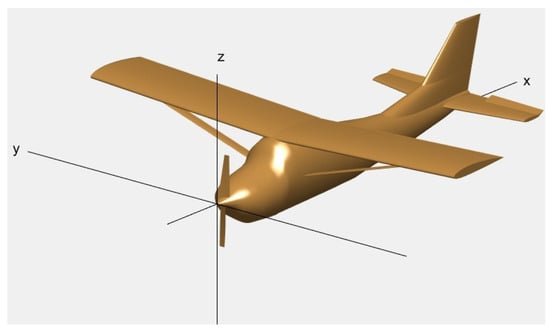
Figure 1.
Schematic of the UAV model.
By assuming that the UAV performs lateral maneuvering through bank-to-turn, and neglecting the effects of Earth’s rotation and flattening, the simplified centroid dynamic equations of a single UAV can be derived as follows [41]:
where x, y and z represent the position coordinates of the UAV in the inertial frame, m is the mass of the UAV, g is the local gravitational acceleration, V is the velocity, L and D are the lift and drag defined in the airflow frame, T represents the thrust, is the angle of attack, is the bank angle, and and are the trajectory inclination and declination, respectively.
For such low-speed aircraft, the aerodynamic forces (i.e., the lift L and drag D) can be written as [41]
where is the dynamic pressure, S represents the reference area. Within the flight envelope of the fixed-wing UAVs considered in this paper, the aerodynamic coefficients and can be modeled as [41]
where , , and are the parameters that can be calculated from aerodynamic data.
To facilitate subsequent research on the relative motion of UAVs, the velocity vector of UAVs is projected onto the inertial frame, thereby enabling the definition of , , and . Then Equations (1)–(3) can be simplified as
where and .
Since fixed-wing UAVs are incapable of hovering in the air, the motion can be divided into baseline motion and additional motion during the formation reconfiguration. For safety considerations, it is assumed that the process occurs in the cruise stage. Consequently, the baseline motion of a UAV is characterized by horizontal uniform-speed flight, during which aerodynamic forces, thrust, and gravity are in equilibrium. We define as the trim state, and as the state of additional motion. Notably, the relative motion frame maintains the trim state, with its initial position defined by the user. Then the kinematic equations of the additional motion can be derived as
Considering that this work centers on the formation control of UAVs, the attitude dynamics of UAVs is ignored for simplicity. Specifically, the inputs to the UAV system encompass the angle of attack , bank angle , and thrust T, while the outputs consist of the positions within the inertial coordinate framework.
2.3. Control Objectives
The objective of this study is to realize the automatic reconfiguration of the fixed-wing UAVs into a predefined configuration. The crux of this task lies in converging the current UAV formation to the desired configuration, which can be formulated as the following mathematical problem.
Define as the desired relative position of the i-th follower with respect to the leader. The deviations between the current formation configuration and the expected one can be quantified as the variable , viz.
where , , , and “=” holds if and only if the UAV formation converges to the expected configuration.
Taking the derivative with respect to time yields the dynamic model of
where , .
It can be found that if a control strategy is provided to ensure the convergence of the dynamic system from the given initial state to the origin, then the UAV formation reconstruction task can be accomplished. Therefore, the control problem for the formation reconfiguration of fixed-wing UAVs is formulated.
3. Preparations for Formation Reconfiguration Control
3.1. Control Framework Design
In the discussion in the previous section, the problem of formation reconfiguration control for fixed-wing UAVs has been formulated. It is worth emphasizing that this control process entails far more than merely designing distributed control laws. The process can be divided into the following steps: first, select the leader; second, determine the relative position of each UAV in the desired configuration; and finally, drive each UAV to its desired position. Therefore, the control framework for UAV formation reconfiguration can be designed as depicted in Figure 2. The contents, including control decision-making based on the SNG and auxiliary control systems, will be elaborated on in the next section.
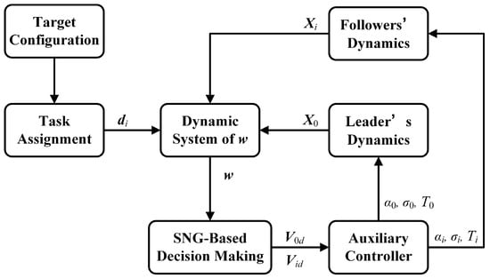
Figure 2.
The control framework for UAV formation reconfiguration.
3.2. Task Assignment
Prior to executing the formation reconfiguration task, it is essential to specify the destinations for each UAV. The first thing at this stage is to determine the position of the leader in the desired configuration. In general, the UAV positioned closest to the geometric center of the desired configuration is selected as the leader. This choice not only ensures a balanced spatial distribution but also facilitates more efficient communication with other UAVs.
Once the position of the leader within the desired configuration is determined, the relative positions of the followers can be therefore calculated (i.e., ; the order is user-defined). The challenge is then to sequentially match the UAVs with those in the desired configuration, that is, to determine the destination of each UAV. To reduce the adjustment complexity of the cluster and thereby lower the collision probability, the overall moving distance of the UAVs should be minimized. To acquire a reasonable task allocation scheme, the following optimization problem can be established.
Assign sequential initial indices to the UAVs, specifically . Manage to find the appropriate leader and the sequence such that the algebraic sum of displacements is minimized.
By solving the optimization problem (15), the leader’s index can be determined as . Simultaneously, the destinations for all the followers can be set via the correspondence between and . It is evident that the total number of leader–follower task allocation schemes amounts to . Therefore, when N is relatively small, the exhaustive method can be employed to solve the problem, whereas for larger values of N, it becomes necessary to consider incorporating swarm intelligence algorithms to address the increased complexity.
4. SNG-Based Leader–Follower Formation Reconfiguration Control
4.1. SNG-Based Optimal Control
After determining the relative positions of the UAVs in the desired configuration, the remaining task—also the most challenging part—is to ensure that the UAVs form the preset geometric shape. Following the goal of minimizing the moving distance proposed in Section 3, the value function can be defined as
where is the utility function of the i-th UAV.
Since the control process of the formation involves all the UAVs, the value function (16) of any UAV is inevitably influenced by the actions of other participants. Thus one can define the utility functions for the leader and followers as follows:
where , , , respectively represent the coupling coefficient matrices of the follower j with respect to the leader and the leader with respect to the follower j.
It should be noted that each UAV manages to adjust its control strategy to minimize its respective value function, which is interrelated with others. Consequently, the control decision-making process can be regarded as a multiplayer Stackelberg–Nash game. The following presents the relevant definitions.
Definition 1
(Best Response). A best response is the best decision a player can make to optimize the corresponding value function, given the strategies of the other players.
Definition 2
(Stackelberg–Nash Equilibrium). Define a mapping , and . If there exists a , such that for all ,
and simultaneously, if there exists a , such that for all ,
then is called the Stackelberg–Nash equilibrium.
Definition 3
(Multiplayer Stackelberg–Nash Game). If there exist appropriate strategies for all the players that stabilize the system (14) while constituting a Stackelberg–Nash equilibrium, then the leader and followers are said to be in a multiplayer Stackelberg–Nash game.
After transforming the issue into a multiplayer game problem, we then manage to solve the control decisions by employing the techniques of optimal control and policy iteration. At first we need to introduce the definitions of the optimal policy and its corresponding value function. For the leader,
For the followers,
where .
For all the players (), define the Hamiltonian as
where .
According to Definition 2, the optimal policy for the follower j is to minimize the value function (23) given the information of and , viz.,
where if .
Similarly, the optimal strategy for the leader can be derived by minimizing the value function (21) given the information of , viz.,
By applying the stationary condition, the optimal policies for the leader and the followers can be solved as
where with being an identity matrix.
It is worth noting that the optimal value functions satisfy the following coupled Hamilton–Jacobi–Bellman (HJB) equations:
and
where and .
The subsequent theorem guarantees that the strategies derived by solving the coupled HJB equations enable the UAV cluster to achieve Stackelberg–Nash equilibrium.
Theorem 1.
Consider the multiplayer SNG with the dynamic system (14). Let the functions be positive semi-definite and satisfy the HJB Equations (31) and (32). Suppose that the control policies for the leader and followers are given by Equations (29) and (30). Then the control policy profile is the Stackelberg–Nash equilibrium with the corresponding value function being , and the closed-loop system (14) is asymptotically stable.
Proof.
Stability: Consider as the Lyapunov candidate. Taking the derivative of along the trajectory , we have
This leads to the asymptotic stability of the closed-loop system.
Optimality: According to the assumed conditions, it can be deduced that
By utilizing contradiction, one can derive
The Hamiltonian can be rewritten as
From the definition, we have
Therefore, the profile constitutes the Stackelberg–Nash equilibrium, and is the optimal value function. This completes the proof. □
Although Theorem 1 shows that solving the coupled HJB Equations (31) and (32) can lead to the optimal control policies (29) and (30), this process involves considerable computational challenges. In the next subsection, an efficient algorithm is proposed to achieve the synchronous solution of the coupled HJB equations.
4.2. Leader–Follower Formation Control Algorithm
Let , which serves as a critical intermediate variable in deriving the optimal policy. Motivated by fixed-point iteration [39], the HJB Equations (31) and (32) can be rewritten in the following form:
where , and is a parameter.
Let , and . Note that one can calculate via the least square method, viz.
By adjusting the user-defined matrices and , one can ensure that for any , and . Once the above two conditions are satisfied, we can construct an iterative sequence eventually converging to . In other words, the coupled HJB Equations (31) and (32) can be solved via policy iteration, as presented in the subsequent algorithm.
Note that the approximate optimal policies obtained from Algorithm 1 represent the desired velocities for the UAVs’ additional motions. To enable UAVs to complete the formation reconfiguration task, it is essential to translate these commands into executable actions, specifically thrust, angle of attack, and tilt angle. This will be detailed in the subsequent section.
| Algorithm 1 Policy iteration algorithm for multiplayer Stackelberg–Nash game |
|
4.3. Auxiliary Controller Design
In the subsequent discussion, to avoid ambiguity, the desired velocity for the additional motions calculated by Algorithm 1 is denoted as . Given the cruising velocity , the expected velocity for the i-th UAV can be determined by
By converting the expected velocity for the i-th UAV into the trajectory frame, one can obtain
It is worth noting that there are two approaches to solving in order to prevent singularity.
Define as the normalized tracking error
Then a PD controller can be designed to achieve the tracking control of the desired velocity for each UAV, viz.
where , and are the PD controller gains.
Therefore, we can conclude the algorithm for the UAV formation reconfiguration control in Algorithm 2.
| Algorithm 2 SNG-based control algorithm for the UAV formation reconfiguration |
|
Remark 1.
Due to the similarity of the performance functions among the followers, adding an additional follower does not substantially increase the calculation time of Algorithm 1. Nevertheless, the computational complexity of the task allocation problem exhibits a “dimension curse” as the number of followers increases; thus, the number of UAVs cannot be expanded indefinitely.
5. Simulation Results
In this section, numerical simulations will be conducted to validate the effectiveness of the proposed scheme for UAV formation reconfiguration.
The relevant parameters of the model, flight, and aerodynamic coefficients are presented in Table 1, Table 2 and Table 3, respectively. The external dimensions of the original Cessna 172 are provided in [42]. In this paper, the aircraft is scaled down and utilized as the fixed-wing UAVs. The center of mass is positioned at 37% of the length from the nose of the aircraft, which is ahead of the aerodynamic focus, thereby ensuring the static stability. The fight scenarios presented in Table 2 are user-defined. This article sets the flight altitude at approximately 500 m, primarily considering that cruising at this altitude is well-suited for tasks such as fire warning. The trim angle and thrust are calculated based on the cruising state and aerodynamic coefficients given in Table 3. Since all the UAVs are in a cruising state in the beginning, the initial bank angle is set to 0 deg. It should be particularly noted that the aerodynamic parameters are generated using the aerodynamic analysis software Tornado.

Table 1.
Model parameters.
Table 2.
Fight parameters.
Table 3.
Aerodynamic coefficients.
Assume that the total number of UAVs is 7. Set the initial positions of the UAVs numbered to in the inertial frame as
m, m, m, m, m, m, m.
The desired formation configuration is an approximate regular hexagon in a horizontal plane and the leader is located at the geometry center. Set the expected relative positions with respect to the leader as
, , , , , .
Other relevant parameter settings are as follows. We choose , , and , where . The gains of the auxiliary control system is set to and . The thresholds related to the termination of Algorithm 1 and Algorithm 2 are set to and , respectively.
Based on the initial positions of the UAVs and the desired configuration, the exhaustive method, which involves a total of possible combinations, is employed for task allocation. By solving the optimization problem (15), the UAV originally numbered s4 was determined as the leader. The corresponding relationships between the other original numbers and new numbers are , , , , , and .
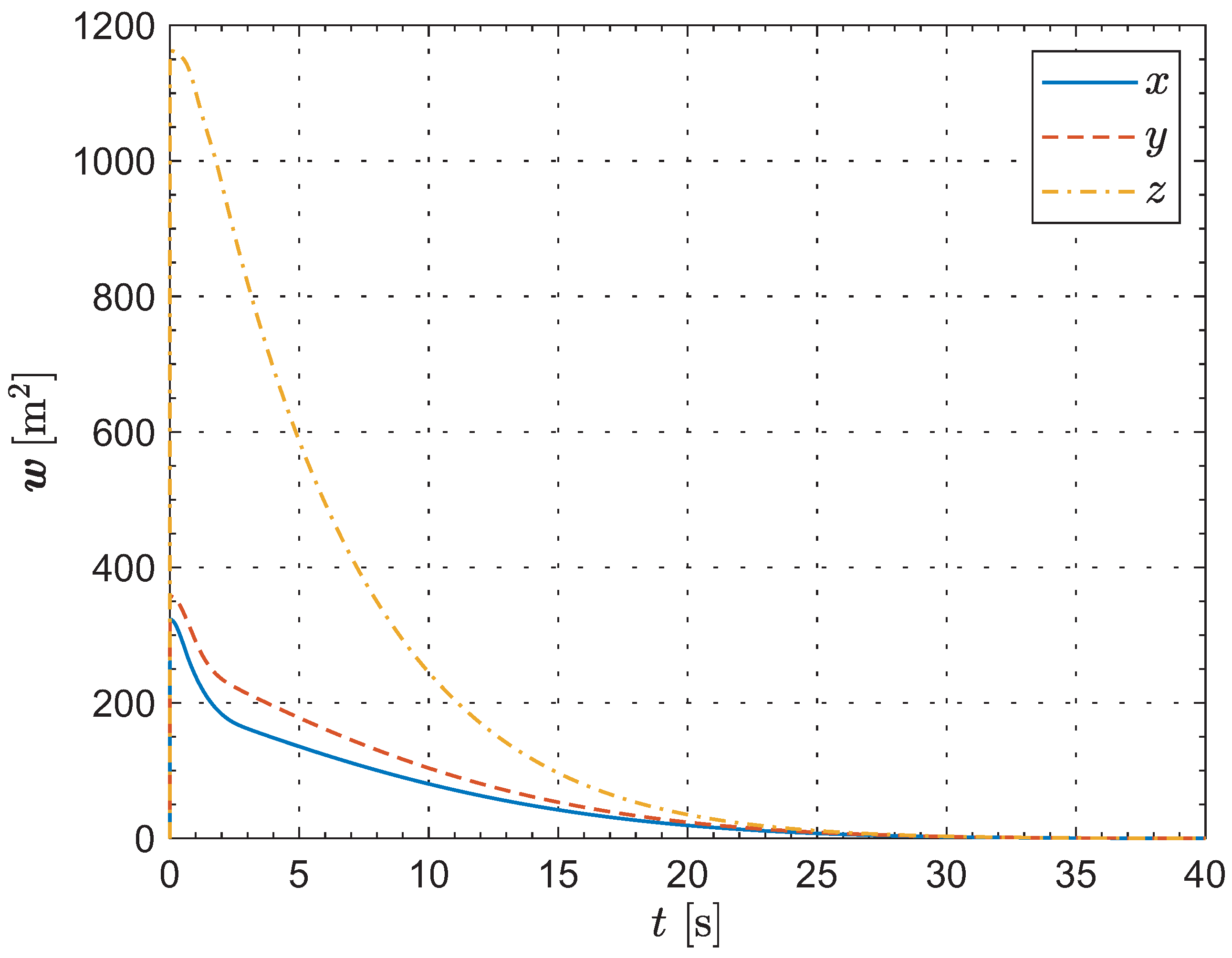
Next, the computer simulation of the formation reconfiguration is conducted using the MATLAB R2024a platform. Figure 3 illustrates the deviations between the current formation configuration and the desired configuration. As can be seen from the evolution of the key indicator , at the initial moment, the projections on the directions of the inertial coordinate frame are , and , respectively. As defined earlier, since represents the sum of the squares of the relative distances in the three directions, it is always non-negative, and the unit is . As time progresses, rapidly decreases in all three directions until it converges to within at 33.54, which corresponds to the termination condition of Algorithm 2. At 40 s, this indicator reaches . Thus, we can conclude that the deviations between the current formation configuration and the desired configuration gradually converge to zero over time.
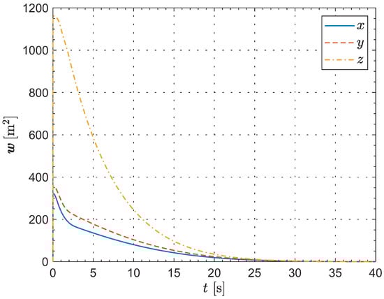
Figure 3.
The deviations between the current formation configuration and the desired configuration.
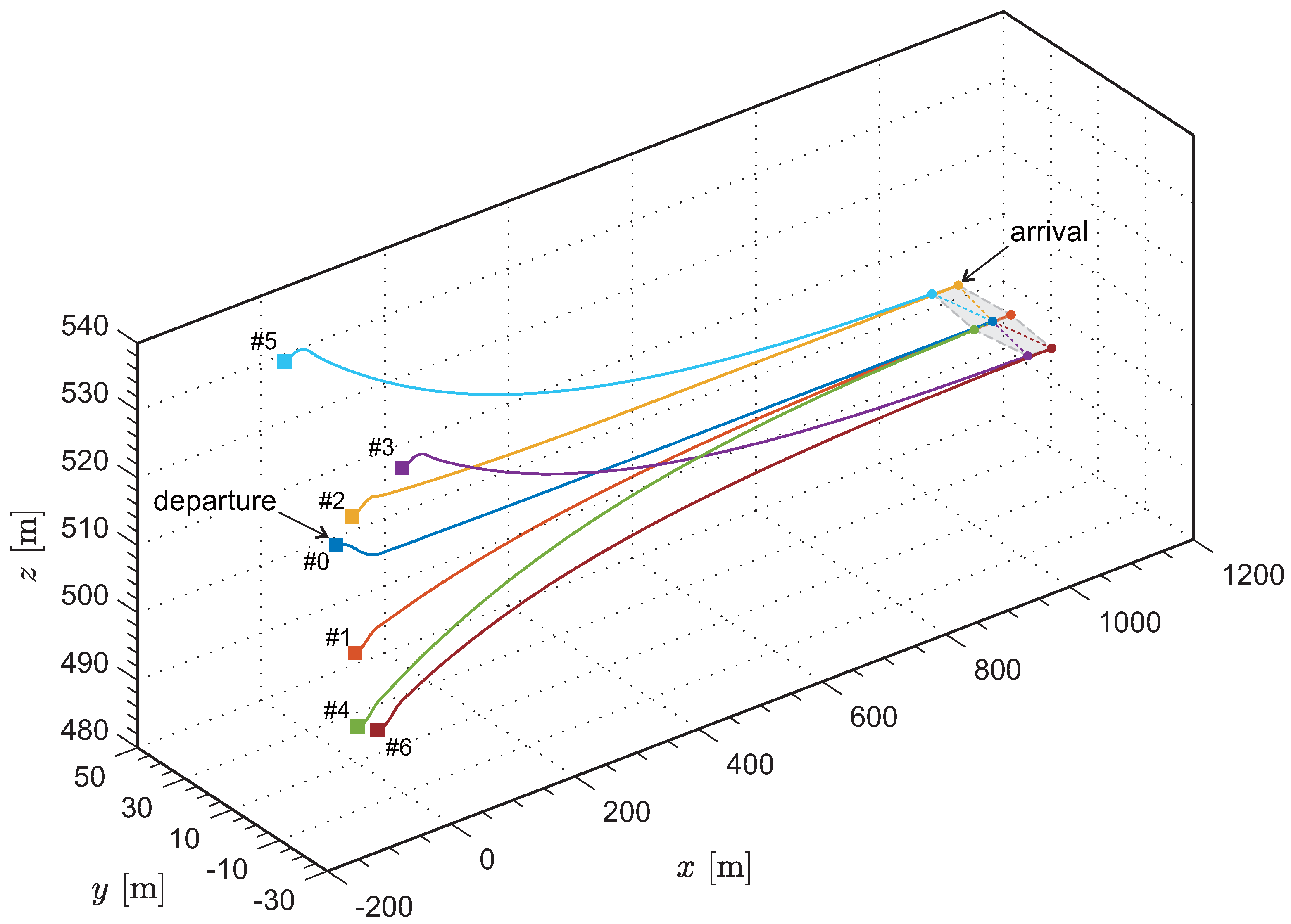
Figure 4 presents the flight trajectories of the fixed-wing UAVs in the inertial frame. For aesthetic purposes, the image is moderately stretched in the y and z directions. After the departure, within a distance ahead, the UAV formation transitions to the predetermined configuration. The entire reconfiguration process is completed while in motion, and the flight trajectory of each UAV remains relatively smooth.
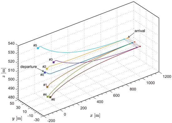
Figure 4.
Three–dimensional flight trajectories of the fixed-wing UAVs in the inertial frame.
Figure 5 illustrates the 3D trajectories from the perspective of relative motion. The reference point of the relative motion frame is located at the initial position , and the moving velocity remains constant at . The relative motion trajectories further corroborate that the UAVs precisely execute the flight plan, successfully achieving the predetermined configuration. It is noted that the flight trajectories do not show any crossing or close contact, which indicates that a safe distance is maintained between the UAVs throughout the entire flight process.
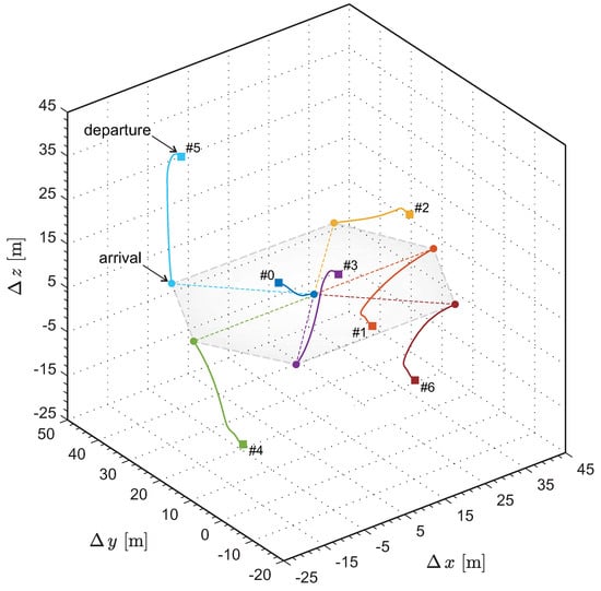
Figure 5.
Three–dimensional flight trajectories of the fixed-wing UAVs in the relative motion frame.
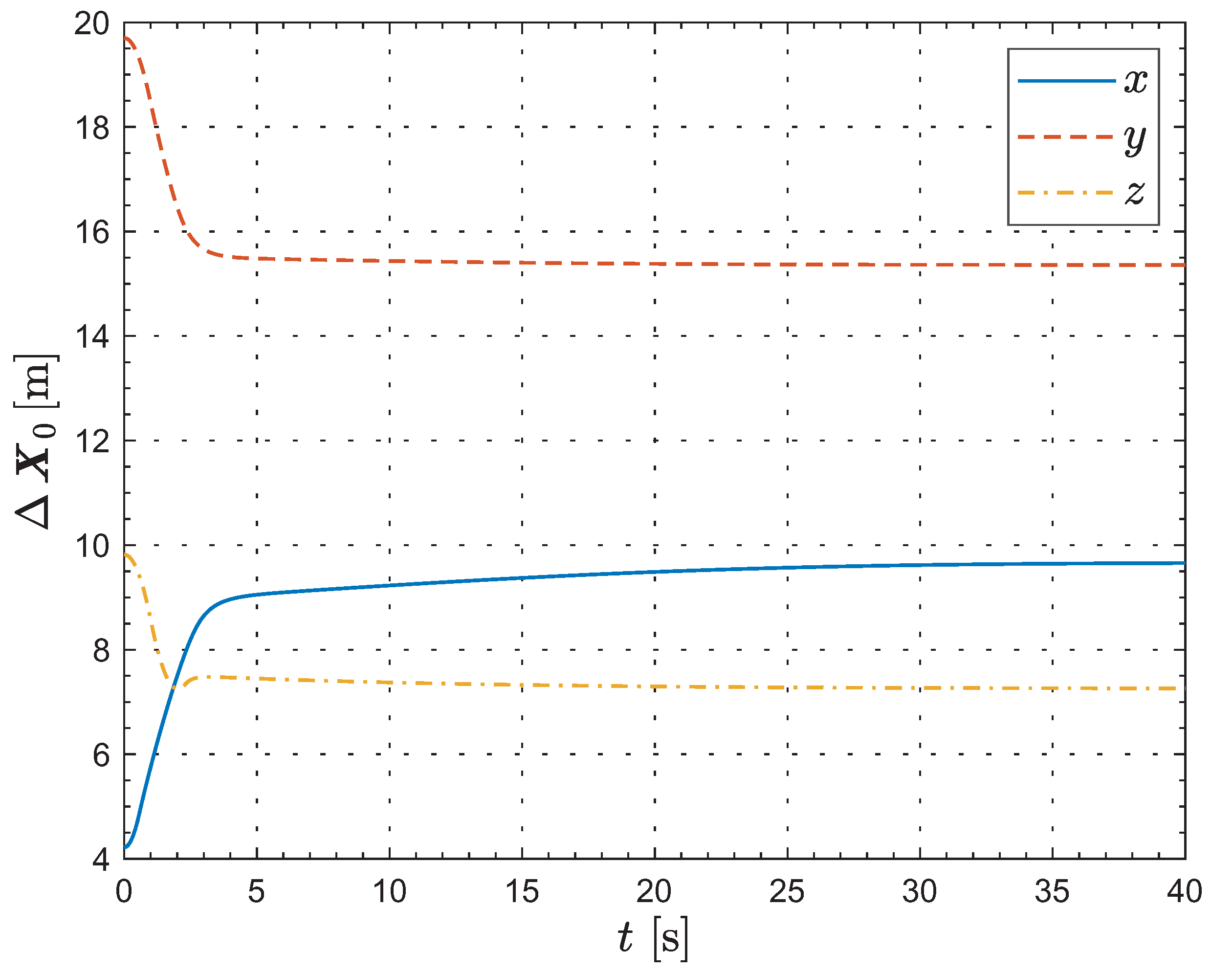
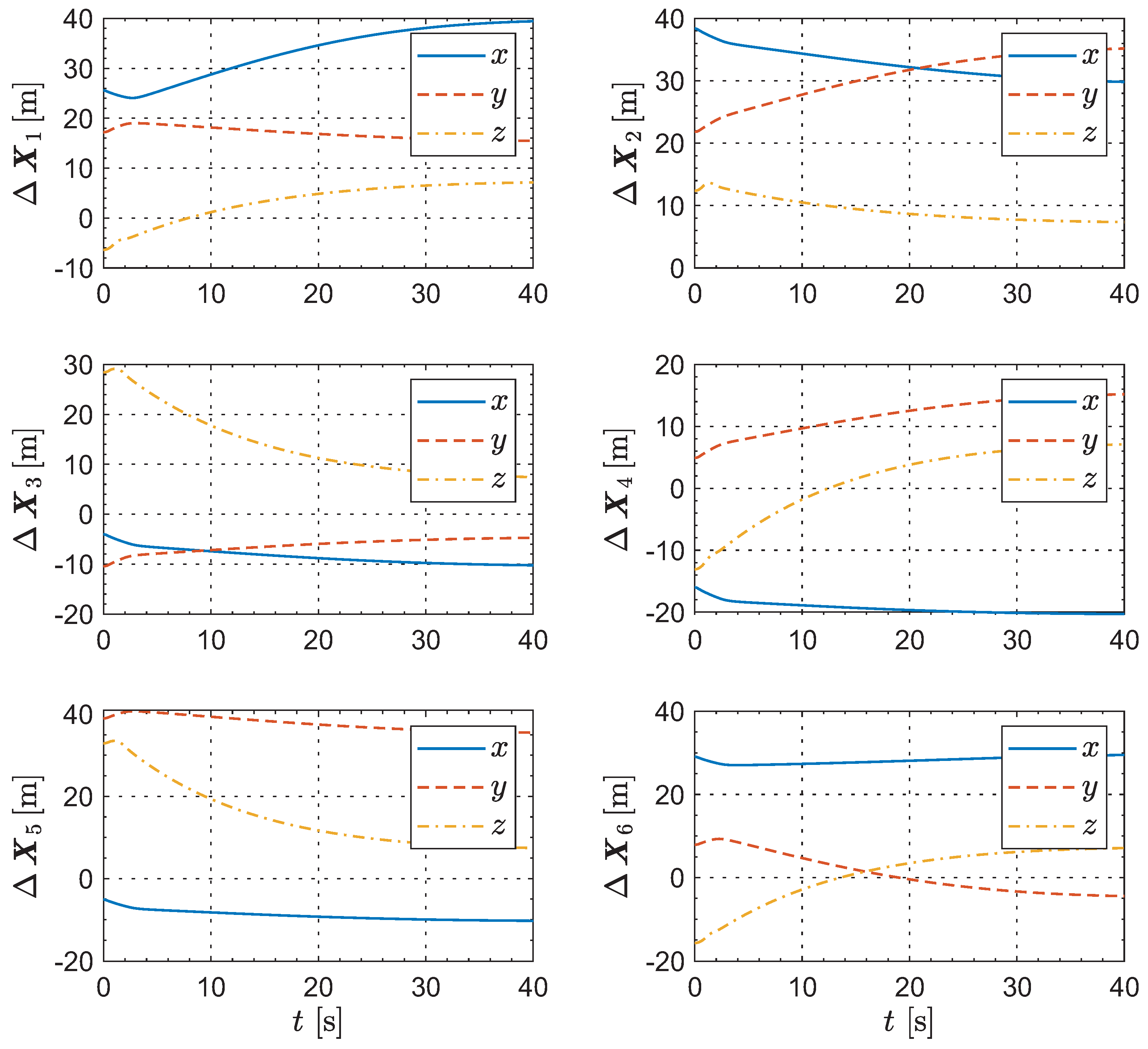
The coordinates of the leader and the followers in the relative motion frame are respectively given by Figure 6 and Figure 7. As can be observed from these several groups of “position–time” curves, following the trajectory adjustment, the UAVs eventually become relatively static, thereby forming a stable geometric configuration. It is worth noting that there is almost no overshoot in any of the UAV trajectories. This outcome arises from the independent decision-making process of each UAV aimed at achieving its shortest path, further indicating the optimality of the method proposed in this paper.
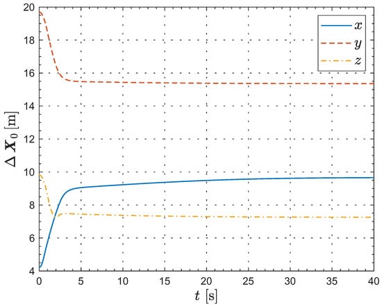
Figure 6.
The evolution of the leader’s coordinates in the relative motion frame.
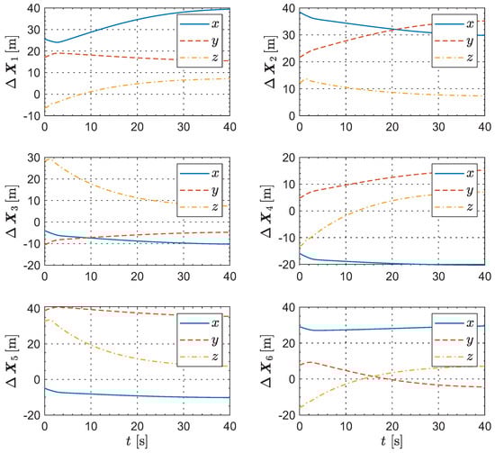
Figure 7.
The evolution of the followers’ coordinates in the relative motion frame.
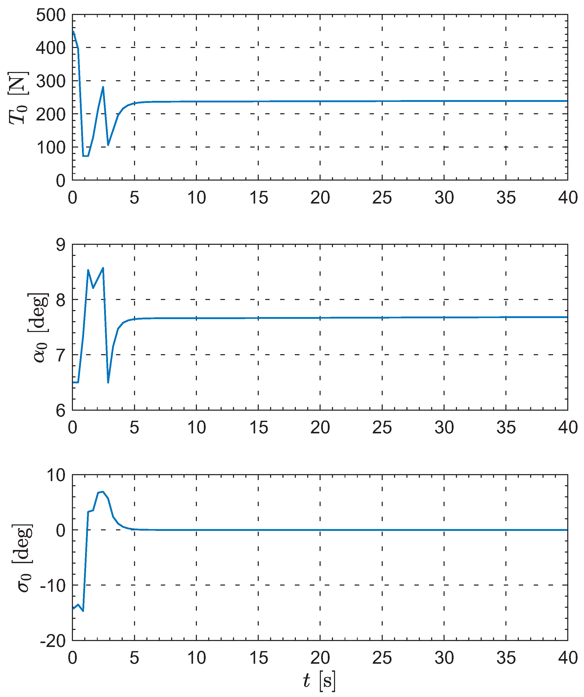
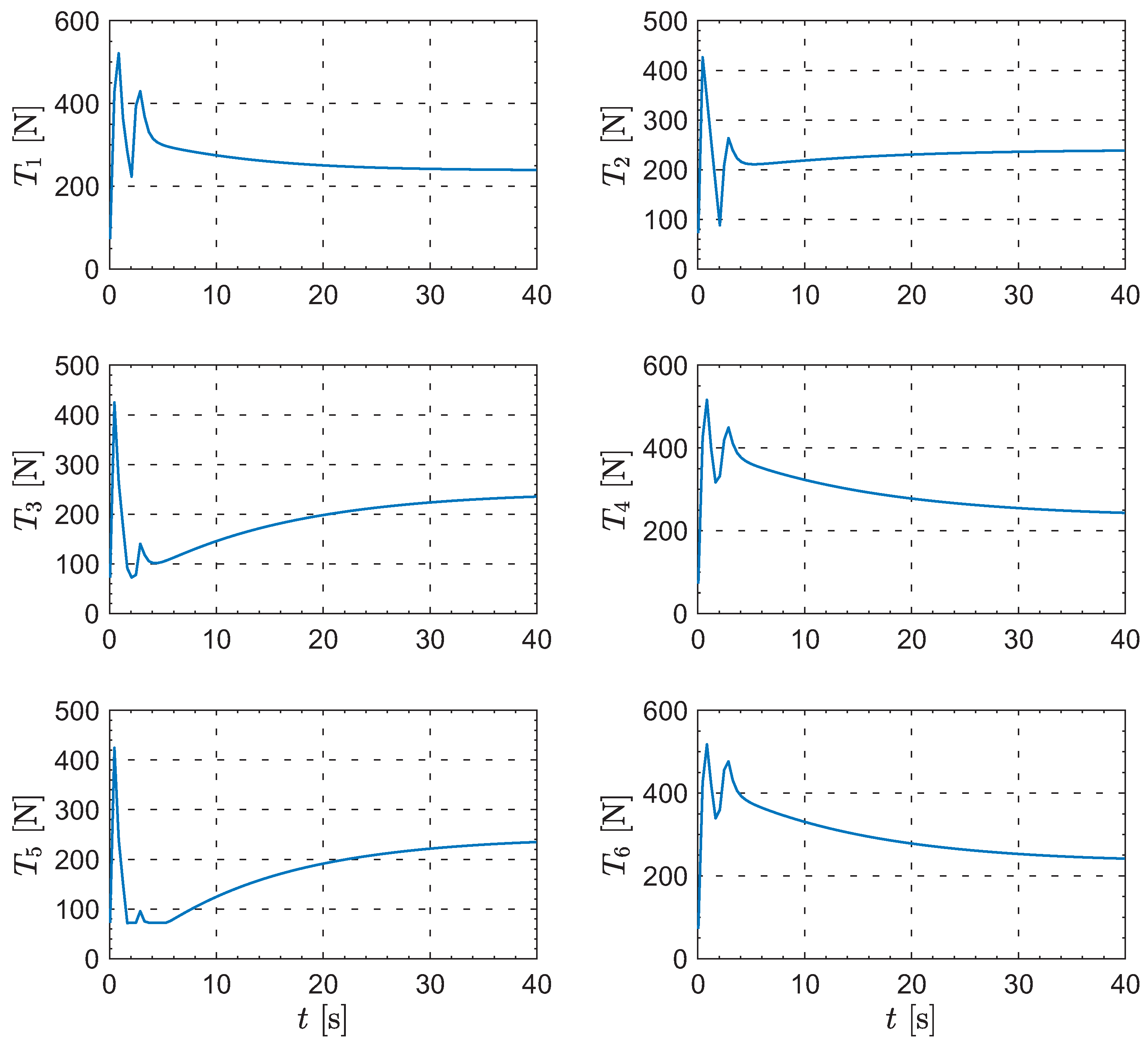
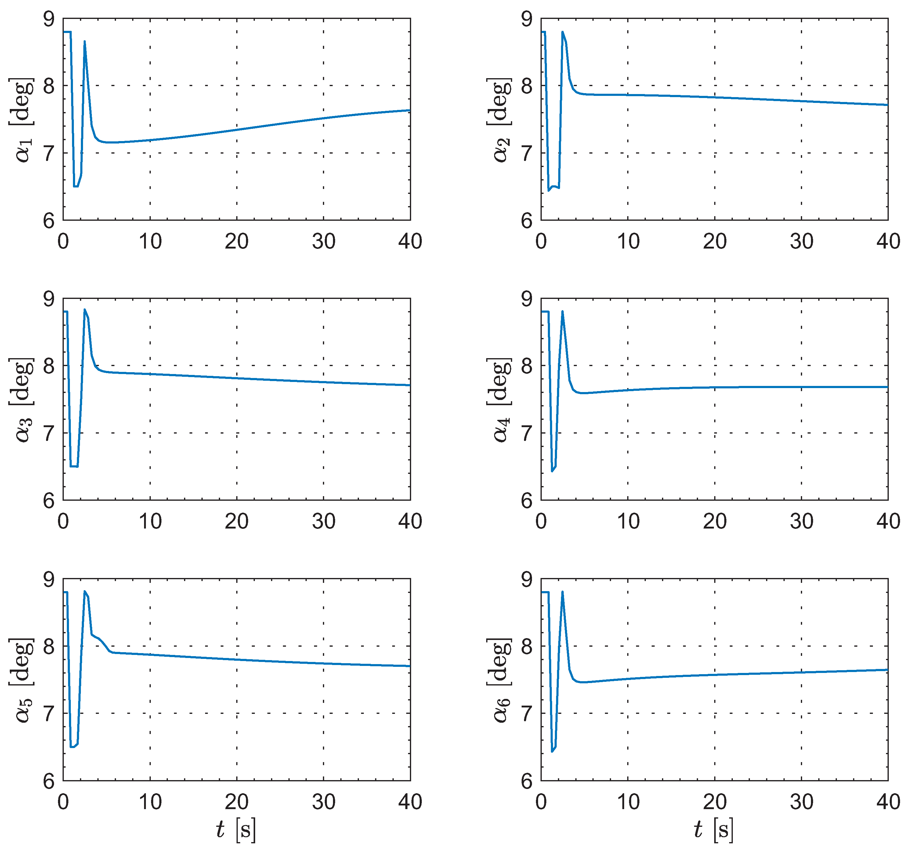
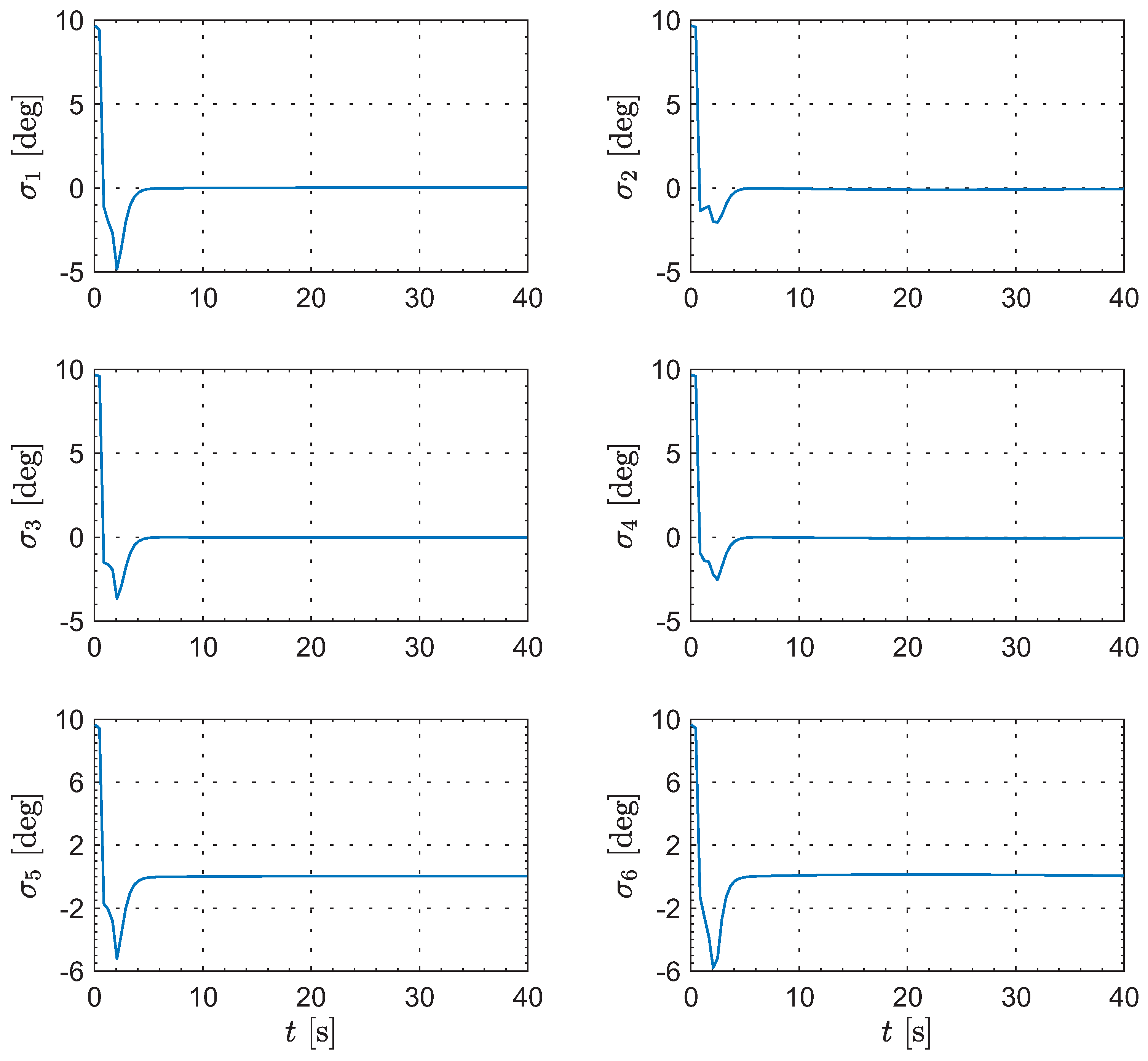
Moreover, Figure 8, Figure 9, Figure 10 and Figure 11 show the control inputs for the leader and followers during the formation reconfiguration stage, specifically including thrust T, angle of attack , and bank angle . As can be seen in these figures, the control inputs remain executable and eventually converge to their respective trim values.
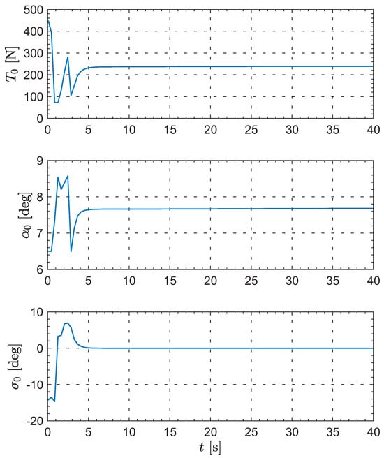
Figure 8.
The evolution of the leader’s inputs.
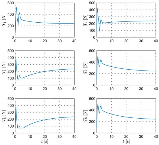
Figure 9.
The evolution of the followers’ thrust.
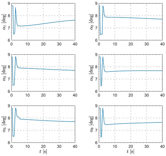
Figure 10.
The evolution of the followers’ angle of attack.
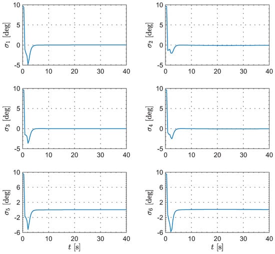
Figure 11.
The evolution of the followers’ bank angle.
6. Conclusions
This article studies the control strategies for formation reconfiguration of fixed-wing UAVs. In particular, a PI-based hierarchical control algorithm (i.e., Algorithm 1) is proposed to address the multiplayer SNG problem, and on this basis, a formation decision-making framework is established. To accurately implement the speed commands generated by the algorithm, an auxiliary control subsystem is developed, thereby ensuring the stable operation of the leader–follower flight control system. Furthermore, a task allocation mechanism has been constructed for the UAV swarm, thus laying a solid foundation for subsequent formation control. Specifically, based on the initial distribution of the UAVs and information of the desired configuration, with the shortest path serving as the indicator, the destinations of the UAVs are therefore determined.
This paper marks the beginning of our research on formation reconfiguration and optimal control, focusing on proposing a hierarchical decision-making framework for achieving the shortest path and conducting a theoretical analysis of the scheme’s feasibility. Owing to space constraints, we do not account for the information transmission delay, or external disturbances such as gusts and turbulence. These factors will be progressively addressed in our future research.
Author Contributions
Conceptualization, H.Z.; methodology, H.Z.; software, H.Z.; validation, H.Z.; formal analysis, H.Z.; investigation, H.Z.; resources, H.Z.; data curation, H.Z.; writing—original draft preparation, H.Z.; writing—review and editing, H.Z.; visualization, H.Z.; supervision, S.W.; project administration, S.W.; funding acquisition, S.W. All authors have read and agreed to the published version of the manuscript.
Funding
This work was supported by the National Natural Science Foundation of China (grant no. U24B6014).
Data Availability Statement
The original contributions presented in this study are included in the article. Further inquiries can be directed to the corresponding author.
DURC Statement
The current research is limited to UAV guidance and control, which is beneficial for civilian areas, including emergency rescue, coastal surveying and fire monitoring, and does not pose a threat to public health or national security. The authors acknowledge the dual-use potential of the research involving UAV guidance and control and confirm that all necessary precautions (e.g., using non-realistic UAV models and virtual aerodynamic data) have been taken to prevent potential misuse. As an ethical responsibility, the authors strictly adhere to relevant national and international laws about DURC. The authors advocate for responsible deployment, ethical considerations, regulatory compliance, and transparent reporting to mitigate misuse risks and foster beneficial outcomes.
Conflicts of Interest
The authors declare no conflicts of interest.
Abbreviations
The following abbreviations are used in this manuscript:
| UAV | Unmanned aerial vehicle |
| SNG | Stackelberg–Nash game |
| PI | Policy iteration |
| PD | Proportional plus derivative controller |
References
- Ghamari, M.; Rangel, P.; Mehrubeoglu, M.; Tewolde, G.S.; Sherratt, R.S. Unmanned aerial vehicle communications for civil applications: A review. IEEE Access 2022, 10, 102492–102531. [Google Scholar] [CrossRef]
- Zhao, N.; Lu, W.; Sheng, M.; Chen, Y.; Tang, J.; Yu, F.R.; Wong, K.K. UAV-assisted emergency networks in disasters. IEEE Wirel. Commun. 2019, 26, 45–51. [Google Scholar] [CrossRef]
- Tang, P.; Li, J.; Sun, H. A review of electric UAV visual detection and navigation technologies for emergency rescue missions. Sustainability 2024, 16, 2105. [Google Scholar] [CrossRef]
- Turner, I.L.; Harley, M.D.; Drummond, C.D. UAVs for coastal surveying. Coast. Eng. 2016, 114, 19–24. [Google Scholar] [CrossRef]
- Casbeer, D.W.; Beard, R.W.; McLain, T.W.; Li, S.M.; Mehra, R.K. Forest fire monitoring with multiple small UAVs. In Proceedings of the 2005, American Control Conference, Portland, OR, USA, 8–10 June 2005; IEEE: Piscataway, NJ, USA, 2005; pp. 3530–3535. [Google Scholar]
- Hu, J.; Niu, H.; Carrasco, J.; Lennox, B.; Arvin, F. Fault-tolerant cooperative navigation of networked UAV swarms for forest fire monitoring. Aerosp. Sci. Technol. 2022, 123, 107494. [Google Scholar] [CrossRef]
- Jafari, B.; Saeedi, H.; Pishro-Nik, H. UAV Path Planning for Surveillance Applications: Rotary-Wing vs. Fixed-Wing UAVs. In Proceedings of the 2024 IEEE 99th Vehicular Technology Conference (VTC2024-Spring), Singapore, 24–27 June 2024; IEEE: Piscataway, NJ, USA, 2024; pp. 1–6. [Google Scholar]
- Lyu, M.; Zhao, Y.; Huang, C.; Huang, H. Unmanned aerial vehicles for search and rescue: A survey. Remote Sens. 2023, 15, 3266. [Google Scholar] [CrossRef]
- Yang, Z.; Yang, F.; Mao, T.; Xiao, Z.; Han, Z.; Xia, X. Reconfiguration for UAV formation: A novel method based on modified artificial bee colony algorithm. Drones 2023, 7, 595. [Google Scholar] [CrossRef]
- Kim, M.H.; Baik, H.; Lee, S. Resource welfare based task allocation for UAV team with resource constraints. J. Intell. Robot. Syst. 2015, 77, 611–627. [Google Scholar] [CrossRef]
- Yang, Y.; Xiong, X.; Yan, Y. UAV formation trajectory planning algorithms: A review. Drones 2023, 7, 62. [Google Scholar] [CrossRef]
- Du, Z.; Zhang, H.; Wang, Z.; Yan, H. Model predictive formation tracking-containment control for multi-UAVs with obstacle avoidance. IEEE Trans. Syst. Man, Cybern. Syst. 2024, 54, 3404–3414. [Google Scholar] [CrossRef]
- Evangeliou, N.; Chaikalis, D.; Tsoukalas, A.; Tzes, A. Visual collaboration leader-follower UAV-formation for indoor exploration. Front. Robot. AI 2022, 8, 777535. [Google Scholar] [CrossRef] [PubMed]
- Li, J.; Liu, J.; Huangfu, S.; Cao, G.; Yu, D. Leader-follower formation of light-weight UAVs with novel active disturbance rejection control. Appl. Math. Model. 2023, 117, 577–591. [Google Scholar] [CrossRef]
- Askari, A.; Mortazavi, M.; Talebi, H. UAV formation control via the virtual structure approach. J. Aerosp. Eng. 2015, 28, 04014047. [Google Scholar] [CrossRef]
- Cai, Z.; Liu, Y.; Zhao, J.; Wang, Y. Virtual structure and artificial potential field-based cooperative control for uav formation. In Advances in Guidance, Navigation and Control; Springer: Berlin/Heidelberg, Germany, 2022; pp. 366–375. [Google Scholar]
- Liu, Y.; Liu, Z.; Wang, G.; Yan, C.; Wang, X.; Huang, Z. Flexible multi-UAV formation control via integrating deep reinforcement learning and affine transformations. In Aerospace Science and Technology; Elsevier: Amsterdam, The Netherlands, 2024; p. 109812. [Google Scholar]
- Ma, B.; Liu, Z.; Jiang, F.; Zhao, W.; Dang, Q.; Wang, X.; Zhang, J.; Wang, L. Reinforcement learning based UAV formation control in GPS-denied environment. Chin. J. Aeronaut. 2023, 36, 281–296. [Google Scholar] [CrossRef]
- Bu, Y.; Yan, Y.; Yang, Y. Advancement challenges in UAV swarm formation control: A comprehensive review. Drones 2024, 8, 320. [Google Scholar] [CrossRef]
- Zhu, L.; Ma, C.; Li, J.; Lu, Y.; Yang, Q. Connectivity-maintenance UAV formation control in complex environment. Drones 2023, 7, 229. [Google Scholar] [CrossRef]
- Du, Z.; Qu, X.; Shi, J.; Lu, J. Formation control of fixed-wing UAVs with communication delay. ISA Trans. 2024, 146, 154–164. [Google Scholar] [CrossRef]
- Tong, W.; Jie, W.; Bailing, T. Periodic event-triggered formation control for multi-UAV systems with collision avoidance. Chin. J. Aeronaut. 2022, 35, 193–203. [Google Scholar]
- Raza, S.A.; Etele, J. Autonomous position control analysis of quadrotor flight in urban wind gust conditions. In Proceedings of the AIAA Guidance, Navigation, and Control Conference, San Diego, CA, USA, 4–8 January 2016; p. 1385. [Google Scholar]
- Saska, M.; Hert, D.; Baca, T.; Kratky, V.; Nascimento, T. Formation control of unmanned micro aerial vehicles for straitened environments. Auton. Robot. 2020, 44, 991–1008. [Google Scholar] [CrossRef]
- Hu, J.; Wang, M.; Zhao, C.; Pan, Q.; Du, C. Formation control and collision avoidance for multi-UAV systems based on Voronoi partition. Sci. China Technol. Sci. 2020, 63, 65–72. [Google Scholar] [CrossRef]
- Li, M.; Qin, J.; Freris, N.M.; Ho, D.W. Multiplayer Stackelberg–Nash game for nonlinear system via value iteration-based integral reinforcement learning. IEEE Trans. Neural Netw. Learn. Syst. 2020, 33, 1429–1440. [Google Scholar] [CrossRef] [PubMed]
- Simaan, M.; Cruz, J.B., Jr. On the Stackelberg strategy in nonzero-sum games. J. Optim. Theory Appl. 1973, 11, 533–555. [Google Scholar] [CrossRef]
- Bagchi, A.; Başar, T. Stackelberg strategies in linear-quadratic stochastic differential games. J. Optim. Theory Appl. 1981, 35, 443–464. [Google Scholar] [CrossRef]
- Bensoussan, A.; Chen, S.; Sethi, S.P. The maximum principle for global solutions of stochastic Stackelberg differential games. SIAM J. Control Optim. 2015, 53, 1956–1981. [Google Scholar] [CrossRef]
- Zheng, Y.; Shi, J. A Stackelberg game of backward stochastic differential equations with applications. Dyn. Games Appl. 2020, 10, 968–992. [Google Scholar] [CrossRef]
- Xu, J.; Zhang, H. Sufficient and necessary open-loop Stackelberg strategy for two-player game with time delay. IEEE Trans. Cybern. 2015, 46, 438–449. [Google Scholar] [CrossRef]
- Meng, Y.; Liu, C.; Liu, Y.; Tan, L. Adaptive fault-tolerant control for spacecraft: A dynamic Stackelberg game approach with advantage actor-critic reinforcement learning. Aerosp. Sci. Technol. 2024, 154, 109522. [Google Scholar] [CrossRef]
- Lin, Y.; Jiang, X.; Zhang, W. An open-loop Stackelberg strategy for the linear quadratic mean-field stochastic differential game. IEEE Trans. Autom. Control 2018, 64, 97–110. [Google Scholar] [CrossRef]
- Ming, Z.; Zhang, H.; Yan, Y.; Yang, L. Adaptive Optimal Control via Q-Learning for Itô Fuzzy Stochastic Nonlinear Continuous-Time Systems With Stackelberg Game. IEEE Trans. Fuzzy Syst. 2024, 32, 2029–2038. [Google Scholar]
- Lin, M.; Zhao, B.; Liu, D.; Zhang, Y. Policy iteration adaptive dynamic programming for optimal control of multi-player Stackelberg-Nash games. In Proceedings of the 2022 41st Chinese Control Conference (CCC), Hefei, China, 25–27 July 2022; IEEE: Piscataway, NJ, USA, 2022; pp. 2393–2397. [Google Scholar]
- Yu, M.; Hong, S.H. A real-time demand-response algorithm for smart grids: A stackelberg game approach. IEEE Trans. Smart Grid 2015, 7, 879–888. [Google Scholar] [CrossRef]
- Yu, K.; Li, Y.; Lv, M.; Tong, S. Distributed Optimal Formation Control of Multiple Unmanned Surface Vehicles with Stackelberg Differential Graphical Game. In IEEE Transactions on Artificial Intelligence; IEEE: Piscataway, NJ, USA, 2024; pp. 4058–4073. [Google Scholar]
- Zhang, Y.; Zhang, P.; Wang, X.; Song, F.; Li, C.; Hao, J. An open loop Stackelberg solution to optimal strategy for UAV pursuit-evasion game. Aerosp. Sci. Technol. 2022, 129, 107840. [Google Scholar] [CrossRef]
- Borwein, J.M.; Li, G.; Tam, M.K. Convergence rate analysis for averaged fixed point iterations in common fixed point problems. SIAM J. Optim. 2017, 27, 1–33. [Google Scholar] [CrossRef]
- Zarchan, P. Tactical and Strategic Missile Guidance; American Institute of Aeronautics and Astronautics, Inc.: Reston, VA, USA, 2012. [Google Scholar]
- Stengel, R.F. Flight Dynamics; Princeton University Press: Princeton, NJ, USA, 2005. [Google Scholar]
- Smith, R. Cessna 172: A Pocket History; Amberley Publishing Limited: Gloucestershire, UK, 2010. [Google Scholar]


Disclaimer/Publisher’s Note: The statements, opinions and data contained in all publications are solely those of the individual author(s) and contributor(s) and not of MDPI and/or the editor(s). MDPI and/or the editor(s) disclaim responsibility for any injury to people or property resulting from any ideas, methods, instructions or products referred to in the content. |
© 2025 by the authors. Licensee MDPI, Basel, Switzerland. This article is an open access article distributed under the terms and conditions of the Creative Commons Attribution (CC BY) license (https://creativecommons.org/licenses/by/4.0/).