Robust Tracking Control of Underactuated UAVs Based on Zero-Sum Differential Games

Abstract

This paper investigates the robust tracking control of unmanned aerial vehicles (UAVs) against external time-varying disturbances. First, by introducing a virtual position controller, we innovatively decouple the UAV dynamics into independent position and attitude error subsystems, transforming the robust tracking problem into two zero-sum differential games. This approach contrasts with conventional methods by treating disturbances as strategic “players”, enabling a systematic framework to address both external disturbances and model uncertainties. Second, we develop an integral reinforcement learning (IRL) framework that approximates the optimal solution to the Hamilton–Jacobi–Isaacs (HJI) equations without relying on precise system models. This model-free strategy overcomes the limitation of traditional robust control methods that require known disturbance bounds or accurate dynamics, offering superior adaptability to complex environments. Third, the proposed recursive Ridge regression with a forgetting factor (${\mathrm{R}}^3{\mathrm{F}}^2$ ) algorithm updates actor-critic-disturbance neural network (NN) weights in real time, ensuring both computational efficiency and convergence stability. Theoretical analyses rigorously prove the closed-loop system stability and algorithm convergence, which fills a gap in existing data-driven control studies lacking rigorous stability guarantees. Finally, numerical results validate that the method outperforms state-of-the-art model-based and model-free approaches in tracking accuracy and disturbance rejection, demonstrating its practical utility for engineering applications.

1. Introduction

Unmanned aerial vehicles (UAVs) have drawn increasing research interest and have been applied to many complex tasks, e.g., surveillance, firefighting, environmental monitoring, etc., mainly due to several advantages such as simple mechanisms, flexible mobility, and the ability to vertically hover and take off [1,2,3,4,5,6]. However, it may pose challenges to designing a robust optimal tracking controller for UAVs in a dynamic and complex environment. In typical application scenarios, UAVs inherently exhibit a mismatch between control inputs and degrees of freedom (e.g., four control inputs regulating six degrees of freedom), leading to strong coupling between position and attitude control. Furthermore, external time-varying disturbances (e.g., airflow disturbances), model parameter perturbations, and unmodeled dynamics further exacerbate the control complexity. Various classic robust control methods and technologies have been applied to address the aforementioned issues, e.g., ${\mathcal{H}}_{\infty }$ control [7], backstepping control [8], adaptive control [9], and model predictive control [10]. These kinds of underactuated systems pose dual requirements for control precision and robustness, which makes the existing control methods based on perfect model assumptions difficult to handle. Although the actor-critic algorithm solves the policy interaction problem, it does not involve the handling of physical system dynamics and uncertainties, and therefore cannot be directly applied to the robust tracking control of UAV systems.

To address the issues, a combination of zero-sum differential game and reinforcement learning (RL) has recently drawn increasing research interest [11,12,13]. Game theory provides an effective solution for such problems [11], which models the interaction between the system and uncertainty as a dynamic game process. The external disturbances, parameter perturbations, and other uncertainties are modeled as an “adversary”, while the control strategy is modeled as a “defender” countering them, constructing a dynamic adversarial relationship between optimal control and the worst-case disturbance. Robust control strategies [14,15] designed based on this theoretical framework can obtain optimal control strategies through game equilibrium solutions, considering extreme disturbance scenarios, and are naturally adapted to the dual requirements of underactuated systems for strong robustness and high-precision tracking. Reinforcement learning enables agents to select the optimal action or control strategy based on the observed system responses in order to maximize or minimize the cumulative reward. In recent years, RL and deep reinforcement learning (DRL) technologies have been widely used in UAV control problems. For instance, the authors of [12] proposed a deep neural network (DNN) called TrailNet, which was applied to the tracking control of micro air vehicles (MAVs) in an unstructured outdoor environment (e.g., mountainous areas, forests, jungles, etc.). A deep deterministic policy gradient (DDPG) algorithm for UAV trajectory tracking in a simulation environment was investigated in [16]. In [17], an RL method was applied to the fault-tolerant controller design problem for an unknown nonlinear UAV with actuator faults. In [18], an RL-based MPC approach was developed for UAV navigation control in unknown environments, where both the vehicle control and obstacle avoidance tasks were fulfilled using MPC, whereas the guidance of the MAV through complex environments was completed by RL. In [19], a model-based adaptive dynamic programming (ADP) was designed for solving the UAV robust tracking control problem under coupling uncertainties. Moreover, the DRL-based robust control problem for UAV helicopters was studied in [13].

Integral RL (IRL) [20] is an integral temporal difference-based RL methodology, which is provably effective in solving the optimal control and decision-making problems of nonlinear systems with partially known or completely unknown system dynamics. To relieve the demand for knowing the system model, the IRL scheme aims to design the optimal robust controller by solving the integral Bellman equations via the policy iteration (PI) technique. Among the existing literature, the proposed IRL-based robust tracking control methods typically use three NN-based architectures, as follows: critic neural networks (NNs), actor-critic NNs, and actor-critic-disturbance NNs. For instance, Wang et al. [21] proposed a neural identifier-based intelligent critic control for unknown nonlinear affine dynamics to achieve disturbance attenuation. In [22], nonlinear disturbance-observer-based critic NNs were used to solve the problem of cooperative control for nonlinear dynamical systems under mismatched disturbances. Motivated by [22], Mohammadi et al. [23] proposed a value-iteration-based algorithm for optimal tracking control of nonlinear dynamical systems subject to delays, disturbances, and constraints. In [24], Yang et al. developed a critic NN-based event-driven robust controller for continuous-time (CT) nonlinear input-affine systems. The requirement of input dynamics inevitably degrades the performance of the aforementioned critic NN-based IRL approaches to a certain extent. While the system dynamics model is completely unknown, IRL research still manages to exploit actor-critic and actor-critic-disturbance architectures. In [25], a robust control law was developed for unknown nonlinear systems by combining the actor-critic NN-based IRL algorithm with disturbance compensation schemes. In [26], the robust control problem was converted into a constrained optimal control problem, and then an actor-critic NN-based IRL framework was proposed to address the optimal control problem of constrained nonlinear dynamical systems. The model-free online IRL algorithms for nonlinear robust tracking control based on the actor-critic-disturbance structure were investigated in [27,28,29,30,31].

However, in practical algorithm implementation, traditional reinforcement learning algorithms used to solve zero-sum differential games generally adopt gradient descent and least-squares methods when optimizing the execution–evaluation–disturbance neural network weight parameters. These two methods have significant inherent defects, as follows: (1) the gradient descent highly depends on manually configured learning rates, and is prone to falling into local minima traps in high-dimensional nonlinear problems, leading to slow convergence and enormous computational resource consumption; (2) the least-squares method is based on a linearization assumption to approximate nonlinear systems, making it difficult to adapt to changes in system characteristics in complex dynamic environments, leading to significant model mismatch errors. More critically, both methods implicitly assume that the system’s statistical characteristics remain stable and rely on a large amount of sufficient data samples for parameter estimation. In practical underactuated systems, the time-varying nature of external disturbances, the nonlinearity of system dynamics, and unmodeled dynamic characteristics make these assumptions difficult to hold, leading to the inability to effectively guarantee the convergence and stability of the algorithm. Moreover, in high-dimensional state spaces and multi-objective optimization scenarios, traditional methods struggle even more to effectively cope with the combined challenges of interference and uncertainty, and there is an urgent need for innovative algorithms to break through existing technical bottlenecks.

Based on the above discussion, a data-driven reinforcement learning method based on a zero-sum differential game framework is proposed. By introducing a virtual position controller, the tracking error dynamics model of the underactuated quadrotor is decoupled into a position error subsystem and an attitude error subsystem. Based on this decoupling, the robust optimal tracking control problem is transformed into two parallel zero-sum differential games. To address the unknown system model problem, an IRL algorithm without prior dynamic knowledge is proposed. By replacing the traditional Bellman equation with the integral Bellman equation, the instantaneous reward is extended to the cumulative reward, enhancing robustness to dynamic uncertainties. The main contributions are summarized in three aspects, as follows:

(1)

Compared with the method in [19], which requires a known prior disturbance bound, our approach considers the coupling of nonlinear uncertainty and time-varying external disturbance as adversarial players by formulating the UAV robust optimal tracking control problem as two zero-sum differential games.

(2)

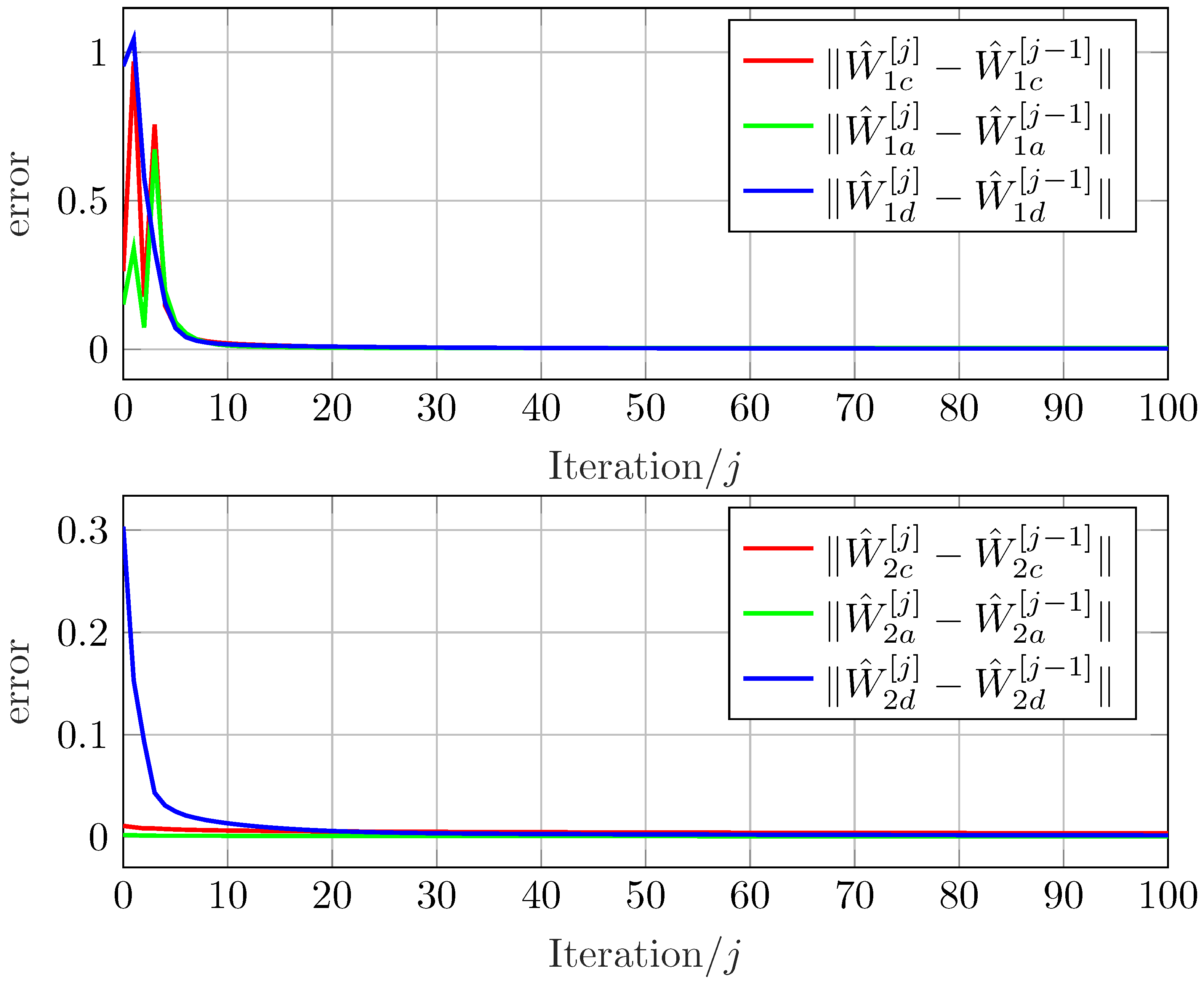
A data-driven IRL algorithm is presented to approximately achieve the Nash equilibrium strategies and the value functions without using the knowledge of the UAV dynamics. We develop an improved actor-critic-disturbance NN weights update law by using the recursive Ridge regression with the forgetting factor (${\mathrm{R}}^3{\mathrm{F}}^2$) estimator, which is more computationally efficient than the least-squares (LS) method adopted in [11,27,28,29,30,31]. The results also show that the weight parameter estimation converges exponentially to a small neighborhood of the true value.

(3)

In order to generate the learning dataset for the off-policy IRL algorithm, we introduce a novel behavior policy that is different from the conventional one used in [19,23,27,28]. Instead of using an initially admissible exploratory control law, the selected behavior policy exploits a stabilizing linear state feedback controller for the nominal position and attitude tracking error subsystems, which is generally easier to design and implement than the conventional policy

The rest of this paper is organized as follows. Section 2 introduces preliminaries on the UAV dynamics and the problem statement. The zero-sum differential games, as well as the associated HJI equations, are developed in Section 3, where the Nash equilibria of the games are discussed. In Section 4, the ${\mathrm{R}}^3{\mathrm{F}}^2$-based off-policy IRL algorithm is provided along with the convergence and stability analysis. A numerical example is presented to verify the theoretical results in Section 5. Finally, Section 6 concludes this paper.

Throughout this paper, $\mathbb{R}$, ${\mathbb{R}}^{+}$, ${\mathbb{R}}_{\ge 0}$, and ${\mathbb{N}}_{\ge 0}$ represent the sets of real numbers, positive real numbers, non-negative real numbers, and non-negative natural numbers, respectively. The superscript ⊤ indicates the transposition symbol. The notation ⊗ denotes the Kronecker product operator. For a vector $x\in {\mathbb{R}}^n$, $\parallel x\parallel :=\sqrt{x^{\top }x}$ denotes the Euclidean norm. For a matrix $A\in {\mathbb{R}}^{m\times n}$, $\parallel A\parallel$ represents the spectral norm of A. $\mathrm{vec}(A)={[a_1^{\top },a_2^{\top },\dots ,a_n^{\top }]}^{\top }\in {\mathbb{R}}^{mn\times 1}$ denotes a vector-valued representation of the matrix A with $a_i\in {\mathbb{R}}^m$ being the ith column of A. ${\lambda }_{max}(A)$ and ${\lambda }_{min}(A)$ indicate the maximum and minimum eigenvalues of the matrix A, respectively. If $A\in {\mathbb{R}}^{n\times n}$, $A>0$ or $A\ge 0$ indicates that A is a positive definite and semi-positive definite matrix, respectively. Given $A>0$, ${\parallel x\parallel }_A:=\sqrt{x^{\top }Ax}$ represents the A-weighted norm of x. The notation I indicates an identity matrix of appropriate dimensions. The notation $O_{m\times n}$ indicates an $m\times n$ zero matrix. The notation $1_m\in {\mathbb{R}}^m$ denotes an m-dimensional column vector with all components being 1.

2. Preliminaries

This section presents the UAV dynamics and the problem description for UAV robust optimal tracking control with external disturbance.

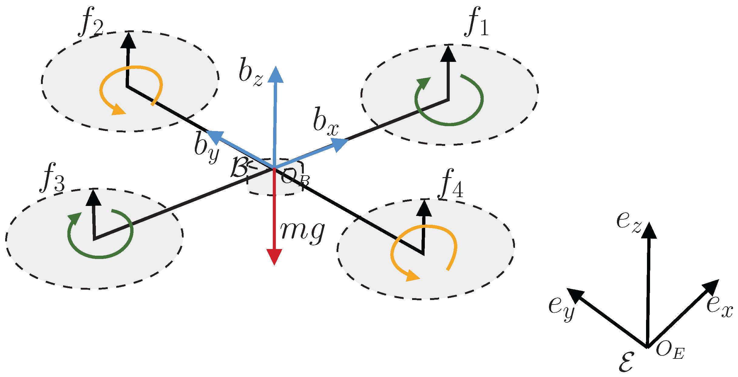
2.1. The UAV Dynamics

In this paper, the schematic diagram of a UAV is displayed in Figure 1. Let $\mathcal{E}=\{e_x,e_y,e_z\}$ be the right-handed earth-fixed inertial frame, and $\mathcal{B}=\{b_x,b_y,b_z\}$ be the body-fixed frame attached to the UAV with the origin located at its center of gravity. The thrusts of four rotors are defined as $f_i=\kappa {\omega }_i^2$, $i=1,2,3,4$, where $\kappa \in \mathbb{R}$ is a parameter and ${\omega }_i\in \mathbb{R}$ represents the ith-rotor speed. Moreover, $m\in {\mathbb{R}}^{+}$ indicates the mass of the UAV, and g is the acceleration of gravity.

The UAV dynamic modeling is based on the following assumptions to ensure theoretical tractability and practical applicability: (1) Rigid-body approximation. The UAV is modeled as a rigid body, ignoring elastic deformations and flexible components, and is validated for most fixed-wing and quadrotor systems (e.g., [32,33,34]). (2) Flat-Earth hypothesis. The Earth’s curvature and rotation are neglected; suitable for low-altitude operations (altitude $<1000$ m) ([35]). (3) Lumped aerodynamic parameters. Air resistance is described by linearized drag coefficients, with high-order effects (e.g., stall, compressibility) omitted for simplification [36]. (4) Ideal actuator dynamics. Actuators are assumed to have instantaneous responses without time delays or saturation—a condition that can be relaxed via feedback linearization in practice [37].

Denote $\zeta ={[x,y,z]}^{\top }\in {\mathbb{R}}^3$ and $\vartheta ={\left[\varphi ,\theta ,\psi \right]}^{\top }\in {\mathbb{R}}^3$ as the position and the attitude of the UAV in the $\mathcal{E}$-frame, respectively. The dynamical model takes the following form, derived from the rigid-body dynamics theory [32,33]:

$$\begin{array}{cc}\hfill & m\ddot{\zeta }=-K_{\zeta }\dot{\zeta }+R_{\mathcal{B}\mathcal{E}}{b}_{z}F-mg{b}_z+d_{\zeta }(\mathrm{translational}\mathrm{dynamics})\hfill \\ \hfill & J_b\ddot{\vartheta }=-K_{\vartheta }\dot{\vartheta }+\Lambda \tau +d_{\vartheta }(\mathrm{rotational}\mathrm{dynamics})\hfill \end{array}$$

(1)

where $F={\sum }_{i=1}^4{f}_i\in \mathbb{R}$ denotes the total thrust produced by four rotors, $\tau ={[{\tau }_{\varphi },{\tau }_{\theta },{\tau }_{\psi }]}^{\top }\in {\mathbb{R}}^3$ is the rotational torque, $b_z={[0,0,1]}^{\top }\in {\mathbb{R}}^3$, $K_{\zeta }=\mathrm{diag}(k_1,k_2,k_3)\in {\mathbb{R}}^{3\times 3}$ and $K_{\vartheta }=\mathrm{diag}(k_4,k_5,k_6)\in {\mathbb{R}}^{3\times 3}$, with $k_i\in {\mathbb{R}}^{+},i=1,\dots ,6$, denoting the aerodynamic damping coefficient matrices, and $J_b=\mathrm{diag}(I_x,I_y,I_z)\in {\mathbb{R}}^{3\times 3}$ is the inertial matrix, with $I_x,I_y,I_z\in {\mathbb{R}}^{+}$, and $d_{\zeta }={[d_x,d_y,d_z]}^{\top }\in {\mathbb{R}}^3$ and $d_{\vartheta }={[d_{\varphi },d_{\theta },d_{\psi }]}^{\top }\in {\mathbb{R}}^3$ denote the external time-varying disturbance vectors. Moreover, we have $\Lambda =\mathrm{diag}(l,l,c)\in {\mathbb{R}}^{3\times 3}$, where $l\in {\mathbb{R}}^{+}$ represents the distance from the rotor to the center of gravity, and c indicates the anti-torque coefficient. In addition, the orientation matrix $R_{\mathcal{B}\mathcal{E}}\in SO(3)$ of the UAV from the $\mathcal{B}$-frame to the $\mathcal{E}$-frame is expressed via Euler angles as follows:

$$R_{\mathcal{B}\mathcal{E}}=\left[\begin{array}{ccc}c\psi c\theta & s\varphi s\theta c\psi -c\varphi s\psi & c\varphi s\theta c\psi +s\varphi s\psi \\ c\theta s\psi & s\varphi s\theta s\psi +c\varphi c\psi & c\varphi s\theta s\psi -s\varphi c\psi \\ -s\theta & s\varphi c\theta & c\varphi c\theta \end{array}\right]$$

(2)

where $s*$ and $c*$ indicate $sin(\ast )$ and $cos(\ast )$, respectively. To avoid gimbal lock and ensure unique attitude representation, Euler angles are constrained within bounded ranges:

$$-{\displaystyle \frac{\pi }{2}}<\varphi <{\displaystyle \frac{\pi }{2}},-{\displaystyle \frac{\pi }{2}}<\theta <{\displaystyle \frac{\pi }{2}},-\pi <\psi <\pi .$$

(3)

2.2. Problem Formulation

Let ${\zeta }_r={[x_r,y_r,z_r]}^{\top }\in {\mathbb{R}}^3$ and ${\vartheta }_r={[{\varphi }_r,{\theta }_r,{\psi }_r]}^{\top }\in {\mathbb{R}}^3$ be the reference states of the position and attitude subsystems, respectively. The goal is to design F and $\tau$ such that the UAV tracks the reference states ${\zeta }_r$ and ${\vartheta }_r$ despite the presence of external time-varying disturbances $d_{\zeta }$ and $d_{\vartheta }$.

To quantify the above objective, we first define the position and attitude tracking error signals of the UAV as follows:

$${\xi }_1=\left[\begin{array}{c}\zeta -{\zeta }_r\\ \dot{\zeta }-{\dot{\zeta }}_r\end{array}\right]\in {\mathbb{R}}^6,{\xi }_2=\left[\begin{array}{c}\vartheta -{\vartheta }_r\\ \dot{\vartheta }-{\dot{\vartheta }}_r\end{array}\right]\in {\mathbb{R}}^6.$$

(4)

Substituting the derivative of (4) into (1), we can obtain the position and attitude tracking error dynamical subsystems of the UAV as follows:

$$\begin{array}{cc}\hfill {\dot{\xi }}_1& =f_1({\xi }_1)+g_{1}F+h_1{\Delta }_{\zeta },\hfill \\ \hfill {\dot{\xi }}_2& =f_2({\xi }_2)+g_2{u}_2+h_2{\Delta }_{\vartheta }\hfill \end{array}$$

(5)

where $f_1=[O_3,I_3;O_3,-{\displaystyle \frac{1}{m}}{K}_{\zeta }]·{\xi }_1\in {\mathbb{R}}^{6\times 1}$, $f_2=[O_3,I_3;O_3,-J_b^{-1}{K}_{\vartheta }]·{\xi }_2\in {\mathbb{R}}^{6\times 1}$, $g_1=[0_3;{\displaystyle \frac{1}{m}}{R}_{\mathcal{B}\mathcal{E}}{b}_z]\in {\mathbb{R}}^{6\times 1}$, $g_2=[O_3;J_b^{-1}]\in {\mathbb{R}}^{6\times 3}$, $h_1=[O_3;I_3]\in {\mathbb{R}}^{6\times 3}$, $h_2=[O_3;J_b^{-1}]\in {\mathbb{R}}^{6\times 3}$, ${\Delta }_{\zeta }=-{\displaystyle \frac{1}{m}}{K}_{\zeta }{\dot{\zeta }}_r-{\ddot{\zeta }}_r-g{b}_z+{\displaystyle \frac{1}{m}}{d}_{\zeta }\in {\mathbb{R}}^3$, ${\Delta }_{\vartheta }=-K_{\vartheta }{\dot{\vartheta }}_r-J_b{\ddot{\vartheta }}_r+d_{\vartheta }\in {\mathbb{R}}^3$, and $u_2=\Lambda \tau \triangleq {[u_{\varphi },u_{\theta },u_{\psi }]}^{\top }\in {\mathbb{R}}^3$.

Inspired by [32], we introduce a virtual position control input $u_1={[u_x,u_y,u_z]}^{\top }\in {\mathbb{R}}^3$ described by

$$\begin{array}{c}\hfill u_1=-g{b}_z+{\displaystyle \frac{1}{m}}F{R}_r{b}_z\end{array}$$

(6)

where $R_r\in {\mathbb{R}}^{3\times 3}$ is the rotational command matrix given by the following:

$$R_r=\left[\begin{array}{ccc}c{\theta }_{r}c{\psi }_r& s{\varphi }_r{s}_{{\theta }_r}c{\psi }_r-c{\varphi }_{r}s{\psi }_r& c{\varphi }_{r}s{\theta }_{r}c{\psi }_r+s{\varphi }_{r}s{\psi }_r\\ c{\theta }_{r}s{\psi }_r& s{\varphi }_{r}s{\theta }_{r}s{\psi }_r+c{\varphi }_{r}c{\psi }_r& c{\varphi }_{r}s{\theta }_{r}s{\psi }_r-s{\varphi }_{r}c{\psi }_r\\ -s{\varphi }_r& s{\varphi }_{r}c{\theta }_r& c{\varphi }_{r}c{\theta }_r\end{array}\right]$$

with ${\varphi }_r$, ${\theta }_r$, and ${\psi }_r$ being the reference states of the attitude. By solving (6), we get

$$\left\{\begin{array}{cc}F=m\parallel u_1+g{b}_z\parallel \hfill & \\ {\theta }_r=arctan({\displaystyle \frac{u_{x}c{\psi }_r+u_{y}s{\psi }_r}{u_z+g}})\hfill & \\ {\varphi }_r=arcsin({\displaystyle \frac{u_{x}s{\psi }_r-u_{y}c{\psi }_r}{\parallel u_1+g{b}_z\parallel }})\hfill \end{array}\right.$$

(7)

where ${\psi }_r$ is the reference yaw angle.

By adding and subtracting $u_1$ to ${\dot{\xi }}_1$, we can rewrite (5) in the following uniform form:

$${\dot{\xi }}_i=F_i{\xi }_i+G_i\left(u_i+v_i\right),i=1,2$$

(8)

where $u_1$ and $u_2$ are the controllers to be designed, $F_1=[O_3,I_3;O_3,-{\displaystyle \frac{1}{m}}{K}_{\zeta }]\in {\mathbb{R}}^{6\times 6}$, $G_1=[O_3;I_3]\in {\mathbb{R}}^{6\times 3}$, $F_2=[O_3,I_3;O_3,-J_b^{-1}{K}_{\vartheta }]\in {\mathbb{R}}^{6\times 6}$, and $G_2=[O_3;J_b^{-1}]\in {\mathbb{R}}^{6\times 3}$. Furthermore, $v_1=-{\displaystyle \frac{1}{m}}{K}_{\zeta }{\dot{\zeta }}_r-{\ddot{\zeta }}_r+{\displaystyle \frac{1}{m}}{d}_{\zeta }+f_{\vartheta }(F)\in {\mathbb{R}}^3$ and $v_2=-K_{\vartheta }{\dot{\vartheta }}_r-J_b{\ddot{\vartheta }}_r+d_{\vartheta }\in {\mathbb{R}}^3$ refer to the lumped disturbances acting on the position and attitude tracking error subsystems. The vector $f_{\vartheta }(F)={\displaystyle \frac{1}{m}}F(R_{\mathcal{B}\mathcal{E}}-R_r)b_z\in {\mathbb{R}}^3$ in $v_1$ is regarded as the coupling uncertainty that demonstrates the effect on the translational motion caused by rotational motion. Consequently, the control objective is cast to design $u_1$ and $u_2$ so that $\zeta (t)$ and $\psi (t)$ can track the reference signals ${\zeta }_r=[x_r,y_r,z_r]$ and ${\psi }_r$ under the time-varying disturbances $v_1$ and $v_2$.

Then, the robust tracking control problem of a UAV subject to external time-varying disturbances can be stated as follows:

Problem 1.

The purpose of the UAV robust optimal tracking control is to find an optimal state feedback control law $u_i$ such that (1) the tracking error subsystems described in (8) are closed-loop stable when $v_i=0$; (2) the bounded ${\mathcal{L}}_2$-gain condition holds when $v_i\ne 0$, that is, given ${\eta }_i>0$,

$${\int }_0^T\parallel {\xi }_i{(t)\parallel }_{{\widehat{Q}}_i}^2+\parallel u_i{(t)\parallel }_{{\widehat{R}}_i}^2\mathrm{d}t\le {\eta }_i^2{\int }_0^T{\parallel v_i(t)\parallel }^2\mathrm{d}t+\chi ({\xi }_i(0))$$

(9)

is satisfied for all $T>0$ and $v_i(t)\in {\mathcal{L}}_2[0,\infty )$, where ${\widehat{Q}}_i\in {\mathbb{R}}^{6\times 6}$, ${\widehat{R}}_i\in {\mathbb{R}}^{3\times 3}$, ${\widehat{Q}}_i={\widehat{Q}}_i^{\top }>0$, ${\widehat{R}}_i={\widehat{R}}_i^{\top }>0$, and $\chi ({\xi }_i(t))\in {\mathcal{C}}^2$ with $\chi (0)=0$.

3. Game-Based Robust Optimal Control Law Design and Stability Analysis

In this section, we formulate the robust control problem for the subsystems in (8) as two independent zero-sum differential games. Then, the Nash equilibrium is studied.

3.1. Zero-Sum Differential Games

In order to ensure robust performance under the lumped disturbances, according to inequality (9), we can define the performance index function as

$$J_i({\xi }_i(0),u_i,v_i)={\int }_0^{\infty }{q}_i({\xi }_i(t),u_i(t),v_i(t))\mathrm{d}t,i=1,2$$

(10)

where $q_i({\xi }_i(t),u_i(t),v_i(t))$ refers to an instantaneous reward function defined as $q_i({\xi }_i(t),u_i(t),v_i(t))=\parallel {\xi }_i{(t)\parallel }_{{\widehat{Q}}_i}^2+\parallel u_i{(t)\parallel }_{{\widehat{R}}_i}^2-{\eta }_i^2{\parallel v_i(t)\parallel }^2$.

In tracking error dynamics (8), the controller and the lumped disturbance can be regarded as the control player and disturbance player, respectively. Then, the robust tracking control problem can be reformulated as the following game problems with respect to (8):

Problem 2.

(Zero-sum differential games). The zero-sum differential games for the UAV robust tracking control can be represented as

$${\mathcal{G}}_i:\underset{u_i}{min}\underset{v_i}{max}{J}_i({\xi }_i(0),u_i,v_i)\mathrm{s}.\mathrm{t}.(8)$$

(11)

where ${\mathcal{G}}_1$ and ${\mathcal{G}}_2$ are the games for the position tracking control and attitude tracking control, respectively.

In game ${\mathcal{G}}_i$, $i=1,2$, the control player aims to seek the optimal control input $u_i^{*}$ that minimizes $J_i({\xi }_i(0),u_i,v_i)$, while the disturbance player desires to find the worst-case disturbance $v_i^{*}$ that maximizes it. The corresponding Nash equilibrium strategy is defined as follows:

Definition 1.

(Nash equilibrium strategy): The policy pair $(u_i^{*},v_i^{*})$ is said to be a Nash equilibrium strategy for the zero-sum differential game ${\mathcal{G}}_i$, $i=1,2$, if the inequality

$$J_i({\xi }_i(0),u_i^{*},v_i)\le J_i({\xi }_i(0),u_i^{*},v_i^{*})\le J_i({\xi }_i(0),u_i,v_i^{*})$$

(12)

holds for all $u_i$ and $v_i$. The value $J_i({\xi }_i(0),u_i^{*},v_i^{*})$ is the so-called Nash equilibrium.

In the following subsection, we will prove that the Nash equilibrium strategies are solutions to the zero-sum differential game problems ${\mathcal{G}}_i$, $i=1,2$.

3.2. Stability and Nash Equilibria for Zero-Sum Differential Games

According to the performance index defined in (10), we define the value functions for game ${\mathcal{G}}_i$, $i=1,2$, by

$$V_i({\xi }_i(t))={\int }_t^{\infty }{q}_i\left({\xi }_i(\tau ),u_i(\tau ),v_i(\tau )\right)\mathrm{d}\tau .$$

(13)

For convenience in the derivation, $i=1,2$ is omitted in the following discussion. Let the associated Hamiltonian function of (13) be defined as

$$H_i({\xi }_i,u_i,v_i,V_i,t)=\nabla V_i^{\top }\dot{{\xi }_i}(t)+q_i({\xi }_i(\tau ),u_i(\tau ),v_i(\tau ))$$

(14)

where the derivative of (10) with respect to ${\xi }_i$ is given by $\nabla V_i={\displaystyle \frac{\partial V_i}{\partial {\xi }_i}}$.

Let $V_i^{*}({\xi }_i(t))$ be the optimal value of $V_i({\xi }_i(t))$, i.e.,

$$V_i^{*}({\xi }_i(t))=\underset{u_i}{min}\underset{v_i}{max}{\int }_t^{\infty }{q}_i\left({\xi }_i(\tau ),u_i(\tau ),v_i(\tau )\right)\mathrm{d}\tau .$$

It can be easily verified that $V_i^{*}({\xi }_i(t))$ satisfies the following HJI equation:

$$\begin{array}{cc}\hfill \underset{u_i}{min}\underset{v_i}{max}{H}_i({\xi }_i,u_i,v_i,V_i,t)& =\nabla V_i^{*\top }\left[F_i{\xi }_i(t)+G_i(u_i^{*}(t)+v_i^{*}(t))\right]\hfill \\ \hfill & +\parallel {\xi }_i{(t)\parallel }_{{\widehat{Q}}_i}^2+\parallel u_i^{*}{(t)\parallel }_{{\widehat{R}}_i}^2-{\eta }_i^2{\parallel v_i^{*}(t)\parallel }^2=0\hfill \end{array}$$

(15)

where $\nabla V_i^{*}={\displaystyle \frac{\partial V_i^{*}}{\partial {\xi }_i}}$. By employing the stationary conditions ${\displaystyle \frac{\partial H_i}{\partial u_i^{*}}}=0$ and ${\displaystyle \frac{\partial H_i}{\partial v_i^{*}}}=0$, we have

$$u_i^{*}=-{\displaystyle \frac{1}{2}}{\widehat{R}}_i^{-1}{G}_i^{\top }\nabla V_i^{*},v_i^{*}={\displaystyle \frac{1}{2{\eta }_i^2}}{G}_i^{\top }\nabla V_i^{*}.$$

(16)

Substituting (16) into (15), one gets the HJI equation:

$$\begin{array}{cc}\hfill 0& =H_i({\xi }_i,u_i^{*},v_i^{*},V_i^{*},t)\hfill \\ \hfill & =\parallel {\xi }_i{(t)\parallel }_{{\widehat{Q}}_i}^2-{\displaystyle \frac{1}{4}}\nabla V_i^{*\top }{G}_i{\widehat{R}}_i^{-1}{G}_i^{\top }\nabla V_i^{*}+\nabla V_i^{*\top }{F}_i{\xi }_i(t)+{\displaystyle \frac{1}{4{\eta }_i^2}}\nabla V_i^{*\top }{G}_i{G}_i^{\top }\nabla V_i^{*}\hfill \end{array}$$

(17)

with $V_i(0)=0$.

The following theorem illustrates that (16), obtained by solving the above HJI equation in (17), provides a solution for both Problems 1 and 2:

Theorem 1.

Suppose that $0<V_i^{*}\in {\mathcal{C}}^2$ satisfies the HJI equation (17). Then, under the policy pair $(u_i^{*},v_i^{*})$ given by (16) in terms of $V_i^{*}$, the subsystems in (8) are closed-loop stable and the bounded ${\mathcal{L}}_2$-gain condition (9) holds. Moreover, $(u_i^{*},v_i^{*})$ is a Nash equilibrium strategy of ${\mathcal{G}}_i$, $i=1,2$.

Proof. 

Suppose that $V_i^{*}$ satisfies HJI equation (17). Then,

$$\begin{array}{cc}\hfill & H_i({\xi }_i,u_i,v_i,V_i^{*},t)-H_i({\xi }_i,u_i^{*},v_i^{*},V_i^{*},t)\hfill \\ \hfill & =\nabla V_i^{*\top }{G}_i(u_i(t)-u_i^{*}(t))+\parallel u_i{(t)\parallel }_{{\widehat{R}}_i}^2-{\parallel u_i^{*}(t)\parallel }_{{\widehat{R}}_i}^2\hfill \\ \hfill & +\nabla V_i^{*\top }{G}_i(v_i(t)-v_i^{*}(t))-{\eta }_i^2(\parallel v_i{(t)\parallel }^2-\parallel v_i^{*}(t){\parallel }^2).\hfill \end{array}$$

(18)

According to the Hamiltonian function (14), the following identity holds:

$$\begin{array}{cc}\hfill {\dot{V}}_i^{*}({\xi }_i(t))=& H_i({\xi }_i,u_i^{*},v_i^{*},V_i^{*},t)+{\parallel u_i(t)-u_i^{*}(t)\parallel }_{{\widehat{R}}_i}^2\hfill \\ \hfill & -q_i\left({\xi }_i(t),u_i(t),v_i(t)\right)-{\eta }_i^2{\parallel v_i(t)-v_i^{*}(t)\parallel }^2.\hfill \end{array}$$

(19)

By setting $u_i(t)=u_i^{*}(t)$ and $v_i(t)=v_i^{*}(t)$ (the optimal control and disturbance strategies) and substituting them into (19), we have the following:

$${\dot{V}}_i^{*}({\xi }_i(t))=-q_i\left({\xi }_i(t),u_i^{*}(t),v_i^{*}(t)\right)\le 0,$$

(20)

where the equality ${\dot{V}}_i^{*}({\xi }_i(t))=0$ holds if and only if ${\xi }_i(t)=0$. Thus, the subsystems described in (8) are asymptotically stable.

According to the Lyapunov stability theory, since ${\dot{V}}_i^{*}({\xi }_i(t))$ is negative semidefinite and vanishes only at the origin, the subsystems described by (8) are proven to be asymptotically stable. The Lyapunov function $V_i^{*}({\xi }_i)$ satisfies the standard stability criteria, ensuring that trajectories converge to the equilibrium point ${\xi }_i(t)=0$ as $t\to \infty$.

Integrating (20) from 0 to T yields

$$\begin{array}{c}\hfill V_i^{*}({\xi }_i(T))-V_i^{*}({\xi }_i(0))=-{\int }_0^T{q}_i\left({\xi }_i(t),u_i^{*}(t),v_i^{*}(t)\right)\mathrm{d}t\le 0\end{array}$$

(21)

Since $V_i^{*}>0$, one has

$$\begin{array}{c}\hfill {\int }_0^T\parallel {\xi }_i{(t)\parallel }_{{\widehat{Q}}_i}^2+\parallel u_i^{*}{(t)\parallel }_{{\widehat{R}}_i}^2\mathrm{d}t\le V_i^{*}({\xi }_i(0))+{\eta }_i^2{\int }_0^T{\parallel v_i^{*}(t)\parallel }^2\mathrm{d}t\end{array}$$

(22)

which shows that the bounded ${\mathcal{L}}_2$-gain condition holds. Furthermore, due to the fact that the tracking subsystem is asymptotically stable, it can be concluded that $V_i^{*}({\xi }_i(\infty ))=0$. Thus, by (14), we have

$$\begin{array}{cc}\hfill J_i({\xi }_i(0),u_i,v_i)=& V_i^{*}({\xi }_i(0))+{\int }_0^{\infty }{H}_i({\xi }_i,u_i^{*},v_i^{*},V_i^{*},t)\mathrm{d}t\hfill \\ \hfill & +{\int }_0^{\infty }\left[\parallel u_i(t)-u_i^{*}{(t)\parallel }_{{\widehat{R}}_i}^2-{\eta }_i^2{\parallel v_i(t)-v_i^{*}(t)\parallel }^2\right]\mathrm{d}t.\hfill \end{array}$$

(23)

It follows that the condition (12) is satisfied. By setting $u_i=u_i^{*}$ and $v_i=v_i^{*}$, one gets $J_i({\xi }_i(0),u_i^{*},v_i^{*})=V_i^{*}({\xi }_i(0))$. Thus, $u_i^{*}$ and $v_i^{*}$ form a Nash equilibrium strategy and $V_i^{*}({\xi }_i(0))$ is the corresponding Nash equilibrium of the game ${\mathcal{G}}_i$.    □

However, as a nonlinear partial differential equation (PDE), the HJI equation given in (17) is difficult to solve directly and analytically [38]. To this end, a data-driven IRL approach is designed to obtain the solution to the HJI equation and the Nash equilibrium strategies.

4. ${\mathbf{R}}^{\mathbf{3}}{\mathbf{F}}^{\mathbf{2}}$-Based IRL Approach

In this section, an ${\mathrm{R}}^3{\mathrm{F}}^2$-based IRL algorithm is developed to solve the zero-sum differential games. First, the actor-critic-disturbance architecture is utilized to approximate the value function and the Nash equilibrium strategy. Based on this, a model-free integral Bellman equation is derived. Then, an ${\mathrm{R}}^3{\mathrm{F}}^2$-based IRL algorithm is provided to evaluate the value function and learn the Nash equilibrium strategy. Finally, the convergence and stability analysis are presented.

4.1. A Framework of $R^3{F}^2$-Based IRL for Zero-Sum Differential Games

Denote $V_i^j({\xi }_i(t))$ as the updated value function in the jth iteration, and ${\widehat{u}}_i^j$ and ${\widehat{v}}_i^j$ as the updated control policy and disturbance in the jth iteration, respectively. For all $t>0$ and $\Delta t>0$, and using the Fundamental Theorem of Calculus and the definition of the performance index (13), the increment of the value function $V_i^j({\xi }_i)$ over the interval $[t,t+\Delta t]$ is as follows:

$$\begin{array}{cc}\hfill V_i^j({\xi }_i(t+\Delta t))-V_i^j({\xi }_i(t))& ={\int }_t^{t+\Delta t}{\displaystyle \frac{d}{d\tau }}{V}_i^j({\xi }_i(\tau ))d\tau \hfill \\ \hfill & ={\int }_t^{t+\Delta t}\nabla V_i^{j\top }({\xi }_i(\tau ))·{\dot{\xi }}_i(\tau )d\tau ,\hfill \end{array}$$

(24)

where the second equality follows from the chain rule. Rearranging this expression yields the following:

$$V_i^j({\xi }_i(\tau )){|}_t^{t+\Delta t}=-{\int }_t^{t+\Delta t}\nabla V_i^{j\top }{\dot{\xi }}_i(\tau )d\tau .$$

(25)

Define ${\tilde{u}}_i^j=u_i-{\widehat{u}}_i^j$ and ${\tilde{v}}_i^j=v_i-{\widehat{v}}_i^j$ as the estimation errors of control and disturbance, respectively. Substituting $u_i={\widehat{u}}_i^j+{\tilde{u}}_i^j$ and $v_i={\widehat{v}}_i^j+{\tilde{v}}_i^j$ into the system dynamics (8) gives the following:

$$\begin{array}{cc}\hfill {\dot{\xi }}_i& =F_i{\xi }_i+G_i\left(u_i+v_i\right)\hfill \\ \hfill & =F_i{\xi }_i+G_i\left({\widehat{u}}_i^j+{\widehat{v}}_i^j+{\tilde{u}}_i^j+{\tilde{v}}_i^j\right),\hfill \end{array}$$

(26)

where ${\widehat{u}}_i^j$ and ${\widehat{v}}_i^j$ denote the control and disturbance policies at the j-th iteration, and ${\tilde{u}}_i^{j}and{\tilde{v}}_i^j$ represent the residual errors. This decomposition separates nominal control/disturbance (${\widehat{u}}_i^j,{\widehat{v}}_i^j$) from their errors, facilitating stability analysis.

From the Hamiltonian function (14) and the optimality conditions ${\displaystyle \frac{\partial H_i}{\partial u_i}}=0$ and ${\displaystyle \frac{\partial H_i}{\partial v_i}}=0$, we can obtain

$${\widehat{u}}_i^{j+1}=-{\displaystyle \frac{1}{2}}{\widehat{R}}_i^{-1}{G}_i^{\top }\nabla V_i^j,{\widehat{v}}_i^{j+1}={\displaystyle \frac{1}{2{\eta }_i^2}}{G}_i^{\top }\nabla V_i^j,$$

(27)

where ${\widehat{R}}_i\succ 0$ and ${\eta }_i>0$ are design parameters. These satisfy the saddle-point condition ${\displaystyle \frac{{\partial }^2{H}_i}{\partial u_i^2}}\succ 0$ and ${\displaystyle \frac{{\partial }^2{H}_i}{\partial v_i^2}}\prec 0$, ensuring local optimality.

Substituting (26) and (27) into (24) yields the following model-free integral Bellman equation:

$$\begin{array}{cc}\hfill V_i^j({\xi }_i(t))-V_i^j({\xi }_i(t+\Delta t))& =-{\int }_t^{t+\Delta t}\nabla V_i^{j\top }\left[F_i{\xi }_i+G_i\left({\widehat{u}}_i^j+{\widehat{v}}_i^j+{\tilde{u}}_i^j+{\tilde{v}}_i^j\right)\right]d\tau \hfill \\ \hfill & =-{\int }_t^{t+\Delta t}\nabla V_i^{j\top }\left[F_i{\xi }_i+G_i\left({\widehat{u}}_i^j+{\widehat{v}}_i^j\right)\right]d\tau \hfill \\ \hfill & -{\int }_t^{t+\Delta t}\left[\nabla V_i^{j\top }{G}_i\left(u_i-{\widehat{u}}_i^j\right)+\nabla V_i^{j\top }{G}_i\left(v_i-{\widehat{v}}_i^j\right)\right]d\tau \hfill \\ \hfill & ={\int }_t^{t+\Delta t}\left({\xi }_i^{\top }{\widehat{Q}}_i{\xi }_i+{\widehat{u}}_i^{j\top }{\widehat{R}}_i{\widehat{u}}_i^j-{\eta }_i^2{\widehat{v}}_i^{j\top }{\widehat{v}}_i^j\right)d\tau \hfill \\ \hfill & +{\int }_t^{t+\Delta t}\left[2{\widehat{u}}_i^{j+1\top }{\widehat{R}}_i\left(u_i-{\widehat{u}}_i^j\right)-2{\eta }_i^2{\widehat{v}}_i^{j+1\top }\left(v_i-{\widehat{v}}_i^j\right)\right]d\tau \hfill \\ \hfill & ={\int }_t^{t+\Delta t}\parallel {\xi }_i{(t)\parallel }_{{\widehat{Q}}_i}^2+\parallel {\widehat{u}}_i{(t)\parallel }_{{\widehat{R}}_i}^2-{\eta }_i^2{\parallel {\widehat{v}}_i(t)\parallel }^2\mathrm{d}\tau \hfill \\ \hfill & +2{\int }_t^{t+\Delta t}{\widehat{u}}_i^{j+1\top }(\tau ){\widehat{R}}_i{\tilde{u}}_i^j(\tau )-{\eta }_i^2{\widehat{v}}_i^{j+1\top }(\tau ){\tilde{v}}_i^j(\tau )\mathrm{d}\tau .\hfill \end{array}$$

(28)

This equation holds for any $\Delta t>0$ and is model-free because it does not explicitly depend on $F_i$ or $G_i$, relying only on measurable signals ${\xi }_i$, ${\widehat{u}}_i$, and ${\widehat{v}}_i$.

Starting from an initially stabilizing control policy, the proposed algorithm first computes $V_i^j({\xi }_i(t))$ by solving the partial differential Equation (14), followed by computing $u_i^{j+1}$ and $v_i^{j+1}$ by using (27). Repeat the above-mentioned processes until the difference between $V_i^j({\xi }_i(t))$ and $V_i^{j-1}({\xi }_i(t))$ is sufficiently small.

Based on the Stone–Weierstrass approximation theorem [39], the jth iterative approximate expressions of $V_i({\xi }_i)$, $u_i$, and $v_i$ can be represented by

$${\wp }_i^j=W_i^{j\top }{\mathrm{\Phi }}_i({\xi }_i)+{ϵ}_i^j$$

(29)

where ${\wp }_i^j={[V_i^j({\xi }_i),u_i^{j+1\top },v_i^{j+1\top }]}^{\top }\in {\mathbb{R}}^7$, ${\mathrm{\Phi }}_i({\xi }_i)\in {\mathbb{R}}^{(n_i+3m_i+3l_i)\times 7}$ is a block matrix given by

$${\mathrm{\Phi }}_i({\xi }_i)\triangleq \left[\begin{array}{ccc}{\phi }_{ic}({\xi }_i)& O_{n_i\times 3}& O_{n_i\times 3}\\ O_{3m_i\times 1}& I_3\otimes {\phi }_{ia}({\xi }_i)& O_{3m_i\times 3}\\ O_{3l_i\times 1}& O_{3l_i\times 3}& I_3\otimes {\phi }_{id}({\xi }_i)\end{array}\right]$$

and ${ϵ}_i^j\in {\mathbb{R}}^7$ is the approximation error vector. In ${\mathrm{\Phi }}_i({\xi }_i)$, the components ${\phi }_{ic}({\xi }_i)\in {\mathbb{R}}^{n_i}$, ${\phi }_{ia}({\xi }_i)\in {\mathbb{R}}^{m_i}$, and ${\phi }_{id}({\xi }_i)\in {\mathbb{R}}^{l_i}$ are all activation functions, $W_i^j\in {\mathbb{R}}^{n_i+3m_i+3l_i}$ represents the weight coefficient vector in the form of $W_i^j={[W_{ic}^{j\top },vec{(W_{ia}^{j+1})}^{\top },vec{(W_{id}^{j+1})}^{\top }]}^{\top }$, with $W_{ic}^j\in {\mathbb{R}}^{n_i}$ being the weight vector of the critic NNs, and $W_{ia}^{j+1}\in {\mathbb{R}}^{m_i\times 3}$ and $W_{id}^{j+1}\in {\mathbb{R}}^{l_i\times 3}$ being weight matrices of the actor NNs and lumped disturbance NNs, respectively. Note that $W_i^j$ is unknown and, thus, needs to be estimated. Denote ${\widehat{W}}_{ic}^j$, ${\widehat{W}}_{ia}^{j+1}$, and ${\widehat{W}}_{id}^{j+1}$ as the estimated values of $W_{ic}^j$, $W_{ia}^{j+1}$, and $W_{id}^{j+1}$, respectively. The estimate of ${\wp }_i^j$ is given by

$${\widehat{\wp }}_i^j={\mathrm{\Phi }}_i^{\top }({\xi }_i){\widehat{W}}_i^j$$

(30)

where ${\widehat{W}}_i^j={\left[{\widehat{W}}_{ic}^{j\top },vec{({\widehat{W}}_{ia}^{j+1})}^{\top },vec{({\widehat{W}}_{id}^{j+1})}^{\top }\right]}^{\top }$.

Assumption 1.

(1) 

The activation functions of actor-critic-disturbance NNs and their derivatives are bounded, i.e., $\parallel {\phi }_{ia}\parallel \le b_{{\phi }_{ia}}$, $\parallel {\phi }_{ic}\parallel \le b_{{\phi }_{ic}}$, $\parallel {\phi }_{id}\parallel \le b_{{\phi }_{id}}$, $\parallel \nabla {\phi }_{ia}\parallel \le b_{d{\phi }_{ia}}$, $\parallel \nabla {\phi }_{ic}\parallel \le b_{d{\phi }_{ic}}$, and $\parallel \nabla {\phi }_{id}\parallel \le b_{d{\phi }_{id}}$, where $b_{{\phi }_{ia}}$, $b_{{\phi }_{ic}}$, $b_{{\phi }_{id}}$, $b_{d{\phi }_{ia}}$, $b_{d{\phi }_{ic}}$, and $b_{d{\phi }_{id}}$ are positive constants.

(2) 

The ideal actor-critic-disturbance NN weights satisfy $\parallel W_{ic}^j\parallel \le W_{icmax}^j$, $\parallel W_{ia}^{j+1}\parallel \le W_{iamax}^{j+1}$, and $\parallel W_{id}^{j+1}\parallel \le W_{idmax}^{j+1}$, where $W_{icmax}^j$, $W_{iamax}^{j+1}$ and $W_{idmax}^{j+1}$ are positive constants.

(3) 

$\parallel {ϵ}_i^j\parallel \le b_{{ϵ}_i^j}$ and $\parallel \nabla {ϵ}_i^j\parallel \le b_{d{ϵ}_i^j}$, where $b_{{ϵ}_i^j}$ and $b_{d{ϵ}_i^j}$ are positive constants.

Let $\Delta {\phi }_{ic}\triangleq \Delta {\phi }_{ic}({\xi }_i(t))={\phi }_{ic}({\xi }_i(t+\Delta t))-{\phi }_{ic}({\xi }_i(t))$. According to (28) and (30), one has

$$\begin{array}{cc}\hfill 0=& V_i^j({\xi }_i(t+\Delta t))-V_i^j({\xi }_i(t))+{\int }_t^{t+\Delta t}\parallel {\xi }_i{(t)\parallel }_{{\widehat{Q}}_i}^2+\parallel {\widehat{u}}_i{(t)\parallel }_{{\widehat{R}}_i}^2-{\eta }_i^2{\parallel {\widehat{v}}_i(t)\parallel }^2\mathrm{d}\tau \hfill \\ \hfill & +2{\int }_t^{t+\Delta t}{\widehat{u}}_i^{j+1\top }(\tau ){\widehat{R}}_i{\tilde{u}}_i^j(\tau )-{\eta }_i^2{\widehat{v}}_i^{j+1\top }(\tau ){\tilde{v}}_i^j(\tau )\mathrm{d}\tau \hfill \\ \hfill =& \Delta {\phi }_{ic}^{\top }({\xi }_i(t)){\widehat{W}}_{ic}^j+{\int }_t^{t+\Delta t}{q}_i({\xi }_i(\tau ),{\widehat{u}}_i(\tau ),{\widehat{v}}_i(\tau ))\mathrm{d}\tau \hfill \\ \hfill & +2{\int }_t^{t+\Delta t}{\widehat{u}}_i^{j+1\top }(\tau ){\widehat{R}}_i{\tilde{u}}_i^j(\tau )-{\eta }_i^2{\widehat{v}}_i^{j+1\top }(\tau ){\tilde{v}}_i^j(\tau )\mathrm{d}\tau .\hfill \end{array}$$

(31)

By using (27) we can obtain the following:

$$\begin{array}{cc}\hfill & {\widehat{u}}_i^{j+1\top }(\tau ){\widehat{R}}_i{\tilde{u}}_i^j(\tau )=[({\tilde{u}}_i^{j\top }(\tau ){\widehat{R}}_i)\otimes {\phi }_{ia}^{\top }({\xi }_i(\tau ))]vec({\widehat{W}}_{ia}^{j+1}),\hfill \\ \hfill & {\widehat{v}}_i^{j+1\top }(\tau ){\tilde{v}}_i^j(\tau )=[{\tilde{v}}_i^{j\top }(\tau )\otimes {\phi }_{id}^{\top }({\xi }_i(\tau ))]vec({\widehat{W}}_{id}^{j+1}).\hfill \end{array}$$

(32)

Substituting (32) into (31) yields

$$\begin{array}{c}\hfill C_{i\xi }^j(t)={\mathrm{\Xi }}_i^{j\top }(t){\widehat{W}}_i^j\end{array}$$

(33)

where ${\widehat{W}}_i^j={[{\widehat{W}}_{ic}^{j\top },vec{({\widehat{W}}_{ia}^{j+1})}^{\top },vec{({\widehat{W}}_{id}^{j+1})}^{\top }]}^{\top }\in {\mathbb{R}}^{n_i+3m_i+3l_i}$, ${\mathrm{\Xi }}_i^j(t)\in {\mathbb{R}}^{n_i+3m_i+3l_i}$ and $C_{i\xi }^j(t)\in \mathbb{R}$ are respectively expressed by

$$\begin{array}{cc}\hfill & {\mathrm{\Xi }}_i^j(t)={\left[C_{ic}^j(t),C_{ia}^j(t),C_{id}^j(t)\right]}^{\top },\hfill \\ \hfill & C_{i\xi }^j(t)=-{\int }_t^{t+\Delta t}{q}_i({\xi }_i(\tau ),{\widehat{u}}_i(\tau ),{\widehat{v}}_i(\tau ))\mathrm{d}\tau .\hfill \end{array}$$

(34)

In (34), $C_{ic}^j(t)=\Delta {\phi }_{ic}^{\top }({\xi }_i(t))\in {\mathbb{R}}^{1\times n_i}$, $C_{ia}^j(t)\in {\mathbb{R}}^{1\times 3m_i}$, and $C_{id}^j(t)\in {\mathbb{R}}^{1\times 3l_i}$, are respectively defined as

$$\begin{array}{cc}\hfill & C_{ia}^j(t)=2{\int }_t^{t+\Delta t}({\tilde{u}}_i^{j\top }(\tau ){\widehat{R}}_i)\otimes {\phi }_{ia}^{\top }({\xi }_i(\tau ))\mathrm{d}\tau ,\hfill \\ \hfill & C_{id}^j(t)=-2{\eta }_i^2{\int }_t^{t+\Delta t}{\tilde{v}}_i^{j\top }(\tau )\otimes {\phi }_{id}^{\top }({\xi }_i(\tau ))\mathrm{d}\tau .\hfill \end{array}$$

Note that (33) is a linear equation, where $C_{i\xi }^j(t)$ denotes the measurements, ${\mathrm{\Xi }}_i^j(t)$ is the regression matrix, respectively, at time t, and ${\widehat{W}}_i^j$ is the uncertain vector to be estimated. The value of $C_{i\xi }^j(t)$ and the data in ${\mathrm{\Xi }}_i^j(t)$ are typically obtained from a continuous-time process and are available at the sample times $k\Delta t$, where $\Delta t$ is the sample interval. To compute the estimate of ${\widehat{W}}_i^j$, we first construct two datasets, ${\mathcal{C}}_i^j=\{C_{i\xi |0}^j,C_{i\xi |1}^j,\dots ,C_{i\xi |k}^j\}$ and ${\mathcal{E}}_i^j=\{{\mathrm{\Xi }}_{i|0}^j,{\mathrm{\Xi }}_{i|1}^j,\dots ,{\mathrm{\Xi }}_{i|k}^j\}$, by utilizing the data produced by the behavior policy over the time window $\ell =0,1,\dots ,k$.

Then, we can use the ${\mathrm{R}}^3{\mathrm{F}}^2$ scheme to find the optimal estimate ${\widehat{W}}_{i|k}^j$ of ${\widehat{W}}_i^j$ by solving the following optimization problem:

Problem 3.

$$\begin{array}{cc}\hfill & \underset{{\widehat{W}}_i^j}{min}{\mathcal{Y}}_{ik}({\widehat{W}}_i^j)={\displaystyle \frac{1}{2}}{\rho }_i^k{\parallel {\widehat{W}}_i^j-{\widehat{W}}_{i|0}^j\parallel }_{P_{i0}^{-j}}^2+{\displaystyle \frac{1}{2}}\sum _{\ell =0}^k{\rho }_i^{k-\ell }{\varsigma }_{i|\ell }^{j2}\hfill \\ \hfill & \mathrm{s}.\mathrm{t}.{\varsigma }_{i|\ell }^j=C_{i\xi |\ell }^j-{\mathrm{\Xi }}_{i|\ell }^{j\top }{\widehat{W}}_i^j,\ell =0,1,\dots ,k\hfill \end{array}$$

where ${\rho }_i\in (0,1]$ represents the forgetting factor, ${\widehat{W}}_{i|0}^j\in {\mathbb{R}}^{n_i+3m_i+3l_i}$ indicates the initial estimate of ${\widehat{W}}_i^j$, $P_{i0}^j\in {\mathbb{R}}^{(n_i+3m_i+3l_i)\times (n_i+3m_i+3l_i)}$ is positive definite, and $P_{i0}^{-j}$ denotes the inverse matrix, ${(P_{i0}^j)}^{-1}$, of $P_{i0}^j$ for brevity.

Remark 1.

In most of the existing works (e.g., [27,28,40]), the LS scheme is applied to approximate the solution to (33), in which random or sinusoidal function noises are usually added to the behavior policy to ensure that the matrix $\left[{\mathrm{\Xi }}_{i|0}^j,{\mathrm{\Xi }}_{i|1}^j,\dots ,{\mathrm{\Xi }}_{i|k}^j\right]$ has full column rank. However, the selection of rich input signals is usually experience-based. In Problem 3, the exponentially weighted mechanism is used to apply greater weights to the recent data, and the weighted vector norm regularization term ${\displaystyle \frac{1}{2}}{\rho }_i^k{\parallel {\widehat{W}}_i^j-{\widehat{W}}_{i|0}^j\parallel }_{P_{i0}^{-j}}^2$ is designed to address the numerical instability of the matrix inversion and subsequently produce lower variance models.

We can obtain the optimal solution to Problem 3 as

$${\widehat{W}}_{i|k}^j=P_{i|k}^j{S}_{i|k}^j$$

where $P_{i|k}^j$ and $S_{i|k}$ are given by

$$\begin{array}{cc}\hfill P_{i|k}^j& ={\left(\sum _{\ell =0}^k{\rho }_i^{k-\ell }{\mathrm{\Xi }}_{i|\ell }^j{\mathrm{\Xi }}_{i|\ell }^{j\top }+{\rho }_i^k{P}_{i0}^{-j}\right)}^{-1},\hfill \\ \hfill S_{i|k}^j& =\sum _{\ell =0}^k{\rho }_i^{k-\ell }{C}_{i\xi |\ell }^j{\mathrm{\Xi }}_{i|\ell }^j+{\rho }_i^k{P}_{i0}^{-j}{\widehat{W}}_{i|0}^j.\hfill \end{array}$$

(35)

Then, for all $k\in {\mathbb{N}}_{\ge 0}$, we can obtain the update rule for ${\widehat{W}}_{i|k}^j$ as follows:

$${\widehat{W}}_{i|k}^j={\widehat{W}}_{i|(k-1)}^j+P_{i|k}^j{\mathrm{\Xi }}_{i|k}^j{\overline{\varsigma }}_{i|k}$$

(36)

where

$$\begin{array}{cc}\hfill & {\overline{\varsigma }}_{i|k}=C_{i\xi |k}^j-{\mathrm{\Xi }}_{i|k}^{j\top }{\widehat{W}}_{i|(k-1)}^j\hfill \\ \hfill & P_{i|k}^j={\rho }_i^{-1}(P_{i|(k-1)}^j-{\sigma }_{i|k}^{-j}\parallel P_{i|(k-1)}^j{\mathrm{\Xi }}_{i|k}^j{\parallel }^2)\hfill \end{array}$$

(37)

with ${\sigma }_{i|k}^j={\rho }_i+{\mathrm{\Xi }}_{i|k}^{j\top }{P}_{i|(k-1)}^j{\mathrm{\Xi }}_{i|k}^j.$

Remark 2.

The computational requirements of $R^3{F}^2$ are primarily determined by $n_i+3m_i+3l_i$. Since $P_{i|k}^j$ is of size $(n_i+3m_i+3l_i)\times (n_i+3m_i+3l_i)$, the computational requirement for updating $P_{i|k}^j$ given by (37) is of $O({(n_i+3m_i+3l_i)}^2)$. Moreover, the ${\sigma }_{i|k}^{-j}$ in (37) is of $O(1)$, which is much less demanding than the matrix inverse operation required by the LS algorithm. In addition, the storage requirements of the recursive $R^3{F}^2$ are of $O({(n_i+3m_i+3l_i)}^2)$, which does not grow with k. Thus, the computational and memory requirements of the recursive $R^3{F}^2$ are significantly less than those of LS.

The implementation procedure of the proposed ${\mathrm{R}}^3{\mathrm{F}}^2$-based IRL approach is summarized in Algorithm 1. For a fixed controller $u_i$ and the arbitrary uncertainty signals $v_i$, the proposed algorithm can simultaneously learn estimates of the value function $V_i^j({\xi }_i)$, control policy $u_i^{j+1}$, and uncertainties $v_i^{j+1}$ without applying the knowledge of the UAV dynamics.

Algorithm 1: ${\mathrm{R}}^3{\mathrm{F}}^2$-based IRL for zero-sum differential games

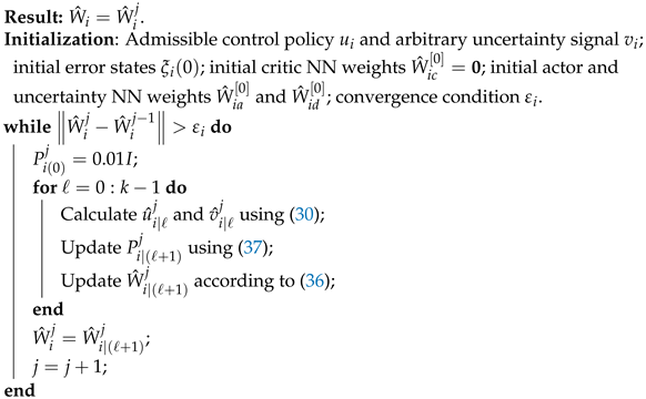
4.2. Convergence and Stability Analysis

The following results show that the NN weight tuning laws guarantee the proposed ${\mathrm{R}}^3{\mathrm{F}}^2$-based IRL algorithm converges to the Nash equilibrium strategy, while ensuring the stability of the closed-loop system.

Define ${\tilde{\widehat{W}}}_{i|k}^j={\widehat{W}}_i^j-{\widehat{W}}_{i|k}^j$ and ${\tilde{W}}_{i|k}^j=W_i^j-{\widehat{W}}_{i|k}^j$.

Then, it follows from (36) that ${\tilde{\widehat{W}}}_{i|k}^j$ and ${\tilde{W}}_{i|k}^j$ can be written as

$$\begin{array}{cc}\hfill & {\tilde{\widehat{W}}}_{i|k}^j=(I-P_{i|k}^j{\mathrm{\Xi }}_{i|k}^j{\mathrm{\Xi }}_{i|k}^{j\top }){\tilde{\widehat{W}}}_{i|k-1}^j,\hfill \end{array}$$

(38a)

$$\begin{array}{cc}\hfill & {\tilde{W}}_{i|k}^j={\tilde{W}}_{i|(k-1)}^j-P_{i|k}^j{\mathrm{\Xi }}_{i|k}^j{\mathrm{\Xi }}_{i|k}^{j\top }{\tilde{\widehat{W}}}_{i|(k-1)}^j.\hfill \end{array}$$

(38b)

Definition 2.

The matrix sequence, ${\left\{{\mathrm{\Xi }}_{i|k}^j\right\}}_{k=0}^{\infty }$, is said to be persistently exciting (PE) if for some $N\in {\mathbb{N}}_{\ge 0}$ and $\forall \ell \in {\mathbb{N}}_{\ge 0}$, $\exists {\beta }_1,{\beta }_2\in {\mathbb{R}}^{+}$ such that ${\beta }_{1}I\le {\sum }_{l=\ell }^{\ell +N}{\mathrm{\Xi }}_{i|l}^j{\mathrm{\Xi }}_{i|l}^{j\top }\le {\beta }_{2}I<\infty$.

Lemma 1.

Suppose that ${\left\{{\mathrm{\Xi }}_{i|k}^j\right\}}_{k=0}^{\infty }$ is PE. Let $N,{\beta }_1$ and ${\beta }_2$ be given by Definition 2, ${\rho }_i\in (0,1]$, and $P_{i|k}^j$ be given by (37). Then, for all $k\ge N+1$,

$$0<{\overline{\beta }}_{1}I\le P_{i|k}^{-j}\le {\overline{\beta }}_{2}I+P_N^{-1}<\infty$$

(39)

with ${\overline{\beta }}_1={\displaystyle \frac{{\rho }_i^N(1-{\rho }_i)}{1-{\rho }_i^{N+1}}}{\beta }_1$ and ${\overline{\beta }}_2={\displaystyle \frac{1}{1-{\rho }_i^{N+1}}}{\beta }_2$.

Theorem 2

(Convergence of ${\mathrm{R}}^3{\mathrm{F}}^2$-Based IRL Algorithm). Let (36) be the update rule of the actor-critic-disturbance NN weights. Suppose that ${\left\{{\mathrm{\Xi }}_{i|k}^j\right\}}_{k=0}^{\infty }$ is PE. Then, for any initial condition ${\widehat{W}}_{i|0}^j$, the estimation error ${\tilde{\widehat{W}}}_{i|k}^j$ converges exponentially to the origin, i.e., for any ${\widehat{W}}_{i|0}^j$ there exists ${\gamma }_0\in {\mathbb{R}}^{+}$ such that for all $k\in {\mathbb{N}}_{\ge 0}$,

$$\parallel {\tilde{\widehat{W}}}_{i|k}^j{\parallel }^2\le {\gamma }_0{\rho }_i^k{\parallel W_{i|0}^j\parallel }^2$$

(40)

and ${\tilde{W}}_{i|k}^j$ is ultimately uniformly bounded (UUB).

Proof. 

Define the Lyapunov function candidate as

$${\widehat{\mathcal{L}}}_{i|k}^j={\tilde{\widehat{W}}}_{i|k}^{j\top }{P}_{i|k}^{-j}{\tilde{\widehat{W}}}_{i|k}^j.$$

(41)

Since

$$P_{i|k}^{-j}={\rho }_i{P}_{i|(k-1)}^{-j}+{\mathrm{\Xi }}_{i|k}^j{\mathrm{\Xi }}_{i|k}^{j\top },$$

(42)

using (42) and (38a), one has

$$\begin{array}{cc}\hfill \Delta {\widehat{\mathcal{L}}}_{i|k}^j& =:{\widehat{\mathcal{L}}}_{i|k}^j-{\widehat{\mathcal{L}}}_{i|(k-1)}^j\hfill \\ \hfill & =-{\tilde{\widehat{W}}}_{i|k-1}^{j\top }{\mathrm{\Xi }}_{i|k}^j\left(1-{\mathrm{\Xi }}_{i|k}^{j\top }{P}_{i|k}^j{\mathrm{\Xi }}_{i|k}^j\right){\mathrm{\Xi }}_{i|k}^{j\top }{\tilde{\widehat{W}}}_{i|(k-1)}^j+({\rho }_i-1){\tilde{\widehat{W}}}_{i|k-1}^{j\top }{P}_{i|(k-1)}^{-j}{\tilde{\widehat{W}}}_{i|(k-1)}^j.\hfill \end{array}$$

(43)

Moreover, it follows from (42) and ${\rho }_i\in (0,1]$ that

$$P_{i|k}^{-j}\ge {\rho }_i{P}_{i|(k-1)}^{-j}\ge \dots \ge {\rho }_i^k{P}_{i|0}^{-j}>0.$$

(44)

Thus, for all $k\in {\mathbb{N}}_{\ge 0}$, ${\widehat{\mathcal{L}}}_{i|k}^j\ge {\lambda }_{min}(P_{i|0}^{-j}){\rho }_i^k{\parallel {\tilde{\widehat{W}}}_{i|k}^j\parallel }^2$.

Denote $a={\mathrm{\Xi }}_{i|k}^{j\top }{P}_{i|(k-1)}^j{\mathrm{\Xi }}_{i|k}^j>0$. Using (37), we can obtain

$$\begin{array}{c}\hfill 1-{\mathrm{\Xi }}_{i|k}^{j\top }{P}_{i|k}^j{\mathrm{\Xi }}_{i|k}^j={\displaystyle \frac{{\rho }_i}{{\rho }_i+a}}>0.\end{array}$$

(45)

Combining (45) with (43) leads to

$$\begin{array}{c}\hfill {\widehat{\mathcal{L}}}_{i|k}^j-{\widehat{\mathcal{L}}}_{i|(k-1)}^j\le ({\rho }_i-1){\widehat{\mathcal{L}}}_{i|(k-1)}^j\le 0\end{array}$$

(46)

which in turn gives

$${\widehat{\mathcal{L}}}_{i|k}^j\le {\rho }_i{\widehat{\mathcal{L}}}_{i|(k-1)}^j\le {\rho }_i^k{\widehat{\mathcal{L}}}_{i|0}^j={\rho }_i^k{\tilde{\widehat{W}}}_{i|0}^{j\top }{P}_{i|0}^{-j}{\tilde{\widehat{W}}}_{i|0}^j.$$

(47)

If ${\left\{{\mathrm{\Xi }}_{i|k}^j\right\}}_{k=0}^{\infty }$ is PE, Lemma 1 holds. Therefore, combining (47) with (39) and (41) leads to, for all $k\ge N+1$,

$$\parallel {\tilde{\widehat{W}}}_{i|k}^j{\parallel }^2\le {\displaystyle \frac{1}{{\overline{\beta }}_1}}·{\displaystyle \frac{{\lambda }_{max}(P_{i|0}^{-j})}{{\lambda }_{min}(P_{i|0}^{-j})}}{\rho }_i^k{\parallel {\tilde{\widehat{W}}}_{i|0}^j\parallel }^2.$$

(48)

Denoting ${\gamma }_0={\displaystyle \frac{1}{{\overline{\beta }}_1}}·{\displaystyle \frac{{\lambda }_{max}(P_{i|0}^{-j})}{{\lambda }_{min}(P_{i|0}^{-j})}}$, one can obtain (40).

Next, consider the Lyapunov function

$${\mathcal{L}}_{i|k}^j={\tilde{W}}_{i|k}^{j\top }{P}_{i|k}^{-j}{\tilde{W}}_{i|k}^j.$$

(49)

Substituting (37) and (38b) into (49) yields

$$\begin{array}{cc}\hfill {\mathcal{L}}_{i|k}^j-{\mathcal{L}}_{i|(k-1)}^j=& {\tilde{W}}_{i|(k-1)}^{j\top }\left(P_{i|k}^{-j}-P_{i|(k-1)}^{-j}\right){\tilde{W}}_{i|(k-1)}^j\hfill \\ \hfill & -\left(2{\tilde{W}}_{i|(k-1)}^{j\top }{\mathrm{\Xi }}_{i|k}^j{\mathrm{\Xi }}_{i|k}^{j\top }-{\kappa }_p{\tilde{\widehat{W}}}_{i|(k-1)}^{j\top }{\mathrm{\Xi }}_{i|k}^j{\mathrm{\Xi }}_{i|k}^{j\top }\right){\tilde{\widehat{W}}}_{i|(k-1)}^j\hfill \end{array}$$

where ${\kappa }_p={\mathrm{\Xi }}_{i|k}^{j\top }{P}_{i|k}^j{\mathrm{\Xi }}_{i|k}^j$. Let $b_{{\tilde{\widehat{W}}}_{i|k}^j}={({\gamma }_0{\rho }_i^k)}^{{\displaystyle \frac{1}{2}}}\parallel W_{i|0}^j\parallel$. Using (39) and (44), we can obtain

$$\begin{array}{c}\hfill {\mathcal{L}}_{i|k}^j-{\mathcal{L}}_{i|(k-1)}^j\le -M_1\parallel {\tilde{W}}_{i|(k-1)}^j{\parallel }^2+2M_2\parallel {\tilde{W}}_{i|(k-1)}^j\parallel +C_0\end{array}$$

where $M_1={\rho }_i^{k-1}{\lambda }_{min}(P_{i|0}^{-j})-{\overline{\beta }}_2-{\lambda }_{min}(P_N^{-1})$, $M_2=b_{{\tilde{\widehat{W}}}_{i|k}^j}({\overline{\beta }}_2+{\lambda }_{max}(P_N^{-1})+{\rho }_i^k{\lambda }_{max}(P_{i|0}^{-j}))$, and $C_0={\kappa }_p({\overline{\beta }}_2+{\lambda }_{max}(P_N^{-1})-{\rho }_i^k{\lambda }_{min}(P_{i|0}^{-j}))b_{{\tilde{\widehat{W}}}_{i|k}^j}^2$.

Completing the squares, we get ${\mathcal{L}}_{i|k}^j-{\mathcal{L}}_{i|(k-1)}^j<0$ if $\parallel {\tilde{W}}_{i|(k-1)}^j\parallel >{\displaystyle \frac{M_2}{M_1}}+\sqrt{{\displaystyle \frac{M_2^2}{M_1^2}}+{\displaystyle \frac{C_0}{M_1}}}\equiv b_{{\tilde{W}}_{i|k}^j}$.

According to the standard Lyapunov extension theorem, the analysis above demonstrates that the weight estimation error ${\tilde{W}}_{i|k}^j$ is UUB. □

Theorem 3

(Stability of the tracking error subsystems). Consider the tracking error subsystems described in (8). Let the approximations of the value function, the optimal control law, and the worst-case lumped disturbance be given by(30), and the actor-critic-disturbance NN weights tuning law be given by (36). Then, for all ${\xi }_i(t_0)={\xi }_{i0}$ and some $T>0$, there exists a ${\varrho }_i\in {\mathbb{R}}_{\ge 0}$ such that the tracking error state ${\xi }_i$ is UUB, i.e.,

$$\parallel {\xi }_i(t)\parallel \le \sqrt{{\displaystyle \frac{{\varrho }_i}{{\lambda }_{imin}({\widehat{Q}}_i)}}}\mathit{for}\mathit{all}t\ge T.$$

(50)

Proof. 

We consider the Lyapunov function $V_i^j({\xi }_i(t))$ given in (29), which is the approximate solution to (17). Taking the time derivative of $V_i^j({\xi }_i(t))$ along the trajectory generated by ${\widehat{u}}_i^j(t)$ and ${\widehat{v}}_i^j(t)$ yields

$${\dot{V}}_i^j=\nabla V_i^j[F_i{\xi }_i+G_i({\widehat{u}}_i^j+{\widehat{v}}_i^j)].$$

(51)

Since

$$\begin{array}{c}\hfill \parallel {\xi }_i{(t)\parallel }_{{\widehat{Q}}_i}^2-{\displaystyle \frac{1}{4}}\nabla V_i^{j\top }{G}_i{\widehat{R}}_i^{-1}{G}_i^{\top }\nabla V_i^j+\nabla V_i^{j\top }{F}_i{\xi }_i(t)+{\displaystyle \frac{1}{4{\eta }_i^2}}\nabla V_i^{j\top }{G}_i{G}_i^{\top }\nabla V_i^j=0\end{array}$$

(52)

subtracting (51) by (52) yields

$$\begin{array}{cc}\hfill {\dot{V}}_i^j=& \nabla V_i^j{G}_i({\widehat{u}}_i^j+{\widehat{v}}_i^j)-{\parallel {\xi }_i(t)\parallel }_{{\widehat{Q}}_i}^2\hfill \\ \hfill & +{\displaystyle \frac{1}{4}}\parallel G_i^{\top }\nabla V_i^j{\parallel }_{{\widehat{R}}_i^{-1}}^2-{\displaystyle \frac{1}{4{\eta }_i^2}}{\parallel G_i^{\top }\nabla V_i^j\parallel }^2.\hfill \end{array}$$

(53)

From (16), it can be derived that

$$\begin{array}{c}\hfill \nabla V_i^j{G}_i{u}_i^j=-{\displaystyle \frac{1}{2}}{\parallel G_i^{\top }\nabla V_i^j\parallel }_{{\widehat{R}}_i^{-1}}^2.\end{array}$$

(54)

Adding (54) to (53) yields ${\dot{V}}_i^j=-{\parallel {\xi }_i(t)\parallel }_{{\widehat{Q}}_i}^2+{\Sigma }_1-{\Sigma }_2-{\Sigma }_3$

where ${\Sigma }_1=\nabla V_i^j{G}_i({\widehat{u}}_i^j-u_i^j+{\widehat{v}}_i^j)$, ${\Sigma }_2={\displaystyle \frac{1}{4}}{\parallel G_i^{\top }\nabla V_i^j\parallel }_{{\widehat{R}}_i^{-1}}^2$, and ${\Sigma }_3={\displaystyle \frac{1}{4{\eta }_i^2}}{\parallel G_i^{\top }\nabla V_i^j\parallel }^2$.

Since ${\Sigma }_2>0$ and ${\Sigma }_3>0$, one has

$${\dot{V}}_i^j\le -\parallel {\xi }_i{(t)\parallel }_{{\widehat{Q}}_i}^2+\parallel {\Sigma }_1\parallel .$$

(55)

According to Assumption 1 and the expression of $G_i$, one has

$$\begin{array}{c}\hfill \parallel {\Sigma }_1\parallel \le (b_{d{\phi }_{idc}}{W}_{icmax}^j+b_{d{ϵ}_i^j})\parallel G_i\parallel (b_{{ϵ}_i^j}+\parallel {\widehat{v}}_i^j\parallel ).\end{array}$$

(56)

As ${\widehat{W}}_i^j={\tilde{\widehat{W}}}_{i|k}^j+W_i^j-{\tilde{W}}_{i|k}^j$, by taking norms, we get

$$\begin{array}{cc}\hfill \parallel {\widehat{W}}_i^j\parallel & \le \parallel {\tilde{\widehat{W}}}_{i|k}^j\parallel +\parallel {\tilde{W}}_{i|k}^j\parallel +\parallel W_i^j\parallel \hfill \\ \hfill & \le {({\gamma }_0{\rho }^k)}^{{\displaystyle \frac{1}{2}}}\parallel W_{i|0}^j\parallel +b_{{\tilde{W}}_{i|k}^j}+b_{W_i^j}\triangleq b_{{\widehat{W}}_i^j}\hfill \end{array}$$

where $b_{W_i^j}\triangleq max\{W_{icmax}^j,W_{iamax}^{j+1},W_{idmax}^{j+1}\}$. Let $b_{{\mathrm{\Phi }}_i}=max\{b_{{\phi }_{ia}},b_{{\phi }_{ic}},b_{{\phi }_{ic}}\}$. Then, it follows from (30) that

$$\begin{array}{c}\hfill \parallel {\widehat{v}}_i^j\parallel \le \parallel {\mathrm{\Phi }}_i({\xi }_i)\parallel \parallel {\widehat{W}}_i^j\parallel \le b_{{\mathrm{\Phi }}_i}{b}_{{\widehat{W}}_i^j}\equiv b_{{\widehat{v}}_i^j}.\end{array}$$

(57)

Taking into account (56) and (57), (55) becomes

$${\dot{V}}_i^j\le -{\parallel {\xi }_i(t)\parallel }^2{\lambda }_{imin}({\widehat{Q}}_i)+{\varrho }_i$$

(58)

where ${\varrho }_i=(b_{d{\phi }_{idc}}{W}_{icmax}^j+b_{d{ϵ}_i^j})\parallel G_i\parallel (b_{{ϵ}_i^j}+b_{{\widehat{v}}_i^j})$. It follows that ${\dot{V}}_i^j<0$ if $\parallel {\xi }_i\parallel >\sqrt{{\displaystyle \frac{{\varrho }_i}{{\lambda }_{imin}({\widehat{Q}}_i)}}}$. With Lyapunov’s indirect method, it is proven that ${\xi }_i$ is UUB. □

Theorem 4

(Nash Equilibrium of the Game). Suppose that the hypotheses in Theorems 2 and 3 hold. Then, $H_i({\xi }_i,{\widehat{u}}_i^j,{\widehat{v}}_i^j,{\widehat{V}}_i^j,t)$ is UUB with ${\widehat{V}}_i^j$, ${\widehat{u}}_i^j$, and ${\widehat{v}}_i^j$ being given by (30). Moreover, $({\widehat{u}}_i^j,{\widehat{v}}_i^j)$ converges to the Nash equilibrium solution $(u_i^{*},v_i^{*})$ of game ${\mathcal{G}}_i$, $i=1,2$.

Proof. 

First, the approximate coupled HJB equation is

$$\begin{array}{cc}\hfill H_i({\xi }_i,{\widehat{u}}_i^j,{\widehat{v}}_i^j,{\widehat{V}}_i^j,t)=& {\widehat{W}}_{ic}^{j\top }\nabla {\phi }_{ic}({\xi }_i)F_i{\xi }_i{\parallel {\xi }_i(t)\parallel }_{{\widehat{Q}}_i}^2+{\displaystyle \frac{1}{4{\eta }_i^2}}{\widehat{W}}_{ic}^{j\top }\nabla {\phi }_{ic}({\xi }_i)G_i{G}_i^{\top }\nabla {\phi }_{ic}^{\top }({\xi }_i){\widehat{W}}_{ic}^j\hfill \\ \hfill & -{\displaystyle \frac{1}{4}}{\widehat{W}}_{ic}^{j\top }\nabla {\phi }_{ic}({\xi }_i)G_i{\widehat{R}}_i^{-1}{G}_i^{\top }\nabla {\phi }_{ic}^{\top }({\xi }_i){\widehat{W}}_{ic}^j\hfill \end{array}$$

(59)

Subtracting $H_i({\xi }_i,u_i^j,v_i^j,V_i^j,t)=0$ from the right-hand side of (59) yields

$$\begin{array}{cc}\hfill H_i({\xi }_i,{\widehat{u}}_i^j,{\widehat{v}}_i^j,{\widehat{V}}_i^j,t)\le & {\displaystyle \frac{1}{4}}\parallel \nabla {\phi }_{ic}({\xi }_i)G_i{\parallel }_{{\widehat{R}}_i^{-1}}^2\parallel W_{ic}^j{\parallel }^2+{\displaystyle \frac{1}{4{\eta }_i^2}}\parallel \nabla {\phi }_{ic}({\xi }_i)G_i{\parallel }^2{\parallel {\widehat{W}}_{ic}^j\parallel }^2\hfill \\ \hfill & +(\parallel {\widehat{W}}_{ic}^j\parallel +\parallel W_{ic}^j\parallel )\parallel \nabla {\phi }_{ic}({\xi }_i)\parallel \parallel F_i\parallel \parallel {\xi }_i\parallel .\hfill \end{array}$$

(60)

All terms on the right-hand side of (60) are UUB. Hence, $H_i({\xi }_i,{\widehat{u}}_i^j,{\widehat{v}}_i^j,{\widehat{V}}_i^j,t)$ is UUB and the convergence of the approximate HJI is achieved.

Furthermore, from Theorem 2, ${\widehat{u}}_i-u_i^{*}$ and ${\widehat{v}}_i-v_i^{*}$ are UUB due to the fact that

$$\begin{array}{cc}\hfill & \parallel {\widehat{W}}_{ia}-W_{ia}\parallel \le \parallel {\widehat{W}}_{ia}\parallel +\parallel W_{ia}\parallel \le b_{{\widehat{W}}_i^j}+W_{iamax}^j,\hfill \\ \hfill & \parallel {\widehat{W}}_{id}-W_{id}\parallel \le \parallel {\widehat{W}}_{id}\parallel +\parallel W_{id}\parallel \le b_{{\widehat{W}}_i^j}+W_{idmax}^j.\hfill \end{array}$$

Therefore, the pair $({\widehat{u}}_i,{\widehat{v}}_i)$ gives the approximate Nash equilibrium solution to game ${\mathcal{G}}_i$. This completes the proof. □

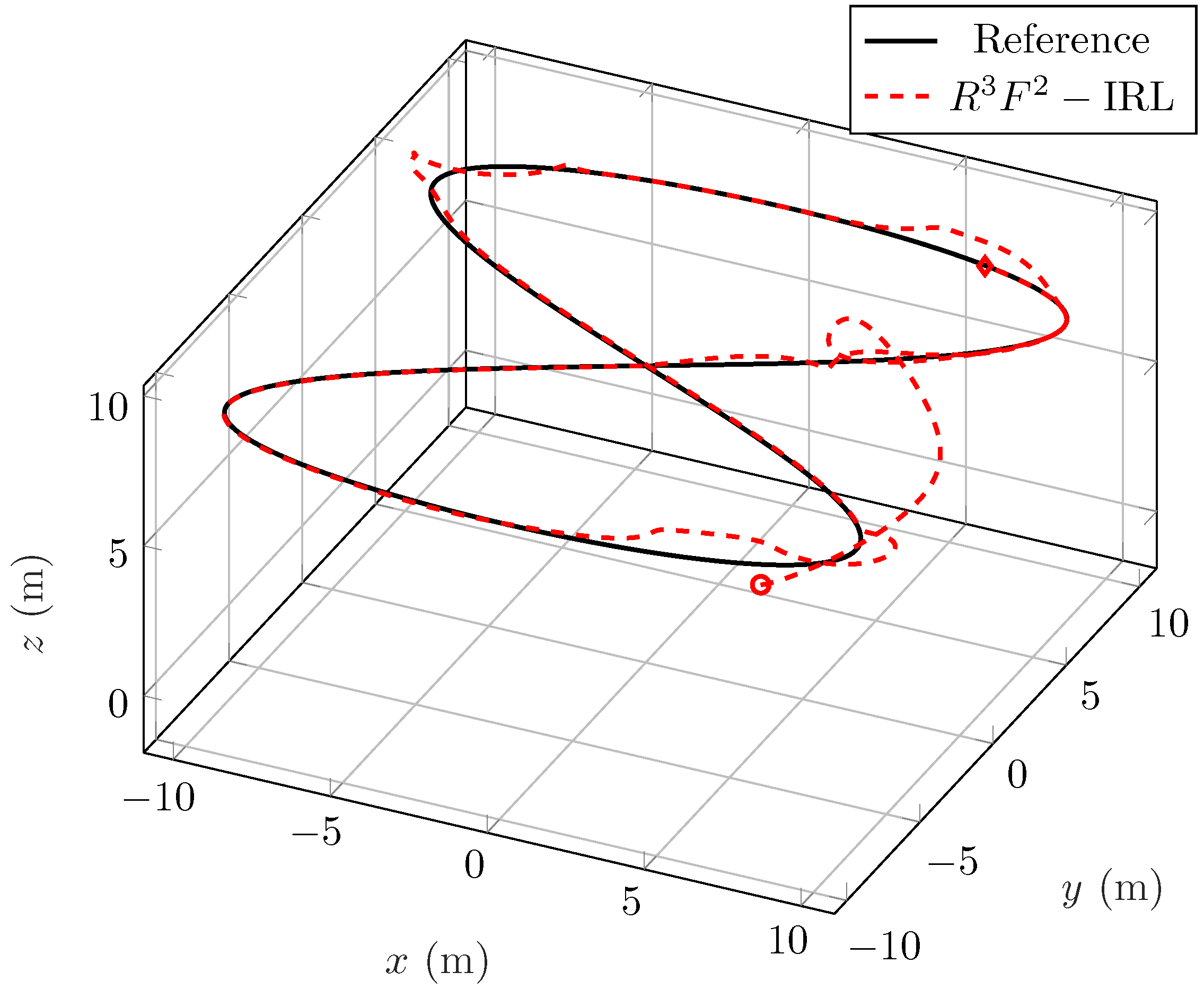
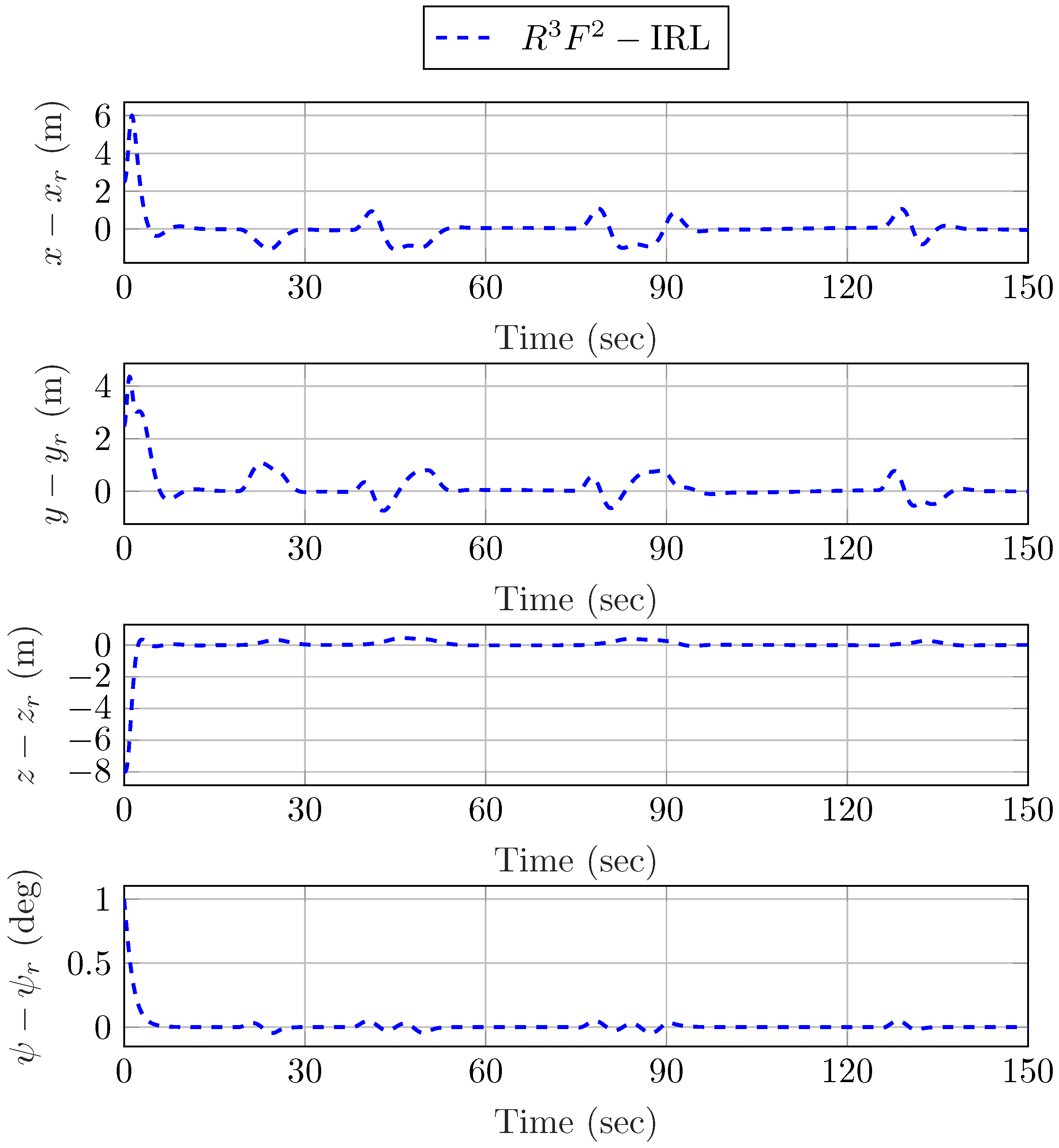
5. Simulation Results

In this section, the performance of the proposed ${\mathrm{R}}^3{\mathrm{F}}^2$-based off-policy IRL scheme will be verified via several simulated examples, where the performance of the gradient descent RL-based controller is also given for the purposes of control performance comparison. To ensure the simulation setting closely follows real-world conditions, we conduct our tracking examples in a virtual experiment platform called the Robot Operating System (ROS) and the Gazebo robotics simulation environment. The virtual UAV tracking scenario is shown in Figure 2, which features a UAV and a bay land.

The physical parameters in UAV dynamics are listed in

Table 1. Parameters of the UAV in the simulation.

Parameters	m	l	g	${\mathit{I}}_{\mathit{x}}$	${\mathit{I}}_{\mathit{y}}$	${\mathit{I}}_{\mathit{z}}$
Values	$2.33$	$0.4$	$9.8$	$0.16$	$0.16$	$0.32$
Units	$\mathrm{kg}$	$\mathrm{m}$	$\mathrm{m}/{\mathrm{s}}^2$	$\mathrm{N}·\mathrm{m}$	$\mathrm{N}·\mathrm{m}$	$\mathrm{N}·\mathrm{m}$

. The aerodynamic damping coefficients $k_i,i=1,\dots ,6$ are set as $k_1=0.01,k_2=0.01,k_3=0.01,k_4=0.015,k_5=0.015$, and $k_6=0.015$. The anti-torque coefficient is chosen as $c=0.05\mathrm{m}$. The external disturbances acting on the position and the attitude subsystems are defined as

$$d_{\zeta }=d_{\vartheta }\triangleq \left\{\begin{array}{c}a(t),t\in \mathrm{\Gamma }\hfill \\ 0,otherwise\hfill \end{array}\right.$$

where

$$a(t)={[0.2sin(0.1t),0.2cos(0.1t),0.1]}^{\top }$$

and

$$\begin{array}{cc}\hfill \mathrm{\Gamma }& =[T_{sim}/8,T_{sim}/6]\cup [T_{sim}/4,T_{sim}/3]\hfill \\ & \cup [T_{sim}/2,3T_{sim}/5]\cup [5T_{sim}/6,7T_{sim}/8]\hfill \end{array}$$

with $T_{sim}=150\mathrm{s}$ being the total simulation time.

The parameters in the value function are set as ${\widehat{Q}}_1={\widehat{Q}}_2=1.2I_6$, ${\widehat{R}}_1={\widehat{R}}_2=1.4I_3$, and ${\eta }_1^2={\eta }_2^2=5$. The reference trajectories of the position and yaw angle are selected as ${\zeta }_r={[10sin({\displaystyle \frac{t}{10}}),10sin({\displaystyle \frac{t}{20}}),8]}^{\top }$ and ${\psi }_r=cos(0.5t)$. The initial states of the UAV are $\zeta (0)={[2.5,2.5,0]}^{\top }$, $\dot{\zeta }(0)={[0,0,0]}^{\top }$, $\vartheta (0)={[1,1,1]}^{\top }$, and $\dot{\vartheta }(0)={[0,0,0]}^{\top }$. The sampling time interval $\Delta t$ is set as $0.01\mathrm{s}$. Furthermore, the activation functions for the critic NNs are chosen as the quadratic polynomials with the structure of 6-21-1. For both the actor and the lumped disturbance NNs, the activation functions are chosen as first-order polynomials with the structure of 6-6-3.

Figure 3 shows the trajectories of the UAV in the $xy$ plane while tracking a white-colored figure-eight trajectory over the overall simulation time. The instantaneous positions of the UAV can be found in the subfigures, illustrating successful tracking performance under external disturbance. In Figure 4, Figure 5 and Figure 6, we demonstrate the simulated results of the proposed approach. Specifically, Figure 4 and Figure 5 show the trajectory tracking performance under the proposed tracking control framework. It can be seen from Figure 5 that the positions and attitudes successfully track the given reference. Moreover, the convergence results of the actor-critic-disturbance NN weights are displayed in Figure 6. It can be seen that the convergence is achieved after the 10th iteration, which verifies the theoretical result established in Theorem 2.

To further show the superiority of the proposed approach, we also compare the performance of this method with that of the gradient descent RL-based controller. Figure 7 depicts the comparison results of the tracking errors of the subsystems under the gradient descent RL-based controllers and the learned robust controllers. One can find that the tracking errors exponentially converge to a small neighborhood of the origin, and the learned robust controllers achieve better performance than the RL-based controllers. In addition, the performance index is taken as the average value of the cost during all the simulation time, i.e., ${\overline{J}}_1={\displaystyle \frac{{\int }_{t=0}^T{q}_i\left({\xi }_i(t),u_i(t),v_i(t)\right)dt}{T_{sim}}}$ and ${\overline{J}}_2={\displaystyle \frac{{\int }_{t=0}^T{q}_i\left({\xi }_i(t),u_i(t),v_i(t)\right)dt}{T_{sim}}}$. Then, the quantitative performance comparison is shown in

Table 2. Comparison of the average costs of the gradient descent RL-based controller and $R^3$${\mathrm{F}}^2$-IRL controller.

Average Cost	Gradient Descent RL	${\mathrm{R}}^3{\mathrm{F}}^2$-IRL
${\overline{J}}_1$	$10.20$	$7.6775$
${\overline{J}}_2$	$0.0576$	$0.0582$

. It can be seen that the performance of our method is significantly better than that of the gradient descent RL method in the position control loop, while the performance is almost the same in the altitude control loop. This difference is likely due to the higher nonlinearity in the position control subsystem. Generally, the attitude subsystem behaves more like a linear system, which explains why our method achieves almost identical performance compared with the gradient descent RL-based one. In summary, our method can successfully handle this nonlinearity (or coupling) with improved control performance.

6. Conclusions

In this paper, a novel robust optimal tracking control framework for a nonlinear UAV with unknown disturbances is proposed. By introducing a virtual control law, the UAV robust optimal tracking control problem is formulated as two independent zero-sum differential games. An ${\mathrm{R}}^3{\mathrm{F}}^2$-based IRL algorithm is presented to obtain the optimal control law and the corresponding worst-case disturbance in a data-driven manner. It is also shown that the learned control law and worst-case disturbance converge to the Nash equilibrium strategies. Finally, numerical simulation results are provided to illustrate the effectiveness of the proposed framework. In future work, this methodology will be extended to multi-agent systems or higher-dimensional dynamics and will address scalability challenges for large-scale differential games.

References

1. Zhou, X.; Wen, X.; Wang, Z.; Gao, Y.; Li, H.; Wang, Q.; Yang, T.; Lu, H.; Cao, Y.; Xu, C.; et al. Swarm of micro flying robots in the wild. Sci. Robot. 2022, 7, eabm5954. [Google Scholar] [CrossRef]
2. Hua, H.; Fang, Y. A novel reinforcement learning-based robust control strategy for a quadrotor. IEEE Trans. Ind. Electron. 2022, 70, 2812–2821. [Google Scholar] [CrossRef]
3. Wang, Y.; Lu, Q.; Ren, B. Wind turbine crack inspection using a quadrotor with image motion blur avoided. IEEE Robot. Autom. Lett. 2023, 8, 1069–1076. [Google Scholar] [CrossRef]
4. Ma, Q.; Jin, P.; Lewis, F.L. Guaranteed cost attitude tracking control for uncertain quadrotor unmanned aerial vehicle under safety constraints. IEEE/CAA J. Autom. Sin. 2024, 11, 1447–1457. [Google Scholar] [CrossRef]
5. Wei, Q.; Yang, Z.; Su, H.; Wang, L. Online Adaptive Dynamic Programming for Optimal Self-Learning Control of VTOL Aircraft Systems With Disturbances. IEEE Trans. Automat. Sci. Eng. 2024, 21, 343–352. [Google Scholar] [CrossRef]
6. Tonan, M.; Bottin, M.; Doria, A.; Rosati, G. Analysis and design of a 3-DOF spatial underactuated differentially flat robot. In Proceedings of the 2025 11th International Conference on Mechatronics and Robotics Engineering (ICMRE), Milan, Italy, 27–29 February 2024; IEEE: New York, NY, USA, 2025; pp. 202–207. [Google Scholar]
7. Wang, L.; Su, J. Robust disturbance rejection control for attitude tracking of an aircraft. IEEE Trans. Control Syst. Technol. 2015, 23, 2361–2368. [Google Scholar] [CrossRef]
8. Zhou, Y.; Chen, M.; Jiang, C. Robust tracking control of uncertain mimo nonlinear systems with application to UAVs. IEEE/CAA J. Autom. Sin. 2015, 2, 25–32. [Google Scholar] [CrossRef]
9. Dydek, Z.T.; Annaswamy, A.M.; Lavretsky, E. Adaptive control of quadrotor UAVs: A design trade study with flight evaluations. IEEE Trans. Control Syst. Technol. 2012, 21, 1400–1406. [Google Scholar] [CrossRef]
10. Sun, S.; Romero, A.; Foehn, P.; Kaufmann, E.; Scaramuzza, D. A comparative study of nonlinear MPC and differential-flatness-based control for quadrotor agile flight. IEEE Trans. Robot. 2022, 38, 3357–3373. [Google Scholar] [CrossRef]
11. Jiao, Q.; Modares, H.; Xu, S.; Lewis, F.L.; Vamvoudakis, K.G. Multi-agent zero-sum differential graphical games for disturbance rejection in distributed control. Automatica 2016, 69, 24–34. [Google Scholar] [CrossRef]
12. Smolyanskiy, N.; Kamenev, A.; Smith, J.; Birchfield, S. Toward low-flying autonomous mav trail navigation using deep neural networks for environmental awareness. In Proceedings of the 2017 IEEE/RSJ International Conference on Intelligent Robots and Systems (IROS), Vancouver, BC, Canada, 24–28 September 2017; IEEE: New York, NY, USA, 2017; pp. 4241–4247. [Google Scholar]
13. Wang, Y.; Sun, J.; He, H.; Sun, C. Deterministic policy gradient with integral compensator for robust quadrotor control. IEEE Trans. Syst. Man, Cybern. Syst. 2019, 50, 3713–3725. [Google Scholar] [CrossRef]
14. Petrlík, M.; Báča, T.; Heřt, D.; Vrba, M.; Krajník, T.; Saska, M. A robust uav system for operations in a constrained environment. IEEE Robot. Autom. Lett. 2020, 5, 2169–2176. [Google Scholar] [CrossRef]
15. Guo, Y.; Sun, Q.; Wang, Y.; Pan, Q. Differential graphical game-based multi-agent tracking control using integral reinforcement learning. IET Control Theory Appl. 2024, 18, 2766–2776. [Google Scholar] [CrossRef]
16. Rubí, B.; Morcego, B.; Pérez, R. A deep reinforcement learning approach for path following on a quadrotor. In Proceedings of the 2020 European Control Conference (ECC), Saint Petersburg, Russia, 12–15 May 2020; IEEE: New York, NY, USA, 2020; pp. 1092–1098. [Google Scholar]
17. Ma, H.-J.; Xu, L.-X.; Yang, G.-H. Multiple environment integral reinforcement learning-based fault-tolerant control for affine nonlinear systems. IEEE Trans. Cybern. 2021, 51, 1913–1928. [Google Scholar] [CrossRef]
18. Greatwood, C.; Richards, A.G. Reinforcement learning and model predictive control for robust embedded quadrotor guidance and control. Auton. Robot. 2019, 43, 1681–1693. [Google Scholar] [CrossRef]
19. Mu, C.; Zhang, Y. Learning-based robust tracking control of quadrotor with time-varying and coupling uncertainties. IEEE Trans. Neural Netw. Learn. Syst. 2019, 31, 259–273. [Google Scholar] [CrossRef]
20. Vrabie, D.; Pastravanu, O.; Abu-Khalaf, M.; Lewis, F.L. Adaptive optimal control for continuous-time linear systems based on policy iteration. Automatica 2009, 45, 477–484. [Google Scholar] [CrossRef]
21. Wang, D.; He, H.; Mu, C.; Liu, D. Intelligent critic control with disturbance attenuation for affine dynamics including an application to a microgrid system. IEEE Trans. Ind. Electron. 2017, 64, 4935–4944. [Google Scholar] [CrossRef]
22. Zhao, B.; Shi, G.; Wang, D. Asymptotically stable critic designs for approximate optimal stabilization of nonlinear systems subject to mismatched external disturbances. Neurocomputing 2020, 396, 201–208. [Google Scholar] [CrossRef]
23. Mohammadi, M.; Arefi, M.M.; Setoodeh, P.; Kaynak, O. Optimal tracking control based on reinforcement learning value iteration algorithm for time-delayed nonlinear systems with external disturbances and input constraints. Inform. Sci. 2021, 554, 84–98. [Google Scholar] [CrossRef]
24. Yang, X.; Gao, Z.; Zhang, J. Event-driven H control with critic learning for nonlinear systems. Neural Netw. 2020, 132, 30–42. [Google Scholar] [CrossRef]
25. Song, R.; Lewis, F.L.; Wei, Q.; Zhang, H. Off-policy actor-critic structure for optimal control of unknown systems with disturbances. IEEE Trans. Cybern. 2015, 46, 1041–1050. [Google Scholar] [CrossRef]
26. Yang, X.; Liu, D.; Luo, B.; Li, C. Data-based robust adaptive control for a class of unknown nonlinear constrained-input systems via integral reinforcement learning. Inform. Sci. 2016, 369, 731–747. [Google Scholar] [CrossRef]
27. Modares, H.; Lewis, F.L.; Jiang, Z. H tracking control of completely unknown continuous-time systems via off-policy reinforcement learning. IEEE Trans. Neural Netw. Learn. Syst. 2015, 26, 2550–2562. [Google Scholar] [CrossRef] [PubMed]
28. Luo, B.; Wu, H.; Huang, T. Off-policy reinforcement learning for H control design. IEEE Trans. Cybern. 2015, 45, 65–76. [Google Scholar] [CrossRef] [PubMed]
29. Cui, X.; Zhang, H.; Luo, Y.; Jiang, H. Adaptive dynamic programming for tracking design of uncertain nonlinear systems with disturbances and input constraints. Int. J. Adapt. Control 2017, 31, 1567–1583. [Google Scholar] [CrossRef]
30. Xiao, G.; Zhang, H.; Zhang, K.; Wen, Y. Value iteration based integral reinforcement learning approach for H controller design of continuous-time nonlinear systems. Neurocomputing 2018, 285, 51–59. [Google Scholar] [CrossRef]
31. Zhao, W.; Liu, H.; Lewis, F.L. Robust formation control for cooperative underactuated quadrotors via reinforcement learning. IEEE Trans. Neural Netw. Learn. Syst. 2021, 32, 4577–4587. [Google Scholar] [CrossRef]
32. Zhao, B.; Xian, B.; Zhang, Y.; Zhang, X. Nonlinear robust adaptive tracking control of a quadrotor UAV via immersion and invariance methodology. IEEE Trans. Ind. Electron. 2015, 62, 2891–2902. [Google Scholar] [CrossRef]
33. Lee, T.; Leok, M.; McClamroch, N.H. Geometric tracking control of a quadrotor UAV on SE (3). In Proceedings of the 49th IEEE Conference on Decision and Control (CDC), Atlanta, GA, USA, 15–17 December 2010; pp. 5420–5425. [Google Scholar] [CrossRef]
34. Cooke, R.D. Unmanned Aerial Vehicles: Design, Development and Deployment; John Wiley & Sons: Hoboken, NJ, USA, 2014. [Google Scholar]
35. Wong, J.Y. Theory of Ground Vehicles; John Wiley & Sons: Hoboken, NJ, USA, 2001. [Google Scholar]
36. Spong, M.W.; Hutchinson, S.; Vidyasagar, M. Robot Modeling and Control; John Wiley & Sons: Hoboken, NJ, USA, 2006. [Google Scholar]
37. Corke, P. Robotics, Vision and Control: Fundamental Algorithms in MATLAB; Springer: Berlin/Heidelberg, Germany, 2017. [Google Scholar]
38. Song, R.; Lewis, F.L. Robust optimal control for a class of nonlinear systems with unknown disturbances based on disturbance observer and policy iteration. Neurocomputing 2020, 390, 185–195. [Google Scholar] [CrossRef]
39. Stone, M.H. The generalized weierstrass approximation theorem. Math. Mag. 1948, 21, 167–184. [Google Scholar] [CrossRef]
40. Gao, W.; Jiang, Z.P. Adaptive dynamic programming and adaptive optimal output regulation of linear systems. IEEE Trans. Autom. Control 2016, 61, 4164–4169. [Google Scholar] [CrossRef]
Figure 1. Diagram of a UAV.
Drones 09 00477 g001
Figure 2. The ROS-/Gazebo-based virtual UAV tracking experimental scenarios.
Drones 09 00477 g002
Figure 3. The virtual experimental results of using the proposed game-based robust tracking control method under an eight-shape reference trajectory; (a) t = 0 s . (b) t = 50 s . (c) t = 100 s . (d) t = 150 s .
Drones 09 00477 g003
Figure 4. The UAV and reference trajectory in 3 dimensions, where the red-colored circle denotes the starting position and the same-colored diamond represents the end position.
Drones 09 00477 g004
Figure 5. The UAV trajectories under the learned robust tracking control controller.
Drones 09 00477 g005
Figure 6. Convergence of the actor-critic-disturbance NN weights.
Drones 09 00477 g006
Figure 7. Evolution of the position and yaw angle tracking error. The red dashed line represents the tracking errors under the gradient descent RL-based controllers, while the blue dashed line represents the tracking errors under the learned robust tracking controllers.
Drones 09 00477 g007