Highlights
First implementation of a drone swarm network for aerial protection in civil aviation zones, critical harbors, and restricted air spaces. The primary objective is to prevent unauthorizedintrusions by biological swarms (e.g., birds) or small unmanned aerial vehicles, thereby mitigating potential catastrophic consequences.
What are the main findings?
- There remains a significant research void in civilian applications of unmanned aerial vehicle (UAV) systems for intruding threat interception and defense.
What is the implication of the main finding?
- This study proposes a novel strategy involving the preemptive spatial deployment of UAV swarms within potential threat trajectories.
Abstract
To address the challenges of dispersing aerial targets such as bird flocks at civilian airports and drones conducting low-altitude surveillance in critical areas, including ports and convention centers, this paper proposes a hybrid Artificial Potential Field-Particle Swarm Optimization (APF–PSO) algorithm. The proposed solution integrates the real-time collision-avoidance capability of the artificial potential field method with the global network-optimization characteristics of the particle swarm algorithm to maximize protective coverage. Simulation results demonstrate that the hybrid algorithm achieves optimal performance in dispersion of aerial targets based on protective coverage under safety constraints, confirming its superior performance. The key innovations lie in implementing a dynamic repulsion field with exponential gain for emergency maneuvers, introducing a vertical avoidance module to resolve deadlock issues, and establishing a novel decoupled cooperative paradigm for scalable aerial protection networks.
1. Introduction
Unmanned Aerial Vehicles (UAVs) have emerged as pivotal tools for executing complex missions owing to their high mobility, rapid deployment flexibility, and favorable cost-effectiveness profiles. As operational complexity escalates, collaborative multi-UAV systems have come to constitute a critical research domain, with research focusing on swarm-intelligence architectures, distributed cooperative control paradigms, and autonomous-formation technologies [1]. Algorithmic advancements in distributed optimization, reinforcement learning, and bio-inspired swarm intelligence (e.g., ant colony and artificial bee colony optimization) have demonstrably augmented mission-allocation efficiency, environmental adaptability, and collective survivability [2].
Within this framework, UAV swarms exhibit significant strategic potential in establishing adaptive defense perimeters against unknown aerial intrusions (e.g., irregular drones or evasive aircraft). Through collaborative sensor fusion and spatially optimized saturation coverage, such systems transcend the performance ceilings of isolated platforms and substantially increase the efficacy of area denial [3]. Persistent challenges include resilience to communication latency in dynamic scenarios, distributed real-time decision-making under uncertainty, and verifiable collision-avoidance mechanisms [4]. These constraints necessitate breakthroughs in computationally efficient yet robust cooperative control frameworks.
Conventional defense models including geometry-based or heuristic rule-based approaches exhibit critical limitations in their effectiveness against emergent threats. These deficiencies stem from static environmental assumptions, discrete decision intervals, and inadequate responsiveness to subsecond-scale maneuvering dynamics [5]. While optimization-based formulations provide theoretical rigor via mathematical programming of cooperative deployments, they confront three fundamental limitations: (1) high-dimensional nonlinearity arising from spatial-coordination dependencies, inducing escalations in computational complexity [6]; (2) real-time feasibility constraints requiring tractable solutions within stringent operational timeframes [7]; (3) dynamic collision constraints mandating concurrent optimization of spatial coverage and intra-swarm safety assurance [8]. In the field of defense against low-altitude drone intrusion, multiple interception strategies have been proposed to optimize regional protection efficacy. Conventional single-drone interception mechanisms (e.g., the pure pursuit guidance algorithm described in [9] and the net interception technique described in [10]) demonstrate precise strike capability against point targets, yet their limited defensive coverage and inefficacy against saturation attacks remain challenges. To enhance interception coverage, collaborative interception paradigms have been progressively developed: Ref. [11] established a red–blue confrontation-simulation model based on multi agent reinforcement learning, achieving multitarget cooperative interception through centralized task allocation, though its assumption of a static environment compromises dynamic adaptability. Ref. [12] improved task-allocation efficiency via a game-theoretic target–defender optimization model, but the computational complexity induced by high-dimensional state spaces impedes real-time performance. Consequently, investigating the formation of drone-swarm-based collaborative defense networks/barriers in dynamic real-time environments may enable efficient interception of single or multiple targets.
Prior to elaborating on the cooperative deployment of multi-UAV swarms for dynamic defense networks, it is imperative to clarify that the underlying challenge is fundamentally a cooperative optimization problem subject to stringent temporal constraints. This study focuses on maximizing the collaborative networking effectiveness of UAV swarms with limited temporal costs (i.e., minimizing deployment time), as specifically manifested by the rapid construction of an effective linear interception barrier (defensive wall, in Figure 1) within predefined interception zones in a real-time three-latitude environment without pretraining. This barrier aims to counter transient threats (e.g., approaching unidentified targets and emergent maneuvers). Crucially, the coverage scope (or effective length/density of the barrier) determines the rate of interception success. Through optimization of deployment strategies to form the optimal barrier in minimal time, the interception probability against emergent threats can be significantly enhanced. Currently, optimization of dynamic barrier formation for UAV swarms under real-time constraints remains largely unexplored, presenting a significant gap. This study aims to identify and address this critical challenge. Mainstream optimization algorithms exhibit fundamental limitations: Genetic Algorithms (GA) suffer from premature convergence and computational intensity, hindering real-time performance [13,14]; Simulated Annealing (SA) shows parameter sensitivity and slow convergence, limiting its responsiveness to sudden maneuvers [15,16]; Traditional PSO (Particle Swarm Optimization) and ABC (artificial bee colony algorithm), while responsive, suffer from local optima entrapment and lack physical constraint modeling [17,18,19,20,21] (e.g., obstacle avoidance).
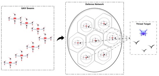
Figure 1.
Schematic diagram of UAV swarm forming a defense network.
Current research demonstrates that hybrid algorithms significantly enhance multi-UAV system performance through heterogeneous optimization paradigms. Reference [22] proposed a centralized–distributed hybrid architecture, integrating the Jonker–Volgenant auction algorithm with iterative optimization to achieve dynamic task allocation for 100 UAVs across 50 targets in firefighting scenarios, improving computational efficiency by 40% while maintaining complexity; however, that work did not address dynamic obstacle avoidance. Reference [23] designed a genetic hill-climbing hybrid algorithm enhanced by population-catastrophe mechanisms, accelerating convergence by 300% and reducing path cost by 14.3% and thus validating synergistic gains in solution quality and stability from heterogeneous integration. Reference [24] developed a hierarchical ABC-A framework* wherein an artificial bee colony generates sparse waypoints refined by A*, increasing the efficiency of threat avoidance by 79% (threat cost reduced from 581.3 to 124.8); however, real-time replanning in 3D environments remains constrained by offline iteration. Reference [25] constructed an HPSO–ant colony hybrid model that adaptively handles capacity-constrained target allocation (payload ≤15), shortening total path length by 27.5% with computation times of 3.08 s, though its assumptions of a static environment are insufficient in the face of emergent obstacles. Collectively, these works confirm that hybrid strategies balance global optimization and real-time response via physical-constraint decoupling (e.g., separating centralized allocation from decentralized execution) and adaptive parameter tuning (e.g., fractional-order PSO). Nevertheless, these fundamental limitations persist in real-time 3D dynamic obstacle-avoidance scenarios: high-dimensional state–space exploration for dynamic obstacle interactions, local optima traps in non-convex obstacle fields, and millisecond-level decision latency in multi agent coordination. Novel hybrid architectures are urgently needed in the quest to achieve deep integration of tactical-level real-time evasion and strategic-level path optimization.
Based on the complementary advantages of different algorithms, multi algorithm-fusion schemes demonstrate enhanced feasibility in experimental implementation. For real-time obstacle avoidance in three-dimensional environments, the classical artificial potential field (APF) [26] method is prioritized. Simultaneously, particle swarm optimization (PSO) [27] is adopted as the primary approach for trajectory-optimization problems. Owing to its predefined velocity and direction parameters for each particle, this algorithm enables rapid deployment in 3D environments. Therefore, we integrate APF with PSO through a dual-layer architecture: the PSO layer handles global optimization of interception paths, while the APF layer provides real-time repulsive fields for collision/obstacle avoidance. This hybrid approach delivers synergistic advantages: potential field gradients guide particles away from local optima; physical constraints reduce high-dimensional search complexity; and the cascade structure balances real-time response with robustness. Specifically, PSO provides strategic global optimization, while APF injects tactical collision rules through velocity–field coupling, dynamically enforcing safety margins during deployment.
The rest of this paper is structured as follows: Section 2 details the methodology, including the threat-kinematics model, the cooperative interception network, the hybrid APF–PSO algorithm design, the construction of an artificial potential field, and the two-phase optimization strategy incorporating a state machine and queue management. Section 3 presents the quantification of defense effectiveness, the calculation of coverage efficiency, and the Voronoi diagram model. Section 4 discusses the hybrid algorithm’s advantages, limitations, and significance, along with future research directions. Section 5 concludes the paper.
2. Methods
2.1. Threat-Target Kinematic Model
In passive defense systems for drone swarms, spatiotemporal prediction of unknown intruders forms the basis for deploying adaptive protective barriers. Low-altitude targets (e.g., bird flocks) typically exhibit aggregated flight behavior. Prior to dispersion operations, real-time tracking of the targets’ three-dimensional (3D) position is required. We achieve this real-time position tracking using ground-based radar. Concurrently, to reduce computational complexity, the targets’ motion model is defined as a uniform linear motion model. This model is described as follows:
The position of the target at time t after its initial detection is denoted by the vector . The constant speed of the target is denoted as , and its direction of motion is determined by the vector from to . Here, represents the target’s position at the time of initial detection, and denotes the position of the protected asset (located at the origin).
However, unlike active interception systems that relocate threat engagements away from the protected target, passive interception systems should position the protective barrier in close proximity to the protected target to minimize potential hazards. Consequently, establishing this barrier necessitates defining an anchor point as a geometric point at a predetermined distance from the protected target . The drone swarm collaboratively navigates to the two-dimensional plane containing , disperses, and assembles into a defensive network.
By definition, lies on the threat target’s flight trajectory. The drones collaboratively assemble into a distributed network at , ensuring high interception success. The parameter determines the position of , and its magnitude directly influences the efficiency of swarm coordination. For computational tractability, in Section 3.1.1, we set to balance simulation runtime, visualization clarity, and buffer-time allocation for potential defense failures. Figure 2 schematically illustrates the threat model with annotated parameters.
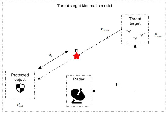
Figure 2.
Threat-target kinematic model.
2.2. Construction of an Artificial Potential Field
2.2.1. Classical Potential Field Model
The Artificial Potential Field (APF) method [26], first proposed by Khatib in 1986, is a classical approach to real-time robot path planning and obstacle avoidance. Its core concept involves modeling the environment through virtual potentials: attractive fields pull agents toward goals, while repulsive fields push them away from obstacles. In UAV swarm coordination, APF is widely adopted for formation keeping and dynamic collision avoidance due to its computational efficiency and clear physical interpretation. The traditional attractive field employs a quadratic function, as follows:
The attractive potential energy is defined such that: denotes the attractive gain coefficient, which governs the strength of the potential field; represents the squared Euclidean distance between the current position of UAV i at and the target point . The attractive force is defined as the negative gradient, as follows:
The attractive force is defined as the negative gradient of the attractive potential energy , with its direction always being toward the target . The repulsive field between UAVs i and j is described by a piecewise function, as follows:
And the repulsive force is defined as follows:
where denotes the maximum effective sensing radius (repulsion activates only when ). As shown in Figure 3, the repulsive force vector exerted on UAV i by UAV j is oriented away from the position of UAV j, and governs the repulsion intensity with superlinear growth as distance decreases.
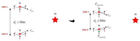
Figure 3.
The goal is unattainable.
Therefore, the total force acting on UAV i is given by the following:
Despite its efficiency in real-time avoidance, this model suffers from three inherent drawbacks:
- Symmetric deadlock: While navigating towards the target, the UAV is subjected to an attractive force from the target and repulsive forces from obstacles or other threats. The UAV reaches an equilibrium state when the net force (vector sum) acting on it equals zero.
- Goal unreachable: When a UAV swarm navigates towards a common target, an individual UAV near the target experiences omnidirectional repulsive forces from surrounding UAVs. Under such conditions, the attractive force exerted on it by the target may be insufficient to counterbalance the resultant repulsive force. This can lead to the phenomenon of target inaccessibility.
- Path oscillation: Dynamic imbalance between attraction or repulsion causes trajectory jitter.
2.2.2. Optimized Design Scheme for a Potential Field
When multiple UAVs are approaching the target, they may become dominated by repulsive forces, resulting in target inaccessibility and oscillatory phenomena during flight, as shown in Figure 4.
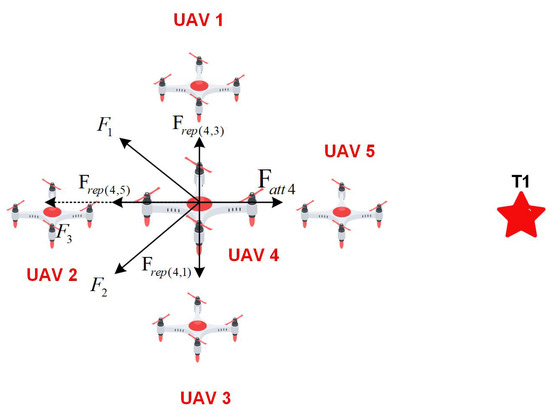
Figure 4.
Target inaccessibility.
As illustrated in Figure 4, UAV 4 experiences repulsive forces from UAV 1, UAV 2, UAV 3, and UAV 5, while simultaneously being subjected to an attractive force from target . In the figure, denotes the resultant repulsive-force vector exerted on UAV 4 by UAV 1 and UAV 2; denotes the resultant repulsive-force vector exerted on UAV 4 by UAV 3 and UAV 5; represents the total resultant repulsive-force vector acting on UAV 4 (i.e., the vector sum of repulsive forces from all surrounding UAVs); denotes the attractive-force vector exerted on UAV 4 by target . In this depicted scenario, the magnitude of may exceed the magnitude of , and, crucially, the direction of the net force may point away from the target. This condition can prevent the UAV from reaching target .
BinKai et al. [28] introduced a dynamic regulation factor into the conventional attractive-potential function to balance abrupt changes between attraction and repulsion, thereby mitigating the goal-unreachable problem. Zhang et al. [29] redesigned the repulsive function such that repulsion attenuates when agents approach targets and transitions smoothly when agents are gaining distance from obstacles, effectively suppressing motion chattering. Both strategies aim to eliminate oscillatory behaviors in potential fields. Inspired by these advances, we reconstruct the repulsive and attractive field functions to expedite deployment: enhanced intensity of near-field repulsion prevents UAV-aggregation-induced slow convergence.
Thus, within the effective range, the repulsive potential field function is formulated as:
In the potential field function, the core repulsive term exhibits the following properties:
- Both the logarithmic term and the inverse term monotonically increase as decreases, synergistically amplifying repulsion;
- The offset term ensures the core term vanishes at , guaranteeing smooth transitions at potential field boundaries.
Furthermore, the dynamic gain factor gives the following:
- Significant repulsion amplification (up to 6×) at close range (), enhancing the robustness of obstacle avoidance;
- Asymptotically attenuated gain (approaching unity) when , preventing unnecessary repulsive interference.
This design achieves substantial improvements in collision avoidance while effectively suppressing motion oscillations induced by abrupt force transitions.
Figure 5 illustrates the force-analysis diagram of UAV swarms, where the resultant force acting on each UAV is depicted with directional arrows, explicitly visualizing the dynamic coupling between attractive and repulsive potentials.
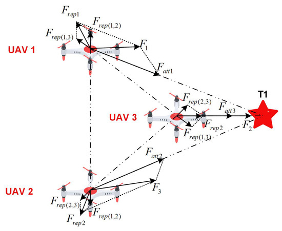
Figure 5.
Force-analysis diagram.
To address the local-minimum problem (i.e., deadlock phenomenon), Xie et al. [30] modeled the environment via potential fields, where reward functions (e.g., increasing rewards when approaching targets) drive optimal action learning to escape local traps; Liu et al. [31] combined improved A* with potential fields, using A* for global path generation and potential fields for local obstacle avoidance. However, these approaches either incur high computational costs or rely on extensive training samples, compromising real-time performance and robustness. Therefore, prioritizing real-time operation and scalability, we propose a random vertical-escape-force mechanism, as shown in Figure 6, to efficiently overcome local minima.
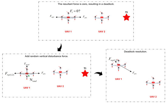
Figure 6.
Symmetrical position adds obstacle-avoidance force.
And the random vertical escape force is designed as follows:
where defines the direction of the deadlock axis. By computing the cross-product of the relative position vector and a random unit vector , an escape-force vector is generated that is simultaneously orthogonal to both the deadlock axis and . indicates that the random variable follows a continuous uniform distribution over the interval . It should be emphasized that this escape force exhibits non-deterministic characteristics: the randomly generated escape direction may induce the formation of additional instabilities. Nevertheless, the repulsive potential field incorporates an exponential repulsive gain at close range, where repulsion intensifies drastically as interdrone distance decreases, thereby fundamentally preventing aggregation behavior.
Furthermore, we redesigned the attractive potential field to incorporate velocity constraints, ensuring smooth UAV trajectories while preventing aggregation induced by excessive speed, thereby effectively suppressing oscillatory behavior.
In this scheme, implementing linear growth of the potential energy effectively prevents the attractive force from increasing indefinitely with distance. This avoids situations where UAVs accelerate excessively toward the target in far-field regions due to an overly large potential gradient, thereby eliminating the risk of collision during path convergence.
2.3. Hybrid Algorithm Design
Particle Swarm Optimization (PSO) [27] achieves global optimization through swarm intelligence, with position and velocity update rules defined as follows:
where is the optimal position discovered by the entire swarm, driving convergence toward the global optimum; represents the historical optimum of individual particles, preserving the capacity for local exploration; and w balances historical velocity and current guidance (); regulate the influence of individual and collective experience (typically ); and are uniformly distributed random numbers in , enhancing exploratory randomness.
In the PSO algorithm, while the velocity-update formula is clearly defined, its stochastic search mechanism requires special consideration when it is applied to actual drone flights: motion trajectories must maintain smoothness, and interparticle collisions must be strictly prevented. Notably, the improved APF method comprehensively addresses both obstacle avoidance and path guidance. The global convergence of the reconstructed hybrid algorithm is thoroughly discussed in Section 2.5.
Therefore, we integrate PSO’s inertia mechanism with APF’s gradient theory, as follows:
where , corresponds to in PSO, acting as the global attractor that guides the UAV toward the target position, and corresponds to in PSO, functioning as the local optimizer for real-time obstacle avoidance. This position/velocity update preserves the canonical PSO formulation, thereby guaranteeing theoretical convergence of the optimization process.
2.4. Two-Phase Optimization
Building upon the improved potential field- -PSO hybrid algorithm (guaranteeing balanced flight, collision avoidance, and oscillation suppression), the interception model centers on the critical node : once any UAV reaches , others immediately form a cooperative 2D defensive screen centered at this point. This two-phase mechanism comprises the following:
- Assembly Phase: Guiding the swarm to converge at target . During this phase, the attraction target in the potential field for every UAV is set to this shared point (i.e., ).
- Readiness–Deployment Phase: Upon first UAV arrival at , the remaining UAVs enter a dynamic allocation mode. Each UAV is sequentially assigned a unique, static deployment point on the defensive plane, calculated relative to . Subsequently, the attraction target for each of these UAVs is updated from the shared to an individual (i.e., ), guiding them to form an optimal defensive network.
For any UAV i, its velocity update follows:
where is the velocity inertia coefficient, is the potential field gradient gain coefficient, and represents the composite potential field gradient at position . Planar arrival is triggered when any UAV i satisfies the following:
Here, is the unit normal vector of the interception plane, determined by the direction of the threat trajectory. This event triggers UAV to its final hovering state while activating the ready–deployment phase for others. The deployment priority queue is defined as follows:
and:
The head UAV acquires its target position through polar coordinate sampling:
where are orthogonal basis vectors generated by cross products of the threat direction vector. Candidate points are discretized on a grid:
With safety filtering:
Then, the optimal deployment point is selected as follows:
Let r and denote the radial distance and azimuth angle in the polar coordinate system centered at . The discrete grid is generated with indices k (radial steps) and l (angular steps), where , . The safety radius defines the minimum clearance to any obstacle position . And is the final deployment target point of the current UAV.
2.5. Convergence Analysis
The classic PSO convergence condition requires [32]. In the hybrid algorithm, we removed the random terms and replaced them with deterministic potential field gradients, so this convergence condition is no longer directly applicable. However, it is worth noting that if we treat the potential field gradient term as the social term in PSO (i.e., setting , ), the convergence condition transforms into . Our chosen parameters , satisfy . This can serve as a reference. This paper employs the following hybrid dynamics equation during the deployment phase:
where the total potential field exhibits dual mathematical properties: is -strongly convex at target positions , ensuring optimization directionality, and is L-Lipschitz smooth, preventing gradient explosion. From convex optimization theory, the algorithm converges to stable points at a rate of , a conclusion rigorously proven via the Banach fixed-point theorem [33].
Furthermore, as shown in Table 1, extensive experimental results demonstrate convergent behavior of the hybrid algorithm, providing additional empirical validation for its convergence properties.

Table 1.
Comparison of algorithms for multi-UAV coverage optimization.
2.6. Voronoi Diagram Model
A Voronoi diagram partitions a plane into convex polygons (cells) based on a set of generators, where each cell contains all locations closer to its generator than to any other [34]. This property is particularly suitable for straightforward target-assignment tasks, especially in constructing passive defense networks. In this study, when a threat target is located within a specific Voronoi cell, the corresponding drone can be directly assigned for interception. This approach eliminates the need for conflict resolution and avoids complex real-time task-allocation strategies, providing a simple yet reliable solution, as shown in Figure 7a.
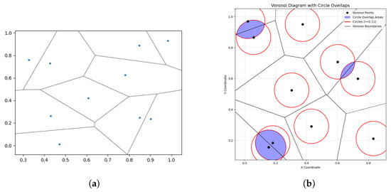
Figure 7.
(a) Each point represents a drone’s position, with the surrounding polygon defining its Voronoi cell. (b) In drone swarms, coverage areas may extend beyond Voronoi boundaries, creating overlapping regions.
However, this optimal coverage scheme has limitations: with fixed coverage per drone, Voronoi construction may cause resource waste due to overlapping regions, as shown in Figure 7b.
For coverage-optimization problems, regular hexagonal grids represent the theoretical optimal solution for maximizing area coverage in Figure 8a, as rigorously established by the Honeycomb Conjecture proved by Hales (1999) [35]. Within our drone defense framework, this hexagonal Voronoi configuration defines the theoretical maximum defensive coverage area, serving as a benchmark for swarm-deployment efficiency.
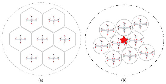
Figure 8.
(a) The theoretically optimal Voronoi configuration consists of regular hexagonal cells. (b) During actual deployment of the defense network, each newly added drone is positioned closer to the target than the next deployed drones.
Critically, this coverage model serves only as a reference in experiments. During actual interception, coverage expansion—to accommodate unforeseen scenarios like sudden trajectory changes—must be secondary to ensuring effective target neutralization. This requires maintaining sufficient density in the interception zone. Thus, while optimal coverage points can theoretically be predetermined based on drone count to guide positioning, individual drone decisions alone cannot guarantee interception effectiveness.
Figure 8b demonstrates the optimized defense network: each drone’s position ensures proximity superiority to subsequent drones relative to the target, maximizing interception efficacy.
3. Results
3.1. Simulation Validation
3.1.1. Experimental Setup and Main Process
To ensure statistical robustness and reproducibility while avoiding coincidental results, the UAV initialization parameters are configured as follows:
- Initialization area: A cubic region defined by minimum bounds [] (m) and maximum bounds [50, 50, 50] (m) in the x–y–z coordinate system, with randomized takeoff positions generated uniformly within this volume.
- Target parameters: (1) speed: m/s; (2) initial position: (m); (3) terminal position: (m).
- Detection parameters: (1) initial intercept distance: m from origin; (2) intercept plane normal vector: computed from target trajectory vector; (3) maximum detection range of UAV: . (4) defensive coverage radius: m.
- Other details: . (These values are for reference only, and no sensitivity analysis has been conducted.)
From the trajectory visualization, we observe that during the initial phase, all UAVs consistently navigate toward the common target . Upon the first UAV reaching the interception plane, subsequent optimization activates, prompting the UAVs to strategically disperse around the collision point. This dispersion forms an optimized planar defense network, significantly expanding the protected area while ensuring interception effectiveness. The pink shaded regions represent the effective coverage radius of individual UAVs, illustrating their spheres of influence within the collective defense system. When the system scales to 15 UAVs, as shown in Figure 9a,b, we conduct detailed analysis of swarm dynamics, as follows:
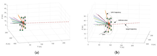
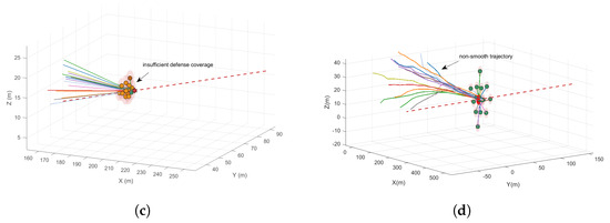
Figure 9.
(a) Spatially distributed interception network formed by 15 autonomous UAVs via the hybrid APF−PSO algorithm. (b) Side view of the defense network, including the flight route of the unmanned aerial vehicle. (c) Spatially distributed interception network formed by 15 autonomous UAVs via the hybrid APF algorithm. (d) Spatially distributed interception network formed by 15 autonomous UAVs via the hybrid IPSO (Improved PSO) algorithm.
During the optimization of the deployment phase on the interception plane, UAVs consistently prioritize collision avoidance with swarm members while simultaneously seeking optimal positions that minimize distance to the critical interception point , resulting in an emergent formation that converges to a quasi-circular planar arrangement. This geometric configuration maximizes defense coverage area while maintaining optimal interception probability, achieving peak cost-effectiveness through balanced spatial coverage and resource-utilization efficiency. Furthermore, the formation stability demonstrated throughout this process confirms the algorithm’s robust capability to handle increased swarm density without performance degradation, even under high-density spatial-optimization conditions.
For comparison, we also present the performance results from using the APF, as shown in Figure 9c approach and the improved PSO scheme shown in Figure 9d. In the APF solution, we observe that the UAV swarm maneuvers toward the interception point, eventually oscillating near the designated interception plane due to competing attraction and repulsion forces from multiple directions, which leads to a sharp increase in time complexity. In the visualization, UAVs are shown in green when they are entering hover state, while the amber color indicates they are still optimizing toward the target. Overall, when the target reaches interception point , the resulting defense network exhibits clustered formations, indicating poor defensive effectiveness.
As for the standard PSO approach, since it does not inherently consider collision avoidance during iterations and is prone to local optima, we implemented an improvement: during each iteration, the UAV with the highest fitness value is identified as the optimal agent and receives an additional attraction force toward the interception point. This modification helps guide the swarm toward the global optimum. We term this modified algorithm the improved particle swarm optimization (IPSO) algorithm, as shown in Figure 9d. The results demonstrate that compared to our hybrid approach, the IPSO solution generates less smooth UAV trajectories, reflecting its inferior temporal performance due to iterative influences.
In summary, preliminary evaluation based on visual comparisons across different algorithmic approaches suggests that the hybrid algorithm demonstrates superior performance metrics.
3.1.2. Quantitative Performance Metrics
To ensure experimental rigor, we conducted the following tests: for each scenario with 5, 10, 15, 20, and 25 UAVs respectively, we performed 50 independent experimental trials in Table 1 and Figure 10. We quantitatively evaluated the following key performance metrics. (1) Average defense area. (2) Average computation time (the computation time refers to the actual CPU time consumed by the algorithm from initialization to completion of the entire simulation process, which depends on CPU performance and reflects the computational efficiency of the algorithm. This metric enables horizontal performance comparison between different algorithms but does not represent the actual physical operation time in the real world. In this experiment, each iteration of the algorithm is defined to last 0.1s (dt = 0.1 s). All timing measurements were conducted using an AMD R7-4700U processor (Advanced Micro Devices, Inc., Santa Clara, CA, USA; 2.00 GHz base clock) with MATLAB R2022a’s tic-toc timing framework to ensure consistency across trials). (3) Average number of safety violations. (4) Average number of collisions.
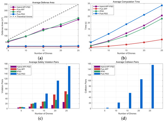
Figure 10.
(a) The line plot depicting the relationship between average defense coverage area and UAV swarm size. (b) The trend in computational duration versus the number of unmanned aerial vehicles. (c) Pattern of variation in the logarithmic value of the number of security-breach incidents with increasing UAV quantity. (d) Correlation curve between collision frequency and size of the drone population.
This experimental setup models UAVs as point-mass entities and does not account for practical physical constraints, aiming specifically to assess the feasibility of the core algorithm in its preliminary stage.
In the 15-UAV application scenario, the Hybrid APF–PSO algorithm demonstrates balanced optimization across multidimensional performance metrics. According to Table 1, compared to IPSO (9.66 s), Hybrid APF–PSO (11.71 s) increased computation time by 21.2% but achieved a larger defense area (150.78 m2 vs. 142.61 m2), with an improvement of 8.17 m2 (5.73%), demonstrating sustained superiority in coverage efficiency and reflecting a trade-off between computational cost and performance enhancement. This confirms the algorithm’s efficacy in circumventing exponential escalation in computational complexity.
Regarding coverage performance, the algorithm achieves a detection area of 150.78 m2, outperforming IPSO (142.61 m2) by 5.7%. This corresponds to 11.9× and 8.6× the coverage of Pure APF (12.62 m2) and Pure PSO (17.49 m2), respectively. Per-UAV efficiency reaches 10.05 m2/UAV, exceeding that of IPSO (9.51 m2/UAV) by 5.7%. The final coverage ratio of 72.5% approaches the theoretical maximum (72.5% of the 207.85 m2 Voronoi partition area), demonstrating near-optimal convergence within feasible solution spaces.
Safety performance exhibits more substantial improvements. With only nine airspace violations, reductions of 67.4%, 85.0%, and 68.5% were achieved relative to Pure APF (27.6), Pure PSO (60.1), and IPSO (28.6), respectively. Notably, zero collisions occurred (versus 55.5 collisions for Pure PSO), highlighting robust obstacle avoidance in dense swarms.
Comprehensive evaluation reveals the algorithm’s area–time ratio (12.9 m2/s) ranks second to that of IPSO (14.8 m2/s) but substantially exceeds those of Pure APF (4.3 m2/s) and Pure PSO (0.93 m2/s). Its area-per-violation ratio (16.8 m2/violation) dramatically surpasses those of benchmark algorithms (Pure APF: 0.46; Pure PSO: 0.29; IPSO: 5.0). These results establish a Pareto-optimal balance among coverage efficiency, safety constraints, and computational resource consumption in medium-scale swarms, validating its non-trivial performance trade-off characteristics.
4. Discussion
This study proposes a hybrid APF–PSO algorithm for UAV swarm defense against high-speed aerial threats. The key innovations include the following: (1) a dual-layer control architecture decoupling global path optimization (PSO) from real-time collision avoidance (APF); (2) dynamic repulsive fields with exponential gain coefficients enabling 10 ms emergency response; (3) vertical perturbation forces resolving symmetrical deadlocks; and (4) a two-phase state machine with ready queue management.
Experimental validation confirms that the 15-drone Hybrid APF–PSO configuration optimally balances coverage efficiency (150.78 m2, 72.5% of theoretical maximum), computation time (11.71 s), and safety metrics (9.00 violations/run with zero collisions). This demonstrates a 6.7–9.2% coverage improvement over suboptimal configurations (20 and 25 drones) while maintaining collision-free operations, achieving a cost-effectiveness ratio of 10.05 m2/UAV; in this respect, the configuration outperforms existing methods in real-time deployability.
Future research will focus on the following points: (1) adaptive learning extensions for dynamic threat environments, such as reinforcement learning and deep reinforcement learning; (2) distributed consensus protocols for >25-drone swarms; and (3) multilayer 3D deployment to enhance coverage efficiency beyond planar limitations, approaching theoretical limits. The proposed method establishes a foundation for scalable aerial defense networks with verifiable safety guarantees.
5. Conclusions
Our work establishes a fundamentally new paradigm for aerial threat defense by introducing the first hybrid framework that unifies strategic coverage maximization with real-time collision-free deployment. This approach differs radically from prior solutions in three aspects:
- Architectural novelty: Existing methods prioritize either global optimization or reactive avoidance, but fail to integrate both. Our APF–PSO hybrid is the first to embed PSO’s global waypoints into continuous potential fields via mechanical decomposition , enabling simultaneous path optimization and physics-compliant navigation.
- Queue-managed state-transition mechanism: This ensures conflict-free sequential execution among multiple UAVs, thereby simplifying task assignment.
- Zero collisions: This was maintained across all trials (N = 5–25), even while minimum spacing was maintained at >0.1 m (Figure 10), resolving the “safety-coverage tradeoff” that plagues rule-based systems.
- Cost-effective scalability: The 15-drone configuration delivers 150.78 m2 coverage at 10.052 m2/UAV—a 10.3% improvement over 25-drone deployments (Table 1), proving feasibility for resource-constrained operations.
Author Contributions
Funding acquisition, Conceptualization, L.Z.; Software, Validation and Writing—original draft, Y.W.; Formal analysis, Project administration, and Writing—review and editing, Y.L. and R.G.; Methodology, L.Z. and R.G. All authors have read and agreed to the published version of the manuscript.
Funding
This research is funded by the National Natural Science Foundation of China (Grant No. 62473373).
Data Availability Statement
Data are contained within the article.
Conflicts of Interest
The authors declare no conflicts of interest.
References
- Liang, J.; Miao, H.; Li, K.; Tan, J.; Wang, X.; Luo, R.; Jiang, Y. A Review of Multi-Agent Reinforcement Learning Algorithms. Electronics 2025, 14, 820. [Google Scholar] [CrossRef]
- Tang, J.; Liu, G.; Pan, Q. A Review on Representative Swarm Intelligence Algorithms for Solving Optimization Problems: Applications and Trends. IEEE/CAA J. Autom. Sin. 2021, 8, 1627–1643. [Google Scholar] [CrossRef]
- Liu, X.; Guo, J. Review of UAV Based on Reconfigurable Intelligent Surface and ISAC. Sci. J. Intell. Syst. Res. 2025, 7, 1–11. [Google Scholar] [CrossRef]
- Faria, R.; Capron, B.; De Souza, M., Jr.; Secchi, A. One-Layer Real-Time Optimization Using Reinforcement Learning: A Review with Guidelines. Processes 2023, 11, 123. [Google Scholar] [CrossRef]
- Wang, R.; Tang, S. Intercepting Higher-Speed Targets Using Generalized Relative Biased Proportional Navigation. J. Northwest. Polytech. Univ. 2019, 37, 682–690. [Google Scholar] [CrossRef]
- Esmin, A.A.A.; Coelho, R.A.; Matwin, S. A Review on Particle Swarm Optimization Algorithm and Its Variants to Clustering High-Dimensional Data. Artif. Intell. Rev. 2015, 44, 23–45. [Google Scholar] [CrossRef]
- Lukáš, D.; Kot, T. Hierarchical Real-Time Optimal Planning of Collision-Free Trajectories of Collaborative Robots. J. Intell. Robot. Syst. 2023, 107, 57. [Google Scholar] [CrossRef]
- Ryou, G.; Tal, E.; Karaman, S. Cooperative Multi-Agent Trajectory Generation with Modular Bayesian Optimization. arXiv 2022, arXiv:2206.00726. [Google Scholar] [CrossRef]
- Wang, X.; Tan, G.; Dai, Y.; Lu, F.; Zhao, J. An Optimal Guidance Strategy for Moving-Target Interception by a Multirotor Unmanned Aerial Vehicle Swarm. IEEE Access 2020, 8, 121650–121664. [Google Scholar] [CrossRef]
- Xiang, H.; Liang, C.; Qiao, Z.; Yuan, X.; Cao, G. Parameters Simulation and Optimization of Flying Net for UAVs Interception. IEEE Access 2022, 10, 56668–56676. [Google Scholar] [CrossRef]
- Song, X.; Yang, R.; Yin, C.; Tang, B. A Cooperative Aerial Interception Model Based on Multi-Agent System for UAVs. In Proceedings of the 2021 IEEE 5th Advanced Information Technology, Electronic and Automation Control Conference (IAEAC), Chongqing, China, 12–14 March 2021; pp. 873–882. [Google Scholar]
- Tong, B.; Duan, H. A Game Theory-Based Approach for Multiple UAVs Cooperative Target Defense. IEEE Trans. Circuits Syst. II Express Br. 2024, 71, 2149–2153. [Google Scholar] [CrossRef]
- Jeong, I.; Lee, J. Adaptive Simulated Annealing Genetic Algorithm for System Identification. Eng. Appl. Artif. Intell. 1996, 9, 523–532. [Google Scholar] [CrossRef]
- Katoch, S.; Chauhan, S.S.; Kumar, V. A Review on Genetic Algorithm: Past, Present, and Future. Multimed. Tools Appl. 2021, 80, 8091–8126. [Google Scholar] [CrossRef] [PubMed]
- Jie, S.; Hu, Z.; Chun-Lin, S. Simulated Annealing Algorithm Based on Gauss Distribution. Sci. Discov. 2016, 4, 52. [Google Scholar] [CrossRef][Green Version]
- Suman, B.; Kumar, P. A Survey of Simulated Annealing as a Tool for Single and Multiobjective Optimization. J. Oper. Res. Soc. 2006, 57, 1143–1160. [Google Scholar] [CrossRef]
- Bai, Y.; Ruan, Z. Application of Automatic Driving Task Sequentialisation Monitoring for Band Operator Robots. Appl. Math. Nonlinear Sci. 2024, 9, 20241437. [Google Scholar] [CrossRef]
- Girija, S.; Joshi, A. Fast Hybrid PSO-APF Algorithm for Path Planning in Obstacle Rich Environment. IFAC-PapersOnLine 2019, 52, 25–30. [Google Scholar] [CrossRef]
- Shankar, M.; Sushnigdha, G. A Hybrid Path Planning Approach Combining Artificial Potential Field and Particle Swarm Optimization for Mobile Robot. IFAC-PapersOnLine 2022, 55, 242–247. [Google Scholar] [CrossRef]
- Alqudsi, Y.; Makaraci, M. Towards Optimal Guidance of Autonomous Swarm Drones in Dynamic Constrained Environments. Expert Syst. 2025, 42, e70067. [Google Scholar] [CrossRef]
- Huang, S.; Zhang, H.; Huang, Z. E2CoPre: Energy Efficient and Cooperative Collision Avoidance for UAV Swarms with Trajectory Prediction. arXiv 2023, arXiv:2303.06510. [Google Scholar]
- Luna, M.A.; Refaat Ragab, A.; Ale Isac, M.S.; Flores Peña, P.; Cervera, P.C. A New Algorithm Using Hybrid UAV Swarm Control System for Firefighting Dynamical Task Allocation. In Proceedings of the 2021 IEEE International Conference on Systems, Man, and Cybernetics (SMC), Melbourne, Australia, 17–20 October 2021; pp. 655–660. [Google Scholar]
- Tian, J.; Wang, Y.; Fan, C. Research on Target Assignment of Multiple-UAVs Based on Improved Hybrid Genetic Algorithm. In Proceedings of the 2018 IEEE 4th International Conference on Control Science and Systems Engineering (ICCSSE), Wuhan, China, 21–23 August 2018; pp. 304–307. [Google Scholar]
- Bai, X.; Wang, P.; Wang, Z.; Zhang, L. 3D Multi-UAV Collaboration Based on the Hybrid Algorithm of Artificial Bee Colony and A*. In Proceedings of the 2019 Chinese Control Conference (CCC), Guangzhou, China, 27–30 July 2019; pp. 3982–3987. [Google Scholar]
- Bi, J.; Huang, W.; Li, B.; Cui, L. Research on the Application of Hybrid Particle Swarm Algorithm in Multi-UAV Mission Planning with Capacity Constraints. In Proceedings of the 2024 IEEE International Conference on Unmanned Systems (ICUS), Nanjing, China, 18–20 October 2024; pp. 928–933. [Google Scholar]
- Khatib, O. Real-Time Obstacle Avoidance for Manipulators and Mobile Robots. In Proceedings of the 1985 IEEE International Conference on Robotics and Automation, St. Louis, MO, USA, 25–28 March 1985; Institute of Electrical and Electronics Engineers: St. Louis, MO, USA, 1985; Volume 2, pp. 500–505. [Google Scholar]
- Kennedy, J.; Eberhart, R. Particle Swarm Optimization. In Proceedings of the ICNN’95—International Conference on Neural Networks, Perth, WA, Australia, 27 November–1 December 1995; Volume 4, pp. 1942–1948. [Google Scholar]
- BinKai, Q.; Mingqiu, L.; Yang, Y.; Xiyang, W. Research on UAV Path Planning Obstacle Avoidance Algorithm Based on Improved Artificial Potential Field Method. J. Phys. Conf. Ser. 2021, 1948, 012060. [Google Scholar] [CrossRef]
- Zhang, P.; Wang, Z.; Zhu, Z.; Liang, Q.; Luo, J. Enhanced Multi-UAV Formation Control and Obstacle Avoidance Using IAAPF-SMC. Drones 2024, 8, 514. [Google Scholar] [CrossRef]
- Xie, L.; Xie, G.; Chen, H.; Li, X. Solution to Reinforcement Learning Problems with Artificial Potential Field. J. Cent. South Univ. Technol. 2008, 15, 552–557. [Google Scholar] [CrossRef]
- Liu, L.; Wang, B.; Xu, H. Research on Path-Planning Algorithm Integrating Optimization A-Star Algorithm and Artificial Potential Field Method. Electronics 2022, 11, 3660. [Google Scholar] [CrossRef]
- Qian, W.; Li, M. Convergence Analysis of Standard Particle Swarm Optimization Algorithm and Its Improvement. Soft Comput. 2018, 22, 4047–4070. [Google Scholar] [CrossRef]
- Beck, A.; Teboulle, M. A Fast Iterative Shrinkage-Thresholding Algorithm for Linear Inverse Problems. SIAM J. Imaging Sci. 2009, 2, 183–202. [Google Scholar] [CrossRef]
- Okabe, A.; Suzuki, A. Locational Optimization Problems Solved through Voronoi Diagrams. Eur. J. Oper. Res. 1997, 98, 445–456. [Google Scholar] [CrossRef]
- Hales, T.C. The Honeycomb Conjecture. Discrete Comput. Geom. 2001, 25, 1–22. [Google Scholar] [CrossRef]


Disclaimer/Publisher’s Note: The statements, opinions and data contained in all publications are solely those of the individual author(s) and contributor(s) and not of MDPI and/or the editor(s). MDPI and/or the editor(s) disclaim responsibility for any injury to people or property resulting from any ideas, methods, instructions or products referred to in the content. |
© 2025 by the authors. Licensee MDPI, Basel, Switzerland. This article is an open access article distributed under the terms and conditions of the Creative Commons Attribution (CC BY) license (https://creativecommons.org/licenses/by/4.0/).