Abstract
Unmanned Aerial Vehicles (UAVs) are increasingly deployed in environmental monitoring, logistics, and precision agriculture. Efficient and reliable path planning is particularly critical for UAV systems operating in 3D continuous environments with multiple obstacles. However, single-UAV systems are often inadequate for such environments due to limited payload capacity, restricted mission coverage, and the inability to execute multiple tasks simultaneously. To overcome these limitations, multi-UAV collaborative systems have emerged as a promising solution, yet coordinating multiple UAVs in high-dimensional 3D continuous spaces with complex obstacles remains a significant challenge for path planning. To address these challenges, this paper proposes a reinforcement-learning-driven multi-strategy continuous ant colony optimization algorithm, QMSR-ACOR, which incorporates a Q-learning-based mechanism to dynamically select from eight strategy combinations, generated by pairing four constructor selection strategies with two walk strategies. Additionally, an elite waypoint repair mechanism is introduced to improve path feasibility and search efficiency. Experimental results demonstrate that QMSR-ACOR outperforms seven baseline algorithms, reducing average path cost by 10–60% and maintaining a success rate of at least 33% even in the most complex environments, whereas most baseline algorithms fail completely with a success rate of 0%. These results highlight the algorithm’s robustness, adaptability, and efficiency, making it a promising solution for complex multi-UAV path planning tasks in obstacle-rich 3D environments.
1. Introduction
In recent years, Unmanned Aerial Vehicles (UAVs) have been widely used in environmental monitoring, logistics, and precision agriculture [1,2,3]. Despite their success, single-UAV systems are inherently limited by payload capacity, restricted mission coverage, and the inability to execute multiple tasks simultaneously, which restricts mission efficiency and scalability. Consequently, multi-UAV collaboration has emerged as a promising solution [4], offering higher efficiency, greater coverage, and improved task flexibility, and has been quickly applied in power line inspection [5], crop protection [6], and disaster relief operations [7].
In multi-UAV systems, efficient path planning is essential to ensure safe, coordinated, and high-performance operations. However, path planning in three-dimensional continuous environments is particularly challenging due to the presence of obstacles and the need for inter-UAV coordination. Researchers have explored various methods for UAV path planning, including cell decomposition, roadmap approaches, potential fields, and evolutionary computation (EC) algorithms [8].
Specifically, cell methods are easy to implement but become inefficient as the resolution of the grid increases. Roadmap methods, such as visibility graphs and probabilistic roadmaps, can create dense graphs in cluttered environments, consuming more memory and computational time. Potential field methods are fast, but easily fall into a local optima, making them unreliable in complex scenarios. More details are provided in Section 2.
As an important branch of evolutionary computation, swarm intelligence optimization algorithms have shown strong performance in path planning. By simulating interactions among simple agents, they enable parallel computation and self-organizing global optimization. Among them, ant colony optimization (ACO) [9], inspired by the foraging behavior of ants, is particularly effective for global path planning and has been extended in various ways, including bidirectional search [10], multi-ant colony systems [11], and hybrid pheromone strategies [12]. However, traditional ACO algorithms are mainly designed for discrete problems and struggle with the computational demands and precision requirements of 3D continuous UAV path planning. To address this, Socha et al. [13] proposed ACOR, which uses continuous probability density functions for solution sampling. Based on this, several variants have been developed, such as MACOR (multi-operator) [14], MACOR-LS (with local search) [15], and ACOSRAR (with adaptive waypoint repair method) [16]. These extensions preserve the benefits of pheromone-guided search while improving suitability for high-dimensional continuous spaces by enhancing accuracy.
Despite progress in ACO variants for path planning, several limitations remain in real-world scenarios. First, most methods focus on single-UAV or discrete environments, with relatively limited research on multi-UAV fine-grained path planning in 3D continuous space. Second, current approaches often depend on fixed, scene-specific strategies, resulting in poor adaptability to different environments. Third, due to limited environmental information in practice, planning algorithms often rely on trial-and-error learning, reducing search efficiency, increasing infeasible waypoints, and adding computational overhead.
To overcome the limitations of existing ACO variants: limited multi-UAV research in 3D continuous space, poor adaptability to diverse environments, and inefficient search, this paper proposes a reinforcement-learning-driven multi-strategy continuous ant colony optimization algorithm(QMSR-ACOR). The primary contributions of this paper are listed as follows.
- (1)
- A realistic multi-UAV path planning model is developed in a continuous 3D space, incorporating collaboration constraints between UAVs. This provides a practical framework for addressing complex path planning problems in continuous environments.
- (2)
- A novel multi-strategy framework for multi-UAV path planning is proposed. It designs four new constructor strategies combined with two established walk strategies, and introduces a Q-learning-based mechanism to dynamically select the best combination of strategies. This significantly enhances the generality and adaptability of the algorithm in diverse scenarios.
- (3)
- An elite waypoint repair mechanism is introduced based on existing repair strategies. By reducing redundant blind searches and preventing UAV collisions, it improves search efficiency and ensures safe path planning.
- (4)
- Comprehensive experimental validation is conducted, including comparative and ablation studies in multiple scenarios and dimensions. The results demonstrate the effectiveness, efficiency, and adaptability of QMSR-ACOR compared to existing methods.
The remainder of the paper is structured as follows: Section 2 reviews traditional and evolutionary path planning algorithms. Section 3 defines the problem and the corresponding constraints. Section 4 details the proposed algorithm. Section 5 presents experiments and Section 6 concludes the paper with future research directions.
2. Related Work
This section introduces the existing research on UAV path planning, which can be broadly divided into traditional geometric methods and evolutionary computation algorithms.
2.1. Traditional Path Planning Methods
Traditional path planning approaches encompass cell methods, roadmap methods, and potential field methods. These methods are primarily based on geometric abstraction and environmental modeling, and have been widely applied to mobile robot and UAV navigation in structured or low-dimensional environments.
Cell methods divide the flight space into regular units and use spatial search algorithms to connect start and end points. For example, Dhulkefl et al. [17] built a cell map with obstacles modeled as nodes of infinite weight and used Dijkstra’s algorithm to optimize flight efficiency. Chen et al. [18] improved the heuristic of the A* algorithm with the evaluation of vector angle cosine, enhancing search directionality and efficiency. Zhang et al. [19] applied bidirectional sector search and variable step length strategies to reduce search space and improve real-time performance. Although cell methods simplify complex environments into discrete models with straightforward construction, their node count grows rapidly with finer discretization, causing high computational and memory costs that limit their use in multi-UAV path planning [20].
Roadmap methods discretize obstacle region boundaries into a series of connected points and line segments, construct a traversable graph structure, and use graph search algorithms to find a feasible path from the start to the end point. For example, Chen et al. [21] used Voronoi diagrams to create paths based on safety clearance, allowing the UAV to maintain a maximum distance from obstacles. Contreras et al. [22] enabled robots to progressively build and update visibility graphs through learning, achieving robot navigation in unknown terrains. Roadmap methods can effectively ensure path safety, but similar to cell methods, a fine-grained graph structure incurs high computational costs, restricting their application in practical path planning [23].
The potential field methods approach the path planning problem from a different perspective by transforming the spatial view into a force-potential view. It assigns an attractive force centered on the target point and repulsive forces around obstacles to prevent the UAV from approaching them. For example, Fan et al. [24] balanced attractive and repulsive forces by introducing a distance correction factor into the potential energy function, enabling the UAV to reach the target point smoothly. Pan et al. [25] set up a rotational potential field on obstacles, improving the obstacle avoidance smoothness of multi-UAV system in complex environments. Potential field methods are well suited for both 2D and 3D problems and are computationally efficient, but they are prone to getting trapped in local optima, making the target unreachable [26].
2.2. Evolutionary Computation Algorithms
Although traditional methods work well in structured environments, they often struggle with scalability, high computation, and local optima in complex or high-dimensional spaces, limiting their use in multi-UAV systems. To address this, researchers increasingly use evolutionary computation algorithms, especially swarm intelligence, such as ant colony optimization (ACO) [9], particle swarm optimization (PSO) [27,28,29,30,31], bee colony optimization (BCO) [32,33], electric eel foraging optimization (EEFO) [34], and horned lizard optimization (HLOA) [35], which provide strong global search ability and adaptability in complex environments.
2.2.1. Ant Colony Optimization for UAV Path Planning
Among these approaches, ant colony optimization (ACO), as a representative swarm intelligence method named after the foraging behavior of ants, has been widely adopted for path planning due to its robustness, distributed computation, and positive feedback mechanism [36,37,38]. However, traditional ACO algorithms are primarily designed for discrete environments, which limits their direct applicability to UAV path planning in continuous 3D spaces. To address this, Socha et al. [13] introduced ACOR, where paths are sampled from a probabilistic density function (PDF) rather than selected from a discrete set. Based on ACOR, further enhancements have emerged, such as MACOR [14], MACOR-LS [15], and ACOSRAR [16]. These improvements extend ACO’s applicability to high-dimensional continuous optimization tasks, while reducing computational costs and improving solution accuracy.
Despite recent advances, ACO-based methods still face key challenges in planning the path of real-world UAVs. The majority of the existing studies generally focus on single-UAV scenarios or simplified environments, lacking scalability for multi-UAV coordination in continuous 3D space. These existing methods rely on fixed or scene-specific strategies, limiting adaptability in different settings. When environmental information is scarce, they often resort to inefficient trial-and-error searches, leading to infeasible waypoints and high computational costs.
2.2.2. Reinforcement Learning for Enhancing Swarm Intelligence
Among these challenges, improving the adaptability of strategies, rather than relying on fixed or scene-specific strategies, is especially important, as it allows the algorithm to perform consistently in diverse environments. To address this, recent studies have explored the integration of reinforcement learning (RL) with swarm intelligence algorithms. In this context, RL is commonly employed not to directly control UAV trajectories, but to dynamically select or adjust algorithmic strategies, thereby enhancing the general adaptability of swarm-based path planning methods.
In particular, Q-learning, a value-based RL method, has been widely used as an effective tool for discrete strategy selection due to its simplicity, convergence properties, and low computational overhead [39,40,41]. By employing Q-learning, ACO-based algorithms can autonomously adjust key parameters or choose appropriate heuristics based on environmental feedback, improving performance in complex or uncertain 3D scenarios. While more advanced deep reinforcement learning (DRL) methods, such as PPO [42] and DDPG [43], have recently been applied to UAV path planning to directly optimize continuous trajectories, they are often computationally intensive and focus on low-level control. In contrast, the integration of Q-learning with swarm intelligence provides a lightweight yet effective mechanism for strategy adaptation, complementing the capabilities of ACO in multi-UAV path planning.
3. Problem Definition
Based on existing work, this paper incorporates factors such as path length, collisions, altitude, and turning angles into the flight cost function [27], while also introducing coordination constraints.
3.1. Path Length Constraint
The main goal of UAV path planning is to find the shortest route from the start to the destination. Let be the Euclidean distance between the jth and th consecutive 3D waypoints on the ith path. A complete path X consists of n such waypoints, and the total path length is the sum of all segment distances, as given in Equation (1):
3.2. Collision Constraint
Safety is a key constraint in UAV path planning. To ensure obstacle avoidance, a collision penalty is added to the cost function. This study defines K cylindrical obstacles with base center , radius and height h, considering UAV size D and buffer distance L. We construct geometric equations representing the intersection between the path segment and the cylindrical obstacles. Whether an intersection occurs is determined by the following discriminant functions given in Equations (2) and (3).
where discriminants and assess the risk of collision along the path. Here, , , and are functions used to evaluate the danger zone, the obstacle boundary, and the path segment, respectively. If a segment intersects an obstacle, a collision penalty is applied, which is inversely related to the projected distance between the segment and the obstacle center . The collision cost function is defined in Equations (4) and (5).
where and represent the discriminants of and , respectively, denotes the distance measured between the projections of the line segment and the center of the cylinder in the case of an intersection.
3.3. Altitude Constraint
To maintain stability of the UAV flight, the altitude must remain between and relative to ground level. The altitude cost at each waypoint is calculated based on its deviation from this range, as given in Equation (6).
The total altitude cost of the flight path is the sum of the altitude costs at all the waypoints, as given in Equation (7).
3.4. Corner Constraint
Each corner of the path, formed by two consecutive segments, is characterized by a horizontal turning angle and a vertical climbing angle . The former measures the deviation on the horizontal plane, while the latter reflects the elevation change. They are computed using Equations (8) and (9).
where is the unit vector on the z-axis, and is the projected vector of onto the plane. The cost associated with such directional changes in the UAV flight is captured using Equation (11).
where and are penalty coefficients for turning and climbing, respectively.
3.5. Temporal Coordination Constraint
In multi-UAV path planning, temporal coordination ensures that all UAVs reach their destinations within a specified time window for synchronized task execution. This paper assigns each UAV a target arrival time and defines a time-based cost by comparing it with the feasible arrival time range, determined by the path length and speed limits. For the ith UAV with path length and speed range , the theoretical minimum and maximum flight durations are given in Equations (12) and (13).
3.6. Spatial Coordination Constraints
In Figure 1, two UAVs ( and ) depart from their respective starting points and , follow planned trajectories toward the target destinations and , and may encounter a collision during their flight. To ensure flight safety in a shared airspace, a collision avoidance mechanism must be introduced.
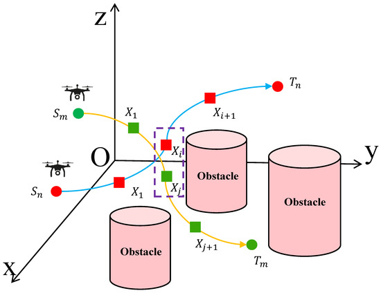
Figure 1.
Potential collision between two UAVs.
Specifically, a potential collision condition is satisfied when the Euclidean distance between UAV and UAV at any time step is smaller than a predefined safety distance, as defined in Equation (17).
where and represent the respective positions of the two points in the 3D space. Then the time difference at those points must also be checked using Equation (18).
If both conditions are met, and are considered to have a potential collision risk at that point, which is counted as a collision event. To avoid such events, a collision penalty term is added to the objective function, guiding the optimization process to steer clear of risky flight conflicts. The total collision check among UAVs is shown in Algorithm 1 and calculated by Equation (19).
where is the total number of collisions along the path. The coefficient 1000 is chosen to enforce safety while still allowing the algorithm to explore feasible paths. This balance ensures that the heuristic search mechanism can consider alternative routes, maintaining a trade-off between collision avoidance and solution space exploration.
| Algorithm 1: Collision check among UAVs |
 |
4. Reinforcement-Learning-Driven Multi-Strategy Continuous Ant Colony Optimization
This section presents the core algorithmic framework and the enhancements proposed in this paper. First, Section 4.1 introduces the standard continuous ant colony optimization (ACOR), which serves as the foundation for the proposed approach. Section 4.2 then reviews the basic principles of the Q-learning algorithm, highlighting its key components such as the state set, the action set, and the reward mechanism. Building upon these foundations, Section 4.3 proposes a novel reinforcement-learning-driven multi-strategy continuous ant colony optimization (QMSR-ACOR). This enhanced approach integrates multiple construction and walk strategies, a waypoint repair mechanism with elite selection, and a Q-learning-based strategy selection module to improve performance in complex continuous optimization tasks.
4.1. Standard Continuous Ant Colony Optimization
Socha et al. [13] extended ant colony optimization to continuous problems with ACOR, which uses probabilistic modeling to sample new solutions from continuous distributions, unlike discrete ACO finite selections.
Let us consider a general continuous optimization problem defined as follows in Equation (20).
where D be the continuous search space and the objective function to minimize. ACOR maintains an archive of elite k solutions , sorted by their objective values. Each solution receives a weight derived from a Gaussian function capturing its quality, as defined in Equation (21).
where l regulates the rate of weight decay: the smaller l concentrates the search for the optimal solutions, while the larger l encourages a wider exploration.
Next, the selection probability is derived by normalizing its weight, as given in Equation (22).
Then, ACOR randomly selects a guiding solution based on the probabilities and generates a new candidate by sampling each dimension from a Gaussian distribution. The mean is the value of the guide solution for that dimension and the standard deviation is based on the average distance to other solutions in the archive.
Specifically, a new solution is sampled as shown in Equation (23).
where is the component of the guiding solution in dimension d and the parameter controls convergence: larger means a wider search, while smaller means faster convergence but higher risk of premature stagnation.
4.2. Q-Learning Framework and Components
This section briefly reviews the basic Q-learning framework and presents its key components, including the state set, the action set, and the reward mechanism.
4.2.1. Q-Learning Framework
Q-learning is a model-free reinforcement learning algorithm that learns optimal policies in Markov Decision Processes (MDPs) by interacting with the environment, and has been widely applied in various fields [39,40,41]. Update action value (Q) functions using immediate rewards and state transitions, gradually converging to an optimal policy. During the learning process, the agent observes states, takes actions, and receives rewards that guide future decisions. A well-designed reward function is crucial: positive rewards reinforce good actions, while negative rewards discourage poor ones.
Q-learning balances exploration and exploitation: first exploring more to learn the environment, then exploiting the learned knowledge to improve performance. Its core update rule is defined as shown in Equation (25).
where denotes the current state, is the action taken in that state, is the immediate reward received after performing the action, and is the resulting state. The parameter controls how much new information updates the Q value, and is the discount factor that weighs immediate versus future rewards.
4.2.2. State Set
In multi-UAV path planning, the fitness function measures the quality of the solution. To better represent the search status of the population, we include both the average fitness and the current best fitness in the state design. The formulas are calculated using Equations (26)–(28).
where is the fitness of the ith solution in generation t, and is its fitness in the initial generation. and are the best fitness values in generations t and 1, respectively. Consequently, and represent the normalized performance at the population level and the individual level, while reflects the general state of the search. The state is discretized into four intervals with a width of 0.1. For example, if , then .
4.2.3. Action Set
The action set includes eight combinations made up of four constructor selection strategies and two walk strategies. These combinations represent different ways to build and explore solutions. Detailed explanations of each method and strategy will be provided in Section 4.3. The reinforcement learning agent dynamically selects among these combinations to adaptively optimize both construction and exploration, thereby improving search efficiency and solution quality.
In our Q-learning implementation, the action set consists of eight distinct actions, formed by combining four constructor selection strategies with two walk strategies. In the code, these actions are represented as an indexed list, where each index corresponds to a unique combination.
During the first half of the iterations, the agent selects actions randomly to encourage exploration. In the second half, it follows a greedy policy to exploit the learned knowledge. Each selected action determines:
- (1)
- Constructor selection strategy—guides how the partial solution is expanded.
- (2)
- Walk strategy—defines how the partial solution is extended or mutated to generate a new solution.
After executing the chosen action, the agent observes the resulting state and receives a reward. The Q-table is then updated according to the standard Q-learning update rule. This design allows the agent to balance exploration of alternative paths with exploitation of high-reward strategies.
4.2.4. Reward Mechanism
The reward function is based on the changes in the average fitness and the best fitness of the population between consecutive generations, guiding the agent to learn the optimal combination of strategies. The reward is calculated using Equation (29).
where measures the improvement of the best individual and evaluates the overall improvement of the population.
4.3. Reinforcement-Learning-Driven Multi-Strategy Continuous Ant Colony Optimization
In order to improve the effectiveness of ACOR for complex continuous optimization problems, this paper proposes a reinforcement-learning-driven multi-strategy continuous ant colony optimization (QMSR-ACOR). Specifically, we design four new constructor strategies, integrate two walk strategies from existing studies, and adopt a waypoint repair strategy that incorporates the proposed elite selection mechanism. Finally, we apply reinforcement learning to adaptively select the best combination of strategies.
4.3.1. Constructor Selection Strategies
In this section, we introduce four solution construction strategies.
- (1)
- Hybrid strategy mean-guided single-individual constructorIn high-dimensional and complex optimization problems, guiding vectors generated by a single selection strategy often fails to balance search diversity and solution quality. To overcome this, we propose a hybrid strategy mean-guided constructor (HMGSC). It simultaneously applies tournament selection, roulette wheel selection, and random selection to choose one individual from each, and generates the guiding vector by averaging these three individuals, as shown in Equation (32).where , , and are the individuals selected by tournament, roulette wheel, and random selection, respectively. After obtaining the guiding vector , the constructor further generates a new solution using a walk strategy, as given in Equation (33).In this mechanism, tournament selection focuses on high-quality individuals to strengthen local exploitation. Roulette wheel selection introduces a chance to select weaker individuals, preserving population diversity. Random selection increases the search’s jumpiness, enhancing global exploration. By averaging individuals from these three strategies, the method reduces the bias of any single selection approach. The pseudo code of HMGSC is presented in Algorithm 2.
Algorithm 2: Solution construction in HMGSC 
- (2)
- Adaptive differential-guided single-individual constructorTo better balance global exploration and local exploitation, we design an adaptive differential-guided single constructor (ADGSC). It extends the differential evolution (DE) strategy and incorporates a diversity-driven mechanism to adaptively adjust the perturbation strength, improving both solution quality and adaptability. In ADGSC, the guiding vector is generated using two individuals, and , selected from the archive by roulette wheel selection, as given in Equation (34).where is a perturbation factor that controls the step size of the differential vector. Instead of using a fixed value, ADGSC adaptively sets based on a normal distribution with a mean of 0.5 and a standard deviation determined by the current population diversity D (see Equations (35) and (36)).The diversity indicator D can be calculated by Equation (37).where denotes the value of the ith individual in the jth dimension, N is the population size, and n is the number of decision variables. Once the guiding vector is obtained, a new solution is generated using a walk strategy by Equation (33).This mechanism increases perturbation when diversity is high to enhance global exploration, and reduces it when diversity is low to improve local exploitation. It helps maintain a dynamic balance between search efficiency and solution quality. The pseudo code of ADGSC is shown in Algorithm 3.
Algorithm 3: Solution construction in ADGSC 
- (3)
- Adaptive differential-guided multi-individual constructorTo improve diversity, stability, and solution quality at different stages, we propose an adaptive differential-guided multi-individual constructor (ADGMC), building on ADGSC. Unlike ADGSC, which creates one guiding vector, ADGMC generates multiple guiding vectors and candidate solutions in parallel, enabling a more robust and multidirectional search. Specifically, in each construction phase, ADGMC generates three guiding vectors , , and , each representing a distinct search direction:First, the convergence-guided vector is constructed using the current best individual and a randomly selected individual from the population, as given in Equation (38).Second, the diversity-guided vector is generated by selecting two individuals, and , from the population using roulette wheel selection, as given in Equation (39).Third, the exploration-guided vector is constructed from two randomly selected individuals, and , from the population, as given in Equation (40).All guiding vectors share the same adaptive mechanism for determining the perturbation factor , which can be computed as (26). Finally, the three guiding vectors are used in a random walk strategy to generate three candidate solutions , , and , as given in Equation (41).By integrating convergence, diversity, and exploration vectors, ADGMC achieves a balanced trade-off between local exploitation and global exploration, thereby enhancing the comprehensiveness and robustness of the solution construction process. The pseudo code of ADGMC is shown in Algorithm 4.
Algorithm 4: Solution construction in ADGMC 
- (4)
- Elite genetic multi-individual constructorBased on the “selection–recombination” idea in genetic algorithms, we design the elite genetic multi-individual constructor (EGMC). It uses tournament selection to improve robustness and accelerate convergence by promoting high-quality individuals. Compared to roulette or random selection, tournament selection relies on local competition, making it more effective in complex or dynamic environments. During each construction cycle, EGMC combines elite guidance and tournament selection to generate three guiding vectors , , and , each responsible for directing the search in different directions. The specific construction methods are as follows.First, the convergence-guided vector is constructed using the current best individual and a randomly selected individual , as given in Equation (42).Second and third, the competitive-guided vectors and are generated using individuals , , , and selected by tournament selection. Each pair of relatively superior individuals is used to construct one guiding vector, as given in Equations (43) and (44).These vectors emphasize the genetic propagation of high-quality individuals through local competition, promoting effective exploration of elite regions while avoiding excessive reliance on the global best individual. The pseudo code of EGMC is shown in Algorithm 5.
Algorithm 5: Solution construction in EGMC 
4.3.2. Random Walk Strategy
In ACOR, new solutions are sampled using a Gaussian distribution, leading to small-step random walks similar to Brownian motion. This often limits exploration and increases the risk of premature convergence, especially in later stages. To address this, others introduce the Lévy flight [14], a stochastic process with a heavy-tailed power law distribution, defined as . Unlike Gaussian walks, Lévy flight allows for occasional long jumps, enhancing global exploration, and helping the algorithm escape local optima. Its effectiveness has been demonstrated in metaheuristics such as DE [44] and PSO [45]. The new solution is generated by Equation (45).
where is the step length in the Lévy flight.
4.3.3. Elite Waypoint Repair Strategy
In path planning, obstacles and constraints divide the search space into feasible and infeasible regions. The generated waypoints may fall within infeasible areas, making the path invalid. To simplify correcting these invalid points, we adopt a waypoint repair mechanism [16], enhanced with an elite repair strategy that selectively repairs only part of the population to improve computational efficiency.
In Figure 2, the first shows two UAVs ( and ) starting at different points with initial paths crossing cylindrical obstacles. These initial trajectories are generated without considering obstacle constraints, resulting in infeasible segments where the UAVs would collide with obstacles. The second one provides a top view of the path-obstacle intersections. Once these points are identified as infeasible, a two-step relocation strategy is applied to move them to feasible locations nearby.
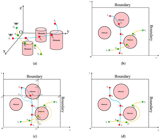
Figure 2.
Elite waypoint repair strategy. (a) 3D view. (b) Initial paths. (c) Repair process. (d) Repaired paths.
- Move the waypoint along the x-axis to any position within a feasible interval.
- Move the waypoint along the y-axis to any position within a feasible interval.
Specifically, the third figure shows that in is shifted along the x-axis to within intervals and . in is moved randomly along the y axis to within the intervals , , and .
Finally, the fourth figure shows the outcome of the repair strategy. After the relocation of infeasible waypoints, both the original and repaired paths are reconnected using smooth curved segments, ensuring that the resulting trajectories are not only collision-free, but also continuous and feasible for UAV navigation. This process improves the overall path quality and reliability of UAV operations in complex environments with dense obstacles. The pseudo code is shown in Algorithm 6.
| Algorithm 6: Elite waypoint repair strategy |
 |
4.3.4. Reinforcement-Learning-Driven Multi-Strategy Continuous Ant Colony Optimization for Path Planning
This proposed algorithm is built on the Q-learning framework, treating the population of ACOR as a reinforcement learning agent. During multi-UAV path planning, it adaptively optimizes solutions by selecting among multiple construction strategies and walk strategies. Specifically, the action set consists of eight combinations of strategies formed by pairing four construction strategies of solutions with two walking strategies: HMGSC + Gaussian Mutation, ADGSC + Gaussian Mutation, ADGMC + Gaussian Mutation, EGMC + Gaussian Mutation, HMGSC + Lévy Flight, ADGSC + Lévy Flight, ADGMC + Lévy Flight, and EGMC + Lévy Flight.
In early training, actions are randomly chosen to encourage exploration. Later, actions with the highest Q values are selected to exploit the learned experience. After each action, a reward is calculated based on changes in average and best fitness, and the Q values are updated accordingly. Then, the algorithm uniformly applies the elite waypoint repair strategy to correct invalid waypoints in the path, thereby improving the feasibility and robustness of the solution.
This learning mechanism helps the algorithm discover effective combinations of strategies, improving both search efficiency and path quality. It is especially suitable for complex, dynamic multi-UAV planning tasks. The pseudo code of QMSR-ACOR is shown in Algorithm 7.
| Algorithm 7: Pseudo-code of QMSR-ACOR |
 |
4.3.5. Time Complexity Analysis
To evaluate the efficiency of the proposed QMSR-ACOR in solving multi-UAV path planning problems, its time complexity is analyzed using big-O notation. In the algorithm, N denotes the population size, the number of waypoints, the number of obstacles, the number of UAVs, and the maximum number of iterations.
The algorithm consists of two main stages. The first stage is population initialization, which generates initial solutions for all UAVs. The time complexity of this stage is approximately , since each UAV in each individual requires generating waypoints.
The second stage is the iterative optimization process, repeated for each iteration, which includes four main components:
- (1)
- Solution construction and mutation: Each ant constructs a new solution based on selected strategies. The update of each coordinate using Gaussian mutation or Lévy flight has a complexity of .
- (2)
- Repair operation: For infeasible paths, each UAV’s trajectory is repaired considering obstacles, with a time complexity of .
- (3)
- Collision detection between UAVs: To avoid inter-UAV collisions, pairwise checks of all UAVs are performed for each path. The complexity is . Since is relatively small in practice, this term does not dominate the overall computation.
- (4)
- Fitness evaluation and global best update: Fitness evaluation involves computing path length, obstacle avoidance, and flight constraints for all UAVs (), while updating the global best solution requires sorting, with a complexity of .
The Q-learning component only involves table lookups and updates, which are negligible compared to the ACOR operations.
In summary, the total time complexity of QMSR-ACOR is:
When the population size N is much larger than the number of waypoints and obstacles , and the number of UAVs is small, the time complexity simplifies to:
which is consistent with the traditional ACOR family, indicating that the integration of Q-learning and multi-UAV collision checking does not significantly increase the overall computational burden.
5. Experimental Results and Analysis
5.1. Experimental Setting
To evaluate the performance and robustness of QMSR-ACOR in multi-UAV path planning, two groups of experiments were carried out in a simulated environment based on data from the digital elevation model (DEM) to replicate realistic terrains.
The first set tested the algorithm on different scales and complexities of the problem by varying the number of UAVs (2 to 6) and obstacles (5 to 12). Table A1 and Table A2 list UAV IDs, start/end points, and environmental details. Obstacles have a fixed height of 450 m. QMSR-ACOR was compared with six advanced algorithms: ACOSRAR [16], EEFO [34], HLOA [35], MACOR [14], SPSO [27], and ACOR [13]. Three problem dimensions, each with 8 cases, were independently tested 30 times. The parameter settings are shown in Table 1. Performance results and success rates are shown in Table 2, Table 3 and Table 4. Figure A1 shows the convergence curves (10D), and Figure A2 shows the optimal paths of QMSR-ACOR. The second set analyzed the internal mechanisms of QMSR-ACOR by evaluating different combinations of its eight component strategies to assess their contribution to the quality and optimization of the path.

Table 1.
Parameter settings in various comparison algorithms.
All experiments used consistent settings: 30 independent runs per case, with average and best path costs recorded. Statistical significance was verified using the Wilcoxon rank sum test (* marks 5% significance). The maximum number of iterations was 200, and the population size was 400. The best results are highlighted in bold.
5.2. The Comparison to Different Algorithms
This section presents a comprehensive comparison of QMSR-ACOR with seven baseline algorithms for test problems of increasing dimensionality: 10D, 20D and 30D. Evaluation metrics include success rate and average cost of the path, measured in eight benchmark cases for each dimension.
5.2.1. Comparison of Different Algorithms on 10D Cases
As shown in Table 2, we compared seven algorithms in eight test cases using the success rate and the average cost of the route as metrics in the 10D (30 parameters) path planning problem. In simpler cases (Case 1–Case 4), most algorithms (MACOR, SPSO, EEFO, HLOA, ACOR) achieved 100% success, indicating their effectiveness in low complexity scenarios. However, their performance dropped significantly in more complex cases (Case 5–Case 8), with some success rates falling to 0, highlighting weaknesses in solving high-dimensional constrained problems.
Table 2.
Comparison results on 10D cases.
Table 2.
Comparison results on 10D cases.
| Case | MACOR [14] | SPSO [27] | EEFO [34] | HLOA [35] | ACOR [13] | ACOSRAR [16] | QMSR-ACOR |
|---|---|---|---|---|---|---|---|
| 1 | 1598 ± 40 | 1783 ± 27 | 2134 ± 137 * | 2538 ± 121 * | 1776 ± 428 | 1521 ± 40 | 1690 ± 12 |
| 1.00 | 1.00 | 1.00 | 1.00 | 1.00 | 1.00 | 1.00 | |
| 2 | 2891 ± 158 | 3152 ± 132 * | 3836 ± 253 * | 4547 ± 182 * | 3385 ± 800 * | 2867 ± 246 | 2462 ± 16 |
| 1.00 | 1.00 | 1.00 | 1.00 | 1.00 | 1.00 | 1.00 | |
| 3 | 3240 ± 764 * | 3268 ± 134 * | 3249 ± 121 * | 4111 ± 237 * | 8219 ± 755 * | 3159 ± 415 * | 2516 ± 127 |
| 1.00 | 1.00 | 1.00 | 1.00 | 1.00 | 1.00 | 1.00 | |
| 4 | 6872 ± 782 * | 4721 ± 230 * | 5950 ± 490 * | 7004 ± 523 * | 18,135 ± 681 * | 5452 ± 367 * | 4080 ± 177 |
| 1.00 | 1.00 | 1.00 | 1.00 | 0.80 | 1.00 | 1.00 | |
| 5 | 18,215 ± 2434 * | 19,864 ± 1115 * | 18,585 ± 3105 * | 25,852 ± 2697 * | 26,309 ± 3693 * | 13,699 ± 1793 * | 8195 ± 516 |
| 0.80 | 0.60 | 0.80 | 0.20 | 0.20 | 1.00 | 1.00 | |
| 6 | 22,390 ± 3217 * | 32,955 ± 2510 * | 43,937 ± 2888 * | - | - | 22,350 ± 1699 * | 13,920 ± 1707 |
| 0.20 | 0.17 | 0.13 | 0.00 | 0.00 | 1.00 | 1.00 | |
| 7 | 21,360 ± 1849 * | 37,032 ± 1993 * | - | - | - | 46,927 ± 3259 * | 16,433 ± 2621 |
| 0.10 | 0.07 | 0.00 | 0.00 | 0.00 | 0.73 | 0.83 | |
| 8 | 44,396 ± 5232 * | - | - | - | - | 54,711 ± 7340 * | 23,717 ± 2786 |
| 0.07 | 0.00 | 0.00 | 0.00 | 0.00 | 0.57 | 0.70 |
* Indicates statistically worse results compared to the best.
In contrast, ACOSRAR and QMSR-ACOR maintained success rates above 50% in all cases, benefiting from their adaptive waypoint repair mechanism, which detects and corrects infeasible points during the search process. As the obstacle density increased, these two algorithms continued to find feasible paths, demonstrating strong robustness.
Between the two, QMSR-ACOR consistently achieved higher success rates, especially in highly constrained environments (e.g., Case 7 and Case 8). It also outperformed ACOSRAR in the cost of the path from Case 2 to Case 8, the performance gap expanding in more difficult problems. This advantage comes from its Q-learning-based constructor selection, which adaptively chooses among four strategies (HMGSC, ADGSC, ADGMC, EGMC), balancing exploration and exploitation. Combined with repair mechanisms, QMSR-ACOR ensures both feasibility and path quality under challenging conditions.
As shown in Figure A1, in the 10D path planning problem, the convergence curves from Case 1 to Case 8 show that QMSR-ACOR consistently achieves superior convergence performance across all scenarios. As environmental complexity increases, especially from Case 5 onwards due to more UAVs and denser obstacles, many algorithms tend to generate infeasible solutions in early iterations. The high penalty for obstacle collisions (up to 10,000) leads to a sharp increase in initial path costs, creating a noticeable ‘initial jump’ that hinders the quality of the initial solution and overall convergence. Although SPSO, EEFO, and HLOA can produce good initial paths and show strong early stage performance, their effectiveness drops significantly in complex environments. Some even fail to find feasible solutions entirely, indicating that they are better suited for simpler scenarios.
5.2.2. Comparison of Different Algorithms on 20D Cases
As shown in Table 3, when the dimension of the problem increases from 10D to 20D—corresponding to an increase in the number of parameters from 30 to 60—the search space and uncertainty of the path planning problem increase substantially. This significantly raises the difficulty of finding feasible paths and the path cost accordingly increases.
In high-dimensional scenarios, MACOR achieves 100% success in cases of low to medium complexity (Case 1–Case 4), but decreases dramatically in cases of higher dimension (Case 5–Case 8) to 0.57, 0.23, 0.06, and fails completely in Case 8, indicating that its search mechanism tends to fall into infeasible regions and lacks the ability to escape local optima. SPSO maintains 100% success in simple cases, but decreases rapidly to 0.13, 0.10, 0.00, and 0.00 in later cases, as its velocity–position update mechanism struggles to maintain direction in complex terrains and narrow feasible regions. EEFO and HLOA are theoretically designed to balance exploration and exploitation, but prove unstable under high-dimensional constraints, with path success rates below 0.2 or infeasible from Case 5 onwards, highlighting difficulties in generating feasible paths.
The original ACOR maintains reasonable performance in lower-dimensional problems but shows clear limitations under 20D conditions. From Case 4 onwards, its success rate drops drastically to 0.23, 0.00, 0.00, and 0.00, highlighting that its elite-solution-guided sampling strategy is prone to fall into “infeasibility traps” under high-dimensional constraints and lacks mechanisms for path correction and diversity enhancement.
In contrast, ACOSRAR and QMSR-ACOR exhibit strong stability and adaptability even as dimensionality increases. In particular, in the four most constrained scenarios (Case 5–Case 8), both algorithms maintain high success rates. Among them, QMSR-ACOR continues to demonstrate a significant advantage in path cost due to its Q-learning-based constructor selection mechanism and adaptive waypoint repair strategy, achieving both robustness and high quality of the solution under complex constraints.
Table 3.
Comparison results on 20D cases.
Table 3.
Comparison results on 20D cases.
| Case | MACOR [14] | SPSO [27] | EEFO [34] | HLOA [35] | ACOR [13] | ACOSRAR [16] | QMSR-ACOR |
|---|---|---|---|---|---|---|---|
| 1 | 2922 ± 78 * | 2511 ± 35 | 2790 ± 260 * | 2556 ± 117 | 2482 ± 211 | 1942 ± 155 | 2887 ± 90 |
| 1.00 | 1.00 | 1.00 | 1.00 | 1.00 | 1.00 | 1.00 | |
| 2 | 5483 ± 311 * | 4868 ± 524 * | 5489 ± 353 * | 6671 ± 416 * | 5915 ± 122 * | 5250 ± 124 | 4804 ± 745 |
| 1.00 | 1.00 | 1.00 | 1.00 | 1.00 | 1.00 | 1.00 | |
| 3 | 7198 ± 866 * | 6019 ± 541 * | 7815 ± 748 * | 9015 ± 541 * | 9944 ± 873 * | 5627 ± 545 * | 4746 ± 610 |
| 1.00 | 1.00 | 1.00 | 1.00 | 1.00 | 1.00 | 1.00 | |
| 4 | 10,518 ± 947 * | 10,124 ± 1454 * | 13,594 ± 2132 * | 15,597 ± 2654 * | 18,310 ± 2248 * | 10,758 ± 800 * | 8138 ± 854 |
| 1.00 | 0.77 | 0.87 | 0.77 | 0.60 | 1.00 | 1.00 | |
| 5 | 22,795 ± 4562 * | 23,261 ± 3422 * | 25,323 ± 4100 * | 29,554 ± 3337 * | 33,710 ± 2849 * | 17,045 ± 2113 * | 12,125 ± 1022 |
| 0.57 | 0.13 | 0.17 | 0.06 | 0.23 | 0.93 | 0.93 | |
| 6 | 28,583 ± 3798 * | 36,487 ± 3091 * | 50,010 ± 4587 * | - | - | 25,714 ± 5571 * | 19,590 ± 1636 |
| 0.23 | 0.10 | 0.10 | 0.00 | 0.00 | 0.80 | 0.87 | |
| 7 | 29,749 ± 6523 * | - | - | - | - | 50,397 ± 4440 * | 22,848 ± 2472 |
| 0.06 | 0.00 | 0.00 | 0.00 | 0.00 | 0.53 | 0.63 | |
| 8 | - | - | - | - | - | 59430 ± 5388 * | 29,880 ± 2261 |
| 0.00 | 0.00 | 0.00 | 0.00 | 0.00 | 0.53 | 0.53 |
* Indicates statistically worse results compared to the best.
5.2.3. Comparison of Different Algorithms on 30D Cases
As shown in Table 4, in the 30D high-dimensional path planning problem, although MACOR, SPSO, EEFO, HLOA, and ACOR all maintained a success rate 100% in Case 1 and Case 2, performance degradation became apparent from Case 3. In particular, the success rates of HLOA and ACOR began to decline, and by Case 4, most algorithms failed to generate feasible paths, with the success rates dropping to zero. This indicates that these algorithms struggle to remain stable in complex high-dimensional scenarios. In particular, HLOA and ACOR completely failed after Case 4, revealing a weak adaptability under such conditions.
In contrast, ACOSRAR performs relatively stably in Case 1 to Case 5, with a success rate consistently remaining above 0.5. Although its success rate gradually decreased in Cases 6–8, it still outperformed most other algorithms, indicating a certain degree of robustness. However, its average path cost in high complexity scenarios (Cases 6–8) remained relatively high, suggesting that there is room for improvement in search precision.
The most notable performance was observed with QMSR-ACOR. Using the dynamic guidance of a Q-learning-based constructor selection mechanism, it can intelligently choose the optimal construction strategy during path generation. As a result, QMSR-ACOR consistently maintained a high success rate in all test cases (the lowest being 0.33), showing strong feasibility seeking capability even under complex, high-dimensional constraints. Furthermore, its average cost in Cases 3–8 was significantly lower than that of other algorithms, demonstrating superior global search capabilities and effective control over path quality. Therefore, QMSR-ACOR demonstrates outstanding stability and efficiency in high-dimensional path planning problems, significantly outperforming both traditional and improved algorithms. It proves to be an effective solution to tackle path planning in large-scale, complex environments.
Table 4.
Comparison results on 30D cases.
Table 4.
Comparison results on 30D cases.
| Case | MACOR [14] | SPSO [27] | EEFO [34] | HLOA [35] | ACOR [13] | ACOSRAR [16] | QMSR-ACOR |
|---|---|---|---|---|---|---|---|
| 1 | 4001 ± 155 * | 4716 ± 415 * | 5201 ± 316 * | 5038 ± 279 * | 4998 ± 407 * | 2388 ± 299 | 4499 ± 372 * |
| 1.00 | 1.00 | 1.00 | 1.00 | 1.00 | 1.00 | 1.00 | |
| 2 | 7186 ± 344 | 8296 ± 397 * | 9914 ± 518 * | 8727 ± 534 * | 9252 ± 3619 * | 8192 ± 537 | 6813 ± 470 |
| 1.00 | 1.00 | 1.00 | 1.00 | 1.00 | 1.00 | 1.00 | |
| 3 | 13,857 ± 2156 * | 9944 ± 990 * | 11,209 ± 955 * | 13,550 ± 2210 * | 15,380 ± 2437 * | 9362 ± 838 * | 8824 ± 525 |
| 1.00 | 1.00 | 1.00 | 0.87 | 0.80 | 1.00 | 1.00 | |
| 4 | 22,656 ± 6100 * | 22,470 ± 1901 * | 21,594 ± 1219 * | - | - | 16,398 ± 1215 * | 15,346 ± 572 |
| 0.80 | 0.63 | 0.50 | 0.00 | 0.00 | 0.93 | 1.00 | |
| 5 | 33,925 ± 5793 * | - | - | - | - | 22,967 ± 1138 * | 19,567 ± 893 |
| 0.57 | 0.00 | 0.00 | 0.00 | 0.00 | 0.57 | 0.90 | |
| 6 | - | - | - | - | - | 30,988 ± 1825 * | 24,580 ± 1292 |
| 0.00 | 0.00 | 0.00 | 0.00 | 0.00 | 0.30 | 0.40 | |
| 7 | - | - | - | - | - | 53,001 ± 4107 * | 27,111 ± 2965 |
| 0.00 | 0.00 | 0.00 | 0.00 | 0.00 | 0.33 | 0.33 | |
| 8 | - | - | - | - | - | 59,999 ± 5065 * | 34,304 ± 3389 |
| 0.00 | 0.00 | 0.00 | 0.00 | 0.00 | 0.20 | 0.33 |
* Indicates statistically worse results compared to the best.
In general, the results confirm that QMSR-ACOR provides robust and reliable convergence across varying complexities, thanks to its Q-learning-based strategy selection and elite waypoint repair mechanism.
5.2.4. Computational Time
To evaluate the computational complexity of the algorithms, we measured the time each algorithm required to solve the 10D UAV path planning problems. Specifically, we recorded the total execution time for each algorithm using 10,000 fitness evaluations and averaged the results over 30 independent runs. The results are summarized in Table 5.
Table 5.
Computational time on 10D cases.
From Table 5, several observations can be made. First, with the increase in case number, the execution time of all algorithms shows a rising trend, which is mainly because more UAVs and obstacles lead to larger problem scales and higher computational burdens. Second, SPSO, EEFO, and HLOA generally exhibit lower execution times compared to other algorithms, benefiting from their relatively simple update mechanisms. Third, the execution times of MACOR, ACOR, ACOSRAR, and the proposed QMSR-ACOR are higher, since constructing new solutions requires additional sampling and ranking operations. Among them, QMSR-ACOR achieves computational times comparable to MACOR and ACOSRAR, indicating that the incorporation of the proposed strategies does not lead to a significant increase in computational cost. Finally, although SPSO runs faster in most cases, it sacrifices solution quality in complex UAV path planning scenarios, while QMSR-ACOR strikes a better balance between execution time and solution quality, making it a more competitive choice in practice.
5.3. The Impacts of Various Strategies
This study designed eight strategies by combining four constructor strategies and two walk strategies. They are: HMGSC + Gaussian Mutation, ADGSC + Gaussian Mutation, ADGMC + Gaussian Mutation, EGMC + Gaussian Mutation, HMGSC + Lévy Flight, ADGSC + Lévy Flight, ADGMC + Lévy Flight, and EGMC + Lévy Flight correspond to Strategies 1–8, respectively. The results are summarized in Table 6 and the convergence curves of different strategies are illustrated in Figure A3.
Table 6.
Ablation study results of eight strategy combinations compared with QMSR-ACOR.
As shown in Table 6 and Figure A3, we can conclude that the type of constructor significantly affects the algorithm performance. Among the eight strategies, those that used ADGSC (Strategies 2 and 6) and EGMC (Strategies 4 and 8) consistently achieved lower path costs, especially in complex scenarios (Cases 4–8), indicating strong search ability and better adaptability. In contrast, HMGSC (Strategies 1 and 5) and ADGMC (Strategy 7) were unable to find feasible routes in highly constrained cases (Cases 5–8), showing weaker robustness.
Regarding walk strategies, the Gaussian mutation (Strategies 1–4) generally performed better than the Lévy flight (Strategies 5–8). This is particularly evident when comparing the same constructor under different walk strategies, such as Strategy 2 vs. 6 and Strategy 4 vs. 8. Although Lévy flight offers strong global search ability, applying it from the early stages introduces high variability, which may disrupt promising individuals and reduce convergence stability. Thus, Lévy flight is more effective when applied in later search stages to help escape local optima, rather than throughout the entire process. In particular, Strategies 5, 7, and 8 sometimes escaped local optima, but their overall path quality and stability were inferior to Strategies 1–4. This suggests that the Gaussian mutation provides better guidance and reliability in most scenarios.
In general, the combination of ADGSC or EGMC with Gaussian mutation (Strategies 2 and 4) delivered the best performance in terms of both convergence speed and solution quality. Furthermore, QMSR-ACOR achieved the lowest path cost in most cases, maintaining high robustness even under complex conditions (e.g., Cases 6–8). Its Q-learning mechanism enables dynamic selection of constructor–walk combinations based on current search states, balancing exploration and exploitation. This adaptability helps prevent premature convergence and improves overall path planning performance.
6. Conclusions
This paper proposes a reinforcement-learning-driven multi-strategy continuous ant colony optimization, namely QMSR-ACOR, to address the complex problem of multi-UAV path planning in 3D continuous environments. The proposed method incorporates a Q-learning-based strategy selector that adaptively chooses among eight path generation strategies to improve environmental adaptability. In addition, an elite waypoint repair mechanism is introduced to improve obstacle avoidance efficiency and reduce the generation of infeasible paths. Experimental results demonstrate that QMSR-ACOR not only achieves superior performance in path quality and computational efficiency, but also exhibits strong generalization across different scenarios compared to existing state-of-the-art algorithms.
The main contributions of this work are threefold: (1) modeling the multi-UAV path planning problem in 3D continuous space with realistic collaborative constraints; (2) integrating reinforcement learning into the strategy selection process to improve adaptability and robustness; and (3) enhancing search efficiency via an elite waypoint repair mechanism that guides UAVs away from invalid regions.
Although the proposed method shows promising results, there are still several directions worth exploring in future work. First, the current model assumes static obstacles and prior knowledge of the environment. In future research, incorporating online learning and real-time perception to handle partially known or dynamic environments will be critical. Second, communication and coordination strategies among UAVs can be further optimized to enhance collaborative efficiency under stricter constraints. Third, we plan to extend our study beyond simulations by conducting small-scale hardware experiments with multiple UAVs, which will provide further validation of the proposed method in real-world scenarios. Overall, QMSR-ACOR provides a viable and extensible solution to multi-UAV path planning in challenging environments and lays the foundation for further exploration into intelligent swarm-based navigation systems.
Author Contributions
Y.W.: Conceptualization, Investigation, Methodology, Software, Writing—original draft, Writing—review and editing; J.L.: Investigation, Methodology, Software, Writing—original draft, Writing—review and editing; Y.Q.: Writing—original draft, Writing—review and editing; W.Y.: Conceptualization, Supervision, Writing—review and editing, Funding acquisition. All authors have read and agreed to the published version of the manuscript.
Funding
This work is supported by Shenzhen Higher Education Support Plan (Project No. 20231120174835002) and National Natural Science Foundation of China (Project No. 72401202).
Data Availability Statement
The original contributions presented in this study are included in the article. Further inquiries can be directed to the corresponding author.
Conflicts of Interest
The authors declare no conflicts of interest.
Appendix A
Table A1.
Environment information for UAV path planning cases.
Table A1.
Environment information for UAV path planning cases.
| Case | Number of UAVs | Number of Obstacles | UAV ID | Start Point | End Point |
|---|---|---|---|---|---|
| 1 | 2 | 5 | UAV1 | (200, 200, 120) | (850, 750, 150) |
| UAV2 | (220, 400, 120) | (800, 200, 150) | |||
| 2 | 3 | 5 | UAV1 | (200, 200, 120) | (850, 750, 150) |
| UAV2 | (220, 400, 120) | (800, 200, 150) | |||
| UAV3 | (100, 500, 150) | (900, 600, 160) | |||
| 3 | 3 | 7 | UAV1 | (200, 200, 120) | (850, 750, 150) |
| UAV2 | (220, 400, 120) | (800, 200, 150) | |||
| UAV3 | (100, 500, 150) | (900, 600, 160) | |||
| 4 | 4 | 7 | UAV1 | (200, 200, 120) | (850, 750, 150) |
| UAV2 | (220, 400, 120) | (800, 200, 150) | |||
| UAV3 | (100, 500, 150) | (900, 600, 160) | |||
| UAV4 | (300, 800, 130) | (900, 400, 160) | |||
| 5 | 4 | 9 | UAV1 | (100, 300, 120) | (900, 700, 150) |
| UAV2 | (200, 200, 120) | (950, 600, 150) | |||
| UAV3 | (200, 700, 150) | (850, 100, 160) | |||
| UAV4 | (300, 800, 130) | (900, 200, 160) | |||
| 6 | 5 | 9 | UAV1 | (100, 300, 120) | (900, 700, 150) |
| UAV2 | (200, 200, 120) | (950, 600, 150) | |||
| UAV3 | (200, 700, 150) | (850, 100, 160) | |||
| UAV4 | (300, 800, 130) | (900, 200, 160) | |||
| UAV5 | (900, 400, 130) | (200, 100, 150) | |||
| 7 | 5 | 12 | UAV1 | (100, 300, 120) | (900, 700, 150) |
| UAV2 | (200, 200, 120) | (950, 600, 150) | |||
| UAV3 | (200, 700, 150) | (850, 100, 160) | |||
| UAV4 | (300, 800, 130) | (900, 200, 160) | |||
| UAV5 | (900, 400, 130) | (200, 100, 150) | |||
| 8 | 6 | 12 | UAV1 | (100, 300, 120) | (900, 700, 150) |
| UAV2 | (200, 200, 120) | (950, 600, 150) | |||
| UAV3 | (200, 700, 150) | (850, 100, 160) | |||
| UAV4 | (300, 800, 130) | (900, 200, 160) | |||
| UAV5 | (900, 400, 130) | (200, 100, 150) | |||
| UAV6 | (700, 800, 150) | (150, 500, 170) |
Table A2.
Obstacle information for each case.
Table A2.
Obstacle information for each case.
| Case | Obstacle Information |
|---|---|
| 1, 2 | O1(380,500,10,80); O2(720,320,10,80); O3(550,390,10,80); O4(740,560,10,60); O5(350,200,10,80) |
| 3, 4 | O1(380,500,10,80); O2(720,320,10,80); O3(550,390,10,80); O4(740,560,10,60); O5(350,200,10,80); O6(600,700,10,60); O7(550,200,10,60) |
| 5, 6 | O1(380,500,10,80); O2(720,320,10,80); O3(550,390,10,80); O4(740,560,10,60); O5(350,200,10,80); O6(600,700,10,60); O7(550,200,10,60); O8(550,550,0,50); O9(250,400,0,50) |
| 7, 8 | O1(380,500,10,80); O2(720,320,10,80); O3(550,390,10,80); O4(740,560,10,60); O5(350,200,10,80); O6(600,700,10,60); O7(550,200,10,60); O8(550,550,0,50); O9(250,400,0,50); O10(450,800,50,50); O11(750,150,10,30); O12(200,600,10,50) |
Appendix B
Appendix B.1

Figure A1.
The convergence graphs of comparison algorithms for 10D cases. (a) Case 1. (b) Case 2. (c) Case 3. (d) Case 4. (e) Case 5. (f) Case 6. (g) Case 7. (h) Case 8.
Figure A1.
The convergence graphs of comparison algorithms for 10D cases. (a) Case 1. (b) Case 2. (c) Case 3. (d) Case 4. (e) Case 5. (f) Case 6. (g) Case 7. (h) Case 8.

Appendix B.2

Figure A2.
The best generated 3D view paths in 10D cases by QMSR-ACOR. (a) Case 1. (b) Case 2. (c) Case 3. (d) Case 4. (e) Case 5. (f) Case 6. (g) Case 7. (h) Case 8.
Figure A2.
The best generated 3D view paths in 10D cases by QMSR-ACOR. (a) Case 1. (b) Case 2. (c) Case 3. (d) Case 4. (e) Case 5. (f) Case 6. (g) Case 7. (h) Case 8.

Appendix B.3

Figure A3.
The convergence graphs between QMSR-ACOR and single-strategy variants. (a) Case 1. (b) Case 2. (c) Case 3. (d) Case 4. (e) Case 5. (f) Case 6. (g) Case 7. (h) Case 8.
Figure A3.
The convergence graphs between QMSR-ACOR and single-strategy variants. (a) Case 1. (b) Case 2. (c) Case 3. (d) Case 4. (e) Case 5. (f) Case 6. (g) Case 7. (h) Case 8.

References
- Tolentino, V.; Ortega Lucero, A.; Koerting, F.; Savinova, E.; Hildebrand, J.C.; Micklethwaite, S. Drone-Based VNIR–SWIR Hyperspectral Imaging for Environmental Monitoring of a Uranium Legacy Mine Site. Drones 2025, 9, 313. [Google Scholar] [CrossRef]
- Mohamed, A.; Mohamed, M. Unmanned Aerial Vehicles in Last-Mile Parcel Delivery: A State-of-the-Art Review. Drones 2025, 9, 413. [Google Scholar] [CrossRef]
- Galindo Mendoza, M.G.; Cárdenas Tristán, A.; Pérez Medina, P.; Schwentesius Rindermann, R.; Rivas García, T.; Contreras Servín, C.; Reyes Cárdenas, O. Agroecological Alternatives for Substitution of Glyphosate in Orange Plantations (Citrus sinensis) Using GIS and UAVs. Drones 2025, 9, 398. [Google Scholar] [CrossRef]
- Shakhatreh, H.; Sawalmeh, A.H.; Al-Fuqaha, A.; Dou, Z.; Almaita, E.; Khalil, I.; Othman, N.S.; Khreishah, A.; Guizani, M. Unmanned Aerial Vehicles (UAVs): A Survey on Civil Applications and Key Research Challenges. IEEE Access 2019, 7, 48572–48634. [Google Scholar] [CrossRef]
- Wang, F.; Gao, M.; Qin, J.; Peng, Z.; Zheng, W. Adaptive Super-Twisting Sliding Mode Observer Based Positionless Direct Torque Control Strategy for PMSM. Nondestruct. Test. Eval. 2025, 1–24. [Google Scholar] [CrossRef]
- Chen, H.; Lan, Y.; Fritz, B.K.; Hoffmann, W.C.; Liu, S. Review of Agricultural Spraying Technologies for Plant Protection Using Unmanned Aerial Vehicle (UAV). Int. J. Agric. Biol. Eng. 2021, 14, 38–49. [Google Scholar] [CrossRef]
- Cui, J.Q.; Phang, S.K.; Ang, K.Z.Y.; Wang, F.; Dong, X.; Ke, Y.; Lai, S.; Li, K.; Li, X.; Lin, J.; et al. Search and Rescue Using Multiple Drones in Post-Disaster Situation. Unmanned Syst. 2016, 4, 83–96. [Google Scholar] [CrossRef]
- Luo, J.; Tian, Y.; Wang, Z. Research on Unmanned Aerial Vehicle Path Planning. Drones 2024, 8, 51. [Google Scholar] [CrossRef]
- Dorigo, M.; Stützle, T. The Ant Colony Optimization Metaheuristic: Algorithms, Applications, and Advances. In Handbook of Metaheuristics; Glover, F., Kochenberger, G.A., Eds.; Springer: Boston, MA, USA, 2003; pp. 250–285. [Google Scholar]
- Motamedi, A.; Mortazavi, M.; Sabzehparvar, M.; Duchon, F. Minimum time search using ant colony optimization for multiple fixed-wing UAVs in dynamic environments. Appl. Soft Comput. 2024, 165, 112025. [Google Scholar] [CrossRef]
- Cekmez, U.; Ozsiginan, M.; Sahingoz, O.K. Multi colony ant optimization for UAV path planning with obstacle avoidance. In Proceedings of the 2016 International Conference on Unmanned Aircraft Systems (ICUAS), Arlington, VA, USA, 7–10 June 2016; pp. 47–52. [Google Scholar]
- Li, Y.; Zhang, Z.; Sun, Q.; Huang, Y. An improved ant colony algorithm for multiple unmanned aerial vehicles route planning. J. Frankl. Inst. 2024, 361, 107060. [Google Scholar] [CrossRef]
- Socha, K.; Dorigo, M. Ant colony optimization for continuous domains. Eur. J. Oper. Res. 2008, 185, 1155–1173. [Google Scholar] [CrossRef]
- Liu, J.; Anavatti, S.; Garratt, M.; Abbass, H.A. Multi-operator continuous ant colony optimisation for real world problems. Swarm Evol. Comput. 2022, 69, 100984. [Google Scholar] [CrossRef]
- Wang, Y.; Chen, P.; Wu, Y.; Chen, W.; Tan, L. Modified Continuous Ant Colony Optimisation with Local Search for Multiple Unmanned Aerial Vehicle Path Planning. In Proceedings of the 2024 6th International Conference on Data-Driven Optimization of Complex Systems (DOCS), Hangzhou, China, 16–18 August 2024; pp. 557–564. [Google Scholar]
- Niu, B.; Wang, Y.; Liu, J.; Yue, G.X.-G. Path planning for unmanned aerial vehicles in complex environment based on an improved continuous ant colony optimisation. Comput. Electr. Eng. 2025, 123, 110034. [Google Scholar] [CrossRef]
- Dhulkefl, E.; Durdu, A.; Terzioğlu, H. Dijkstra Algorithm Using UAV Path Planning. Konya J. Eng. Sci. 2020, 8, 92–105. [Google Scholar] [CrossRef]
- Chen, J.; Li, M.; Yuan, Z.; Gu, Q. An Improved A* Algorithm for UAV Path Planning Problems. In Proceedings of the 2020 IEEE 4th Information Technology, Networking, Electronic and Automation Control Conference (ITNEC), Chongqing, China, 12–14 June 2020; pp. 958–962. [Google Scholar]
- Zhang, Z.; Jiang, J.; Wu, J.; Zhu, X. Efficient and Optimal Penetration Path Planning for Stealth Unmanned Aerial Vehicle Using Minimal Radar Cross-Section Tactics and Modified A-Star Algorithm. ISA Trans. 2023, 134, 42–57. [Google Scholar] [CrossRef] [PubMed]
- Liu, L.; Wang, X.; Yang, X.; Liu, H.; Li, J.; Wang, P. Path Planning Techniques for Mobile Robots: Review and Prospect. Expert Syst. Appl. 2023, 227, 120254. [Google Scholar] [CrossRef]
- Chen, X.; Chen, X. The UAV Dynamic Path Planning Algorithm Research Based on Voronoi Diagram. In Proceedings of the 26th Chinese Control and Decision Conference (CCDC), Changsha, China, 31 May–2 June 2014; pp. 1069–1071. [Google Scholar]
- Contreras, J.D.; Martínez, F.H. Path Planning for Mobile Robots Based on Visibility Graphs and A* Algorithm. In Proceedings of the Seventh International Conference on Digital Image Processing (ICDIP 2015), San Diego, CA, USA, 27–30 July 2015; pp. 345–350. [Google Scholar]
- Ghambari, S.; Golabi, M.; Jourdan, L.; Lepagnot, J.; Idoumghar, L. UAV Path Planning Techniques: A Survey. RAIRO Oper. Res. 2024, 58, 2951–2989. [Google Scholar] [CrossRef]
- Fan, X.; Guo, Y.; Liu, H.; Wei, B.; Lyu, W. Improved Artificial Potential Field Method Applied for AUV Path Planning. Math. Probl. Eng. 2020, 2020, 6523158. [Google Scholar] [CrossRef]
- Pan, Z.; Zhang, C.; Xia, Y.; Xiong, H.; Shao, X. An Improved Artificial Potential Field Method for Path Planning and Formation Control of the Multi-UAV Systems. IEEE Trans. Circuits Syst. II Express Briefs 2021, 69, 1129–1133. [Google Scholar] [CrossRef]
- Cheng, C.; Sha, Q.; He, B.; Li, G. Path Planning and Obstacle Avoidance for AUV: A Review. Ocean Eng. 2021, 235, 109355. [Google Scholar] [CrossRef]
- Phung, M.D.; Ha, Q.P. Safety-Enhanced UAV Path Planning with Spherical Vector-Based Particle Swarm Optimization. Appl. Soft Comput. 2021, 107, 107376. [Google Scholar] [CrossRef]
- Huang, C.; Zhao, Y.; Zhang, M.; Yang, H. APSO: An A*-PSO Hybrid Algorithm for Mobile Robot Path Planning. IEEE Access 2023, 11, 43238–43256. [Google Scholar] [CrossRef]
- Yu, Z.; Si, Z.; Li, X.; Wang, D.; Song, H. A Novel Hybrid Particle Swarm Optimization Algorithm for Path Planning of UAVs. IEEE Internet Things J. 2022, 9, 22547–22558. [Google Scholar] [CrossRef]
- Tan, L.; Zhang, H.; Shi, J.; Liu, Y.; Yuan, T. A Robust Multiple Unmanned Aerial Vehicles 3D Path Planning Strategy via Improved Particle Swarm Optimization. Comput. Electr. Eng. 2023, 111, 108947. [Google Scholar] [CrossRef]
- Rosas-Carrillo, A.S.; Solís-Santomé, A.; Silva-Sánchez, C.; Camacho-Nieto, O. UAV Path Planning Using an Adaptive Strategy for the Particle Swarm Optimization Algorithm. Drones 2025, 9, 170. [Google Scholar] [CrossRef]
- Xu, C.; Duan, H.; Liu, F. Chaotic artificial bee colony approach to Uninhabited Combat Air Vehicle (UCAV) path planning. Aerosp. Sci. Technol. 2010, 14, 535–541. [Google Scholar] [CrossRef]
- Bhattacharjee, P.; Rakshit, P.; Goswami, I.; Konar, A.; Nagar, A.K. Multi-robot path-planning using artificial bee colony optimization algorithm. In Proceedings of the 2011 Third World Congress on Nature and Biologically Inspired Computing, Salamanca, Spain, 19–21 October 2011; pp. 219–224. [Google Scholar]
- Zhao, W.; Wang, L.; Zhang, Z.; Fan, H.; Zhang, J.; Mirjalili, S.; Khodadadi, N.; Cao, Q. Electric eel foraging optimization: A new bio-inspired optimizer for engineering applications. Expert Syst. Appl. 2024, 238, 122200. [Google Scholar] [CrossRef]
- Peraza-Vázquez, H.; Peña-Delgado, A.; Merino-Treviño, M.; Morales-Cepeda, A.B.; Sinha, N. A novel metaheuristic inspired by horned lizard defense tactics. Artif. Intell. Rev. 2024, 57, 59. [Google Scholar] [CrossRef]
- Li, G.; Liu, C.; Wu, L.; Xiao, W. A Mixing Algorithm of ACO and ABC for Solving Path Planning of Mobile Robot. Appl. Soft Comput. 2023, 148, 110868. [Google Scholar] [CrossRef]
- Lu, Y.; Da, C. Global and Local Path Planning of Robots Combining ACO and Dynamic Window Algorithm. Sci. Rep. 2025, 15, 9452. [Google Scholar] [CrossRef]
- Cai, Z.; Liu, J.; Xu, L.; Wang, J. Cooperative Path Planning Study of Distributed Multi-Mobile Robots Based on Optimised ACO Algorithm. Robot. Auton. Syst. 2024, 179, 104748. [Google Scholar] [CrossRef]
- Duan, Z.; Zhang, Y.; Wang, R.; Xu, Z.; Xiang, Z. A Q-Learning-Based Multi-Objective PSO Algorithm for Robot Path Planning on Rough Terrain. In Proceedings of the 2025 IEEE 14th Data Driven Control and Learning Systems (DDCLS), Guangzhou, China, 16–18 May 2025; pp. 123–128. [Google Scholar]
- Liu, Y.; Lu, H.; Cheng, S.; Shi, Y. An Adaptive Online Parameter Control Algorithm for Particle Swarm Optimization Based on Reinforcement Learning. In Proceedings of the 2019 IEEE Congress on Evolutionary Computation (CEC), Wellington, New Zealand, 10–13 June 2019; pp. 815–822. [Google Scholar]
- Wang, X.; Yao, H.; Mai, T.; Guo, S.; Liu, Y. Reinforcement learning-based particle swarm optimization for end-to-end traffic scheduling in TSN-5G networks. IEEE/ACM Trans. Netw. 2023, 31, 3254–3268. [Google Scholar] [CrossRef]
- Ekechi, C.C. Intelligent control of a Swarm of Unmanned Aerial Vehicles in Turbulent Environments Using Clustering-PPO Algorithm. Master’s Thesis, Tennessee Technological University, Cookeville, TN, USA, 2023. [Google Scholar]
- He, K.; Sun, L.; Hong, H.; Wang, N.; Xiang, X.; Lu, Z.; Cai, L. Target allocation for multiple UAVs via swarm intelligence simulation and DDPG reinforcement learning. Int. J. Model. Simul. Sci. Comput. 2025, 16, 450012. [Google Scholar] [CrossRef]
- Wang, W.-C.; Xu, L.; Chau, K.-W.; Liu, C.-J.; Ma, Q.; Xu, D.-M. Cε-LDE: A lightweight variant of differential evolution algorithm with combined ε constrained method and Lévy flight for constrained optimization problems. Expert Syst. Appl. 2023, 211, 118644. [Google Scholar] [CrossRef]
- Gao, Y.; Zhang, H.; Duan, Y.; Zhang, H. A novel hybrid PSO based on Lévy flight and wavelet mutation for global optimization. PLoS ONE 2023, 18, e0279572. [Google Scholar] [CrossRef]


Disclaimer/Publisher’s Note: The statements, opinions and data contained in all publications are solely those of the individual author(s) and contributor(s) and not of MDPI and/or the editor(s). MDPI and/or the editor(s) disclaim responsibility for any injury to people or property resulting from any ideas, methods, instructions or products referred to in the content. |
© 2025 by the authors. Licensee MDPI, Basel, Switzerland. This article is an open access article distributed under the terms and conditions of the Creative Commons Attribution (CC BY) license (https://creativecommons.org/licenses/by/4.0/).