SGGTSO: A Spherical Vector-Based Optimization Algorithm for 3D UAV Path Planning

Abstract

The application of 3D UAV path planning algorithms in smart cities and smart buildings can improve logistics efficiency, enhance emergency response capabilities as well as provide services such as indoor navigation, thus bringing more convenience and safety to people’s lives and work. The main idea of the 3D UAV path planning problem is how to plan to get an optimal flight path while ensuring that the UAV does not collide with obstacles during flight. This paper transforms the 3D UAV path planning problem into a multi-constrained optimization problem by formulating the path length cost function, the safety cost function, the flight altitude cost function and the smoothness cost function. This paper encodes each feasible flight path as a set of vectors consisting of magnitude, elevation and azimuth angles and searches for the optimal flight path in the configuration space by means of a metaheuristic algorithm. Subsequently, this paper proposes an improved tuna swarm optimization algorithm based on a sigmoid nonlinear weighting strategy, multi-subgroup Gaussian mutation operator and elite individual genetic strategy, called SGGTSO. Finally, the SGGTSO algorithm is compared with some other classical and novel metaheuristics in a 3D UAV path planning problem with nine different terrain scenarios and in the CEC2017 test function set. The comparison results show that the flight path planned by the SGGTSO algorithm significantly outperforms other comparison algorithms in nine different terrain scenarios, and the optimization performance of SGGTSO outperforms other comparison algorithms in 24 CEC2017 test functions.

1. Introduction

Unmanned aerial vehicles (UAVs) have attracted a lot of attention in recent years because of their small size, flexibility and adaptability to the environment. With the rapid development of the Internet of Things and computer technology, UAVs have been widely used in important fields such as communication [1], tracking [2], environmental monitoring [3], agricultural management [4], and disaster monitoring [5]. The 3D UAV path planning algorithm has important values and applications in smart cities and smart buildings, for example, UAVs can be applied for logistics distribution in smart cities, UAVs can be used for rapid response and rescue in disaster events or emergencies in cities and UAVs can provide indoor navigation services in large smart buildings. High-performance 3D UAV path planning algorithms can help UAVs plan the shortest distance and safest path, thus improving logistics efficiency, achieving rapid rescue and providing real-time guidance. When a UAV executes a mission independently, the environment it faces does not provide good feedback to the controller, so it is indispensable for the UAV to plan its own path to complete the mission successfully. Autonomous UAV path planning means that after determining the start and end points of the path, the UAV not only needs to find the shortest distance path, but also take into account altitude factors, fuel costs and safety factors, etc., and optimize the integrated cost function in compliance with the dynamical constraints [6].

In recent years, researchers have been conducting more and more useful explorations on the path planning problems for UAVs [7,8,9,10,11,12,13,14,15]. UAV path planning is a complex and multi-constrained optimization problem that requires comprehensive consideration of flight path length, fuel consumption, obstacle avoidance, and robustness. Li et al. proposed a flipping ambiguity avoidance 3D localization method for multiple UAVs based on an improved Gray Wolf Optimization algorithm [16]. Majeed et al. proposed an algorithm for UAV navigation planning in urban environments, which delves into how UAVs plan the shortest paths in a multi-obstacle environment and explores the effect of different obstacle sizes and shapes on path planning [17]. Zhou et al. proposed an AoI-based trajectory planning algorithm combined with deep reinforcement learning in the case of unknown ground environment sampling [18]. Wang et al. developed a UAV path planning algorithm based on an improved mayfly algorithm, which takes into account constraints such as path distance and safety requirements, enabling the UAV to autonomously plan the best path that meets the constraints [19].

With the increasing iteration of science and technology, researchers have advanced the research on autonomous path planning for UAVs. Up to now, scholars have pioneered several mainstream path planning algorithms to assist UAVs in performing their tasks, such as deep reinforcement learning [20], artificial potential fields [21], random trees [22], linear programming algorithms [23] and A* algorithms [24], among others. Although it has been argued in much literature that these methods are effective, some of these methods have high complexity and tend to fall into locally optimal paths when solving path planning problems in complex multi-constrained path environments.

Several factors such as flight distance cost, flight altitude, safety cost and UAV climbing cost need to be considered when optimizing the 3D UAV path planning problem, so the 3D path selection problem for UAVs proves to be an NP-hard problem. For the optimization of NP-hard problems, metaheuristic algorithms are a decent choice. Over the past 30 years, a number of performance-efficient metaheuristics have been proposed by experts in the field. Up to now, some classical and novel metaheuristics are as follows: the Particle Swarm Optimization (PSO) [25] proposed by the foraging behavior of bird flocks, the Gray Wolf Optimization (GWO) [26] based on the hunting behavior of gray wolf swarm, the Beluga Whale Optimization Algorithm [27] proposed by imitating the foraging behavior of beluga whale swarm, the Dwarf Mongoose Optimization (DMO) [28] based on the living habits of dwarf mongooses and the Artificial Hummingbird Algorithm (AHA) [29] simulating the special flight behavior of hummingbirds in nature. In addition, some metaheuristics are evolutionary law-based algorithms, human-based algorithms and physical and chemical law-based algorithms such as Differential Evolution (DE) [30], Teaching–Learning-Based Optimization (TLBO) [31] and Multi-Verse Optimizer (MVO) [32].

By observing the living and hunting behavior of tuna swarms, Xie et al. proposed a novel metaheuristic algorithm called Tuna Swarm Optimization algorithm (TSO) [33] in 2021. Tuna are extremely fast predators in the ocean, and they usually use population cooperation to catch their prey. Biologists have concluded that tuna swarms have two main aggressive behaviors: spiral foraging strategy and parabolic foraging strategy. TSO simulates the above tuna population behavior and then conducts the global optimization search process of the algorithm.

TSO is widely applied due to the advantages of it being easy to understand and few preset parameters. The TSO algorithm is high-performance, but there is still some potential for improvement. In this paper, based on the idea of multi-subpopulation symbiosis, the tuna swarm in the algorithm is divided into two categories: elite swarm and ordinary swarm. The elite swarm is improved using the elite Gaussian mutation operator, and the ordinary populations are modified using the non-uniform Gaussian mutation operator. In addition, this paper combines the sigmoid nonlinear weights to improve the linear parameters in TSO, and finally, further adjustments are made in the improved TSO algorithm using an elite individual genetic strategy. Based on the above strategies, this paper proposes a sigmoid nonlinear parameter Gaussian mutation elite individual genetic strategy tuna swarm optimization algorithm, called SGGTSO. A detailed description of SGGTSO is shown in Chapter 4 of this paper. Up to now, many metaheuristic algorithms have been shown to have significant thinking effects on the UAV 2-dimensional path planning problem; however, no researcher has used TSO-related algorithms for UAV path selection; therefore, this paper applies SGGTSO in 3D UAV path planning problem.

The contributions of this paper can be summarized as follows:

• This paper proposes a sigmoid nonlinear parameter Gaussian mutation elite individual genetic strategy tuna swarm optimization algorithm (SGGTSO). The proposed SGGTSO significantly improves the global optimization capability of TSO as well as the convergence speed and accuracy.
• This paper develops a 3D UAV path planning method based on the SGGTSO algorithm, which has excellent global search capability and can plan a flight path closer to the global optimum in more complex terrain environments.
• The remainder of this paper is structured as follows: Section 2 details the spherical vector-based path planning method and presents the fitness cost function used in subsequent experiments. Section 3 describes the basic TSO algorithm. Section 4 details the three improved operators and SGGTSO. Section 5 designs a comparative experiment of SGGTSO in the CEC2017 function set. Section 6 applies SGGTSO to nine different terrain scenarios for UAV path planning. Section 7 discusses the achievements of SGGTSO in the experiments in this paper, concludes the shortcomings of SGGTSO and outlooks future research directions of the algorithm. Section 8 provides a comprehensive conclusion of the paper.

2. Mathematical Model for 3D UAV Path Planning

The 3D UAV path planning problem is to search for an optimal flight path while meeting some cost constraints and safety constraints. The fitness cost function used in the path planning problem in this paper refers to the reference [34].

2.1. Path Cost Function

The path cost is mainly related to the flight distance from the start point to the end point of the UAV. In this paper, the flight path of the UAV is divided into several path nodes, and each path node is represented by the coordinates $P_{ij}=(x_{ij},y_{ij},z_{ij})$. The Euclidean distance between two neighboring path nodes is denoted by $‖\overrightarrow{P_{ij}{P}_{i,j+1}}‖$.Therefore, the path cost function of the UAV can be represented by Equation (1).

$$F_1(X_i)={\displaystyle \sum _{j=1}^{n-1}‖\overrightarrow{P_{ij}{P}_{i,j+1}}‖}$$

(1)

where n denotes the number of nodes in the flight path of the UAV, and the nth node is the end point of the flight. $X_i$ represents the set of path nodes that the UAV needs to pass through in the flight path.

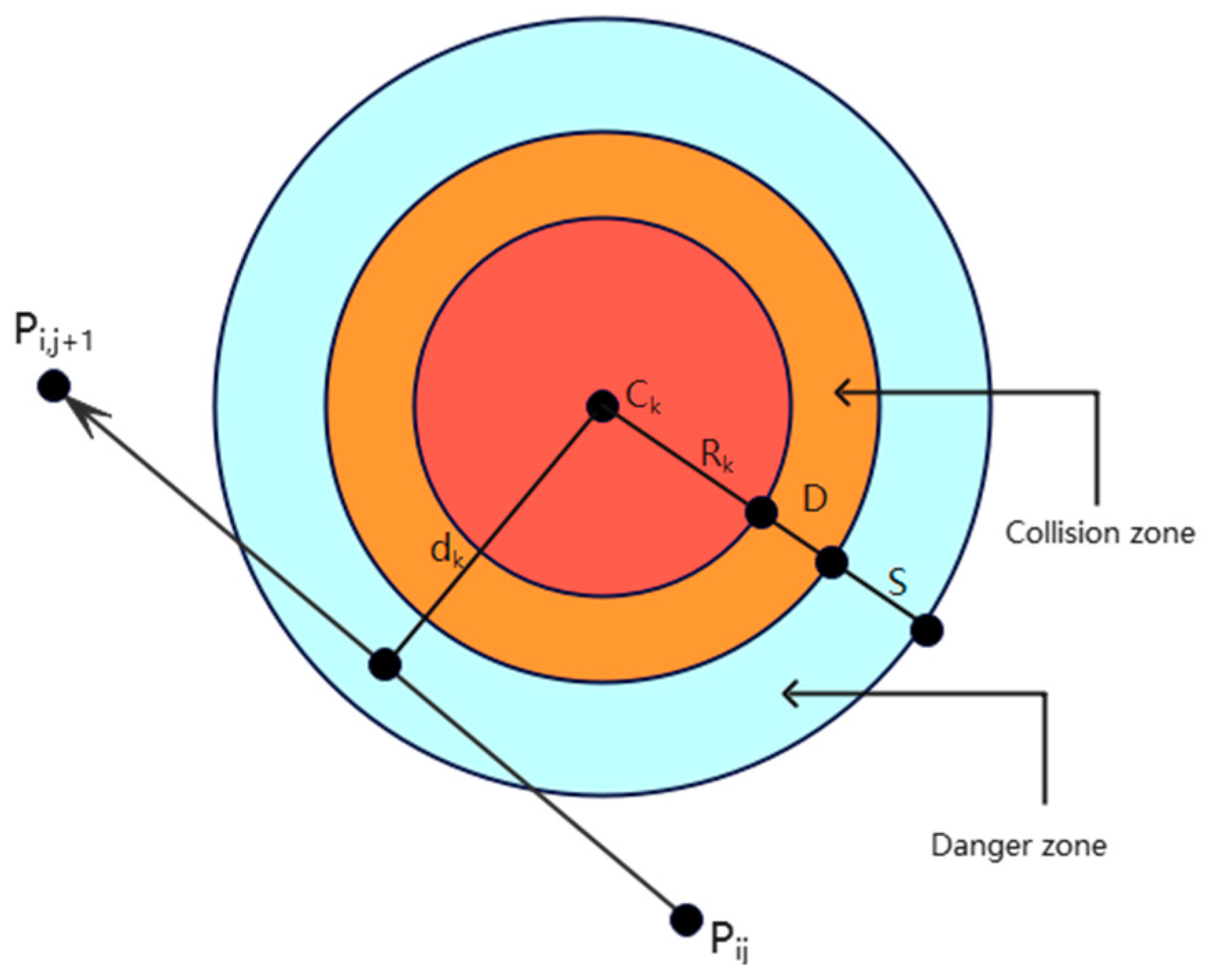
2.2. Security Cost Function

Besides the optimal flight distance, the optimal path also needs to focus on flight safety factors. In the experiment of this paper, we assume that each obstacle in the path is represented by a cylinder and suppose that $K$ is the set of all threatening obstacles, $C_k$ is the coordinate of the center of the obstacle and the radius of the obstacle is $R_k$. Figure 1 shows the obstacle threat figure from the path node $P_{ij}$ to the path node $P_{i,j+1}$. $D$ is the diameter of the UAV, $S$ represents the danger distance between the UAV and the collision domain and $d_k$ represents the distance between the UAV path and the center of the obstacle $C_k$. There are several factors that affect the danger distance $S$, such as operating environment, signal strength and positioning accuracy. For example, the value of $S$ can be taken smaller when the GPS signal is strong and vice versa when $S$ is taken larger. In summary, for the obstacle set $K$, the security cost function $F_2$ for $P_{ij}$ to $P_{i,j+1}$ can be summarized by Equations (2) and (3).

$$F_2(X_i)={\displaystyle \sum _{j=1}^{n-1}{\displaystyle \sum _{k=1}^K{T}_k}(\overrightarrow{P_{ij}{P}_{i,j+1}})}$$

(2)

$$T_k(\overrightarrow{P_{ij}{P}_{i,j+1}})=\left\{\begin{array}{ll}0,& \mathrm{if} d_k>S+D+R_k\\ (S+D+R_k)-d_k,& \mathrm{if} D+R_k<d_k\le S+D+R_k\\ \infty ,& \mathrm{if} d_k\le D+R_k\end{array}\right.$$

(3)

2.3. Flight Altitude Cost Function

When a UAV executes its mission, its flight altitude is usually limited to a certain range. For example, when using a UAV for aerial photography, the clarity of the aerial photos has some relationship with the flight altitude. The flight altitude cost function of the UAV can be described by Equations (4) and (5).

$$F_3(X_i)={\displaystyle \sum _{j=1}^n{H}_{ij}}$$

(4)

$$H_{ij}=\left\{\begin{array}{ll}\mid h_{ij}-\frac{(h_{\max }+h_{\min })}{2}\mid ,& \mathrm{if} h_{\min }\le h_{ij}\le h_{\max }\\ \infty , \mathrm{otherwise}\end{array}\right.$$

(5)

where $h_{ij}$ is the flight altitude of the UAV relative to the ground and $h_{\max }$ and $h_{\min }$ are the maximum and minimum values of the flight altitude scope. The flight altitude scope of UAV is shown in Figure 2.

2.4. Smooth Cost

Smoothing cost is used to calculate the rotation angle and climb speed required for the UAV during flight. Figure 3 shows the 3D coordinate schematic of the UAV flight from $P_{ij}$ to $P_{i,j+2}$. $P_{ij}{}^{\prime }$, $P_{i,j+1}^{\prime }$ and $P_{i,j+2}^{\prime }$ are the projections of coordinate points $P_{ij}$, $P_{i,j+1}$ and $P_{i,j+2}$ on the XOY plane. We project the three-dimensional flight path of the UAV onto the XOY plane of the coordinate axis, and the angle formed by the extension of the path $P_{ij}{}^{\prime }$ to $P_{i,j+1}^{\prime }$ and the path $P_{i,j+1}^{\prime }$ to $P_{i,j+2}^{\prime }$ is noted as ${\varphi }_{ij}$. The vector $\overrightarrow{P_{ij}{}^{\prime }{P}_{i,j+1}^{\prime }}$ can be calculated using Equation (6).

$$\overrightarrow{P_{ij}{}^{\prime }{P}_{i,j+1}^{\prime }}=\overrightarrow{k}\times (\overrightarrow{P_{ij}{P}_{i,j+1}}\times \overrightarrow{k})$$

(6)

where $\overrightarrow{k}$ is the unit vector in the z-axis direction. ${\varphi }_{ij}$ is calculated as follows:

$${\varphi }_{ij}=\arctan \left(\frac{‖\overrightarrow{{P_{ij}}^{\prime }{P_{i,j+1}}^{\prime }}\times \overrightarrow{{P_{i,j+1}}^{\prime }{P_{i,j+2}}^{\prime }}‖}{\overrightarrow{{P_{ij}}^{\prime }{P_{i,j+1}}^{\prime }}\cdot \overrightarrow{{P_{i,j+1}}^{\prime }{P_{i,j+2}}^{\prime }}}\right)$$

(7)

$P_{i,j+2}^{\prime \prime }$ is the projection point of the projection of $P_{i,j+2}$ onto the plane where the vector $\overrightarrow{P_{ij}{P}_{i,j+1}}$ is located. The angle formed by the vector $\overrightarrow{P_{i,j+1}{P}_{i,j+2}}$ and the vector $\overrightarrow{P_{i,j+1}{P}_{i,j+2}^{\prime \prime }}$ is denoted as ${\theta }_{i,j+1}$ and is calculated as follows:

$${\theta }_{ij+1}=\arctan \left(\frac{z_{i,j+1}-z_{ij}}{‖\overrightarrow{P_{ij}{}^{\prime }{P}_{i,j+1}{}^{\prime }}‖}\right)$$

(8)

In summary, the equation for the smooth cost $F_4$ is as follows:

$$F_4=a_1{\displaystyle \sum _{j=1}^{n-2}{\varphi }_{ij}+a_2}{\displaystyle \sum _{j=1}^{n-1}\left|{\theta }_{ij}-{\theta }_{i,j-1}\right|}$$

(9)

where $a_1$ is the penalty factor for the turn angle in the UAV flight path and $a_2$ is the penalty factor for the climb angle in the UAV flight path.

2.5. Integrated Cost Function for UAV Path Planning

When choosing the optimal path, the UAV has to consider the distance cost, flight altitude cost, safety cost and smoothing cost to finally plan an optimal path that is safe and efficient. Combining $F_1$~$F_4$ the mathematical model of the final cost function of UAV path planning is as follows:

$$F(X_i)={\displaystyle \sum _{k=1}^4{b}_k{F}_k(X_i)}$$

(10)

where $b_k$ represents the weight coefficient of the $k$th cost function. The set $X_i$ includes the coordinates of the n path nodes $P_{ij}=(x_{ij},y_{ij},z_{ij})$. The cost function $F(X_i)$ perfectly establishes an NP-hard mathematical model for the optimization objectives and constraints of the UAV path planning problem, which provides sufficient conditions for the subsequent experiments of this paper to use metaheuristic algorithms to optimize the UAV path planning problem.

2.6. Spherical Vector-Based UAV Path Planning Method

The spherical vector-based UAV path planning method encodes each feasible path from the start point to the end point as a set of vectors. In this method, each vector specifically describes the flight motion of the UAV during flight from one path node to the next path node. Each vector in the vector group of the UAV path planning method based on spherical vectors is composed of three vectors: $\rho \in (0,path\_length)$, $\theta \in (-\pi /2,\pi /2)$ and $\varphi \in (-\pi ,\pi )$. $\rho$ represents the magnitude, $\theta$ represents the flight elevation angle of the UAV and $\varphi$ represents the flight azimuth of the UAV. Thus, each feasible path ${\Omega }_i$ with $n$ flight nodes can be represented by a set of 3N-dimensional spherical vectors as follows:

$${\Omega }_i=({\rho }_{i1},{\theta }_{i1},{\varphi }_{i1},{\rho }_{i2},{\theta }_{i2},{\varphi }_{i2},\cdots ,{\rho }_{in},{\theta }_{in},{\varphi }_{in})$$

(11)

The basic principle of the spherical vector-based path planning method is to utilize the relationship between the magnitude, elevation and azimuth angles during flight and the speed, turn angle and climb angle of the UAV to improve the safety and effectiveness of the planned path. The spherical vector-based method can help the metaheuristic algorithm search in configuration space instead of Cartesian space; therefore, it can effectively minimize the search space of the algorithm and thus increase the algorithm’s ability to discover a better flight path for the UAV.

3. Basic Tuna Swarm Optimization Algorithm

The tuna swarm optimization algorithm is a novel metaheuristic algorithm created by modeling the spiral feeding behavior and parabolic feeding behavior of tuna swarm. TSO has been widely studied and applied once it was proposed. Wumaier Tuerxun et al. improved TSO using the tent chaotic mapping strategy and the parameter adjustment strategy and applied the algorithm to improve the accuracy of wind speed prediction for wind farms [35]. Wang et al. improved TSO using the circle chaotic mapping strategy, Lévy operator and nonlinear adaptive operator to enhance the comprehensive optimization performance of TSO and used the modified algorithm to improve the classification performance of the BP neural network [36]. Jingyu Wang et al. used the chaos factor to modify the TSO algorithm and proved that the modified algorithm has excellent effects on forest canopy image segmentation [37].

3.1. TSO Initialization

Assuming there are N individuals in the tuna population, the TSO can be initialized using Equation (12).

$$\begin{array}{c}{X}_i^{}=rand\cdot (ub-lb)+lb=\left[\begin{array}{cccc}{x}_i^1& x_i^2& \cdots & x_i^j\end{array}\right]\\ \left\{\begin{array}{c}i=1,2,\dots ,N\\ j=1,2,\dots ,Dim\end{array}\right.\end{array}$$

(12)

where $X_i^{}$ is the $i$th candidate solution which is also the $i$th tuna in the TSO algorithm; $lb$ and $ub$ are the lower and upper bounds of the solution space. Each candidate solution in TSO has $Dim$ dimensions.

3.2. The Parabolic Feeding Strategy of the TSO

Tuna usually chose eel and squid, etc., as the main catching target. Since these preys are very agile, it is difficult for a single tuna to catch the prey independently. Therefore, the elite of tuna will organize a swarm of fish together to attack the prey cooperatively. In the cooperative attack behavior, the tuna will follow the companion in front of them to form a parabolic shape of the whole population to close in on the prey; biologists called this behavior the tuna parabolic foraging strategy. This swarm behavior can be modeled using Equations (13) and (14).

$$X_i^{t+1}=\left\{\begin{array}{cc}{X}_{best}^t+rand\cdot (X_{best}^t-X_i^t)+TF\cdot p^2\cdot (X_{best}^t-X_i^t),& \mathrm{if} \mathrm{rand} <0.5\\ TF\cdot p^2\cdot X_i^t,\hfill & \mathrm{if} \mathrm{rand}\ge 0.5\end{array}\right.$$

(13)

$$p={(1-\frac{t}{t_{\max }})}^{(t/t_{\max })}$$

(14)

where $X_{best}^t$ is the optimal individual during the $i$th algorithm execution, $X_i^t$ is the tuna individual during the $t$th algorithm execution and $X_{i+1}^t$ is the new individual generated during the $t+1$th execution. The value of $TF$ is a randomly selected value of 1 or −1.

3.3. The Spiral Foraging Strategy of the TSO

In the long-term hunting action, the tuna swarm also gradually formed another kind of population hunting strategy; biologists call this strategy spiral hunting strategy. When the tuna group executes this strategy, the whole population will swarm together to form a spiral vortex; at this time, the swimming of the tuna group will not only be influenced by the best individual, but they will also occasionally follow the other part of the swarm to search. Inspired by the spiral foraging of tuna, scholars proposed the spiral renewal strategy of TSO. In the spiral foraging strategy of TSO, the position update of tuna in the population will be pulled by the optimal individuals; in addition, the position update of tuna will occasionally be influenced by random individuals in the population, and the spiral foraging approach of TSO can be modeled using Equations (15)–(19). In TSO, the two foraging methods are randomly selected.

$$X_i^{t+1}=\left\{\begin{array}{c}{\alpha }_1\cdot \left(X_{\mathit{rand} }^t+\tau \cdot \left|X_{\mathit{rand} }^t-X_i^t\right|\right)+{\alpha }_2\cdot X_i^t,\\ i=1\\ {\alpha }_1\cdot \left(X_{\mathit{rand} }^t+\tau \cdot \left|X_{\mathit{rand} }^t-X_i^t\right|\right)+{\alpha }_2\cdot X_{i-1}^t,\\ \hspace{1em}\hspace{1em}\hspace{1em}i=2,3,\dots ,N\\ {\alpha }_1\cdot \left(X_{\mathit{best} }^t+\tau \cdot \left|X_{\mathit{best} }^t-X_i^t\right|\right)+{\alpha }_2\cdot X_i^t,\\ i=1,\\ {\alpha }_1\cdot \left(X_{\mathit{best} }^t+\tau \cdot \left|X_{\mathit{best} }^t-X_i^t\right|\right)+{\alpha }_2\cdot X_{i-1}^t,\\ \hspace{1em}\hspace{1em}\hspace{1em}i=2,3,\dots ,N\end{array}\begin{array}{c}, \mathit{if} \mathrm{rand} <\frac{t}{t_{max}}\\ \\ \\ , \mathit{if} \mathrm{rand} \ge \frac{t}{t_{max}}\end{array}\right.$$

(15)

$${\alpha }_1=a+(1-a)\cdot \frac{t}{t_{\max }}$$

(16)

$${\alpha }_2=(1-a)-(1-a)\cdot \frac{t}{t_{\max }}$$

(17)

$$\tau =e^{bl}\cdot \cos (2\pi b)$$

(18)

$$l=e^{3\cos (((t_{\max }+1/t)-1)\pi )}$$

(19)

$X_{rand}^t$ is the position of one other tuna randomly selected in the population as a reference during the position update of the tuna, ${\alpha }_1$ is the weight coefficient that controls the closeness of individual tuna swimming toward the optimal tuna or random tuna and ${\alpha }_2$ is the weight coefficient that controls the swimming of tuna toward the previous tuna. $a$ is a constant, and in this paper, $a$ = 0.7. $t$ and $t_{\max }$ represent the current and maximum number of iterations.

3.4. Pseudo-Code of TSO

The pseudo-code for TSO is as shown in Algorithm 1.

Algorithm 1 Pseudo-code of TSO Algorithm

Initialization: Set parameters N, Dim, a, z and $t_{\max }$ Initialize the position of tuna Xi (i = 1, 2, …, N) by (1),Counter t = 0 while t < $t_{\max }$ do  Calculate the fitness value of all tuna  Update the position and value of the best tuna $X_{best}^t$  for (each tuna) do    Update ${\alpha }_1$, ${\alpha }_2$ and $p$ by (16), (17), (14)     if (rand < z) then      Update $X_i^{t+1}$ by (12)     else if ($rand\ge z$) then       if (rand < 0.5) then        Update $X_i^{t+1}$ by (15)       else if ($rand\ge 0.5$) then        Update $X_i^{t+1}$ by (13)       end if     end if   end for  end while  t = t + 1  return the best fitness value f ($X_{best}^{}$) and the best tuna $X_{best}^{}$

4. The Proposed SGGTSO

To enhance the comprehensive optimization performance of the TSO algorithm as well as the applicability of the TSO algorithm to the 3-dimensional UAV path planning problem, this paper proposes a multi-group sigmoid nonlinear parameter Gaussian mutation elite individual genetic strategy tuna swarm optimization algorithm (SGGTSO).

4.1. Sigmoid Nonlinear Weighting Operators

In the TSO algorithm, the parameter $p$ in Equation (14) is a key factor in controlling and balancing the global exploitation and local exploration capabilities of TSO. A quality metaheuristic algorithm needs to strictly control the global and local search ability. During the research of metaheuristics, many scholars proved that optimizing the weight coefficients of the algorithm or introducing nonlinear parameters into the algorithm can significantly optimize the comprehensive performance of the algorithm [38,39,40,41]. In the initial search phase of the metaheuristic algorithm, there is a huge gap between almost all candidate solutions in the algorithm and the global optimal solution; therefore, the global exploitation ability needs to be enhanced in the initial search phase of the metaheuristic algorithm. In the later stage of the search of the metaheuristic algorithm, the gap between the candidate solutions found in the algorithm and the optimal solution is smaller; so at this time, the local exploration ability of the algorithm needs to be improved to fine-tune the candidate solution set so as to improve the probability of the algorithm to find the optimal solution.

Sigmoid is a very classical activation function in deep learning theory, and its mathematical model can be represented by Equation (20).

$$S(x)=\frac{1}{1+e^{-x}},x\in R$$

(20)

The derivative curve of sigmoid is centered at the origin $O$ and decreases to the positive and negative directions of the X-axis, respectively, and its derivative values at $(-\infty ,-5)$ and $(5,+\infty )$ tend to 0. In this paper, the $[-5,5]$ part of the sigmoid derivative curve is applied to modify the weight coefficient $p$. The equation of the improved $p_1$ can be expressed by Equation (21).

$$p_1=\frac{1}{1+1.5e^{\frac{10t}{t_{\max }}-5}}-0.1r$$

(21)

where $t$ and $t_{\max }$ are the current iteration and the maximum iteration, respectively. $r$ is a random value between $(0,1)$.

Analysis for Equations (13) and (14) reveals that the global and local optimization ability of TSO is closely related to the $p^2$. Figure 4 shows the comparison curves of the modified weighting coefficient $p_1^2$ and the weighting coefficient $p^2$ in the original TSO. Compared to the original weight parameter $p^2$, the modified weight parameter $p_1^2$ using sigmoid has significant volatility. The irregular fluctuation helped the tuna individuals to update to get more uniform positions when executing the parabolic foraging strategy, thus further enriching the population diversity of the algorithm. The weight factor $p_1^2$ decreases rapidly during the iterative process, which can help the algorithm to move from global development to local exploration relatively smoothly.

4.2. Multi-Subgroup Gaussian Mutation Strategy

Taking the metaheuristic algorithm to deal with the minimization optimization problem as an example, in this paper, while keeping the original population size of TSO unchanged, the population individuals are sorted according to the fitness value from smallest to largest; the sub-swarm with the smaller fitness value is called the elite swarm, and the other swarm is called the ordinary swarm, and these two types of swarms perform different Gaussian mutation strategies, respectively.

4.2.1. Gaussian Mutation Strategy Based on Elite Learning Mechanism

Using the elite learning strategy for the tuna individuals in the elite swarm, the elite learning mechanism enhances the ability of elite tuna individuals to escape from local extremes, thus achieving that the elite tuna guide the other tuna individuals to update their positions, and thus accelerating the convergence of the algorithm.

The equation of Gaussian distribution is as follows:

$$Gauss(t)=\frac{1}{\sigma \sqrt{2\pi }}\exp (-\frac{{(t-u)}^2}{2{\sigma }^2})$$

(22)

where $u=0$. The variance $\sigma$, which is the learning rate, is calculated as shown in Equation (23).

$$\sigma ={\sigma }_{\max }-({\sigma }_{\max }-{\sigma }_{\min })\frac{t}{t_{\max }}$$

(23)

where ${\sigma }_{\max }=1$ and ${\sigma }_{\min }=0.1$. The learning rate $\sigma$ decreases as the number of iterations increases, which can help the Gaussian distribution function to obtain a wider search range at the beginning of the iteration, thus helping the elite tuna individuals to jump out of the local optimum more easily. Conversely, in the later iteration, the Gaussian distribution is concentrated in a smaller area, thus helping the tuna individuals to explore finely in the area near the origin, which is helpful to improve the convergence accuracy of SGGTSO.

In summary, the mathematical modeling of Gaussian variation strategies based on elite learning for an elite swarm is as follows:

$$X_i^{t+1}=X_i^t+r\cdot \frac{1}{2}{t}^2\frac{X_{best}^t-X_{worst}^t}{2}Gauss(t)$$

(24)

$$r=\left\{\begin{array}{l}1,if rand\ge 0.5\\ 0,otherwise\end{array}\right.$$

(25)

where the value of $rand$ is a random number within $(0,1)$.

4.2.2. Non-Uniform Gaussian Mutation Strategy

Individuals at the tail end of the tuna group have worse fitness values, so this subgroup is called the ordinary population. Tuna individuals in this type of ordinary swarm can better retain their own characteristics instead of only following elite individuals to update their positions. In order to further increase the population diversity of tuna swarms, this paper uses a non-uniform Gaussian mutation strategy [42] for tuna in ordinary populations, and the details are as follows:

$$X_i^{t+1}=X_i^t+\Delta (t,G_i^t)$$

(26)

$$\Delta (t,y)=y(1-r^{{(\frac{1-t}{t_{\max }})}^2})$$

(27)

$$G_i^t=N((X_{best}^t-X_i^t),\sigma )$$

(28)

where $\Delta (t,G_i^t)$ is the non-uniform Gaussian mutation step, which is the mutation operator obtained by adaptively adjusting the step size through the Gaussian distribution ($G_i^t$). $r$ is a random number uniformly generated in the interval $[0,1]$, $\sigma$ is the standard deviation of the Gaussian distribution and the expectation value of the Gaussian distribution is $(X_{best}^t-X_i^t)$. In the experiments in this paper, $\sigma$= 1.

The non-uniform Gaussian mutation strategy selects the difference between the optimal individual and the current tuna individual as the expectation value and uses an adaptive adjustment learning strategy for the step size of Gaussian mutation, this update method helps to maintain the diversity of the population, thus better balancing the global exploitation and local exploration of SGGTSO.

4.3. Elite Individual Genetic Strategy

Genetic algorithm (GA) [43] is a classical metaheuristic algorithm that mimics the evolutionary genetic cross-genetic inheritance of organisms in nature. In this paper, the basic methods of TSO and GA are merged so that the SGGTSO algorithm proposed in this paper can combine the advantages of both algorithms [44]. The three tuna individuals with the best fitness values in the population were selected as the main genetic targets.

During the SGGTSO iteration, the three selected tuna ($g{i}_1$~$g{i}_3$) individuals with the best fitness value are compared with all individuals ($g{j}_1$~$g{j}_N$), and if tuna $i$ has a better fitness value than tuna $j$, then tuna $i$ is genetically crossed with tuna $j$. On the contrary, tuna $i$ and tuna $j$ are genetically mutated.

Each genetic crossover process will produce two new individuals, $New{X}_j^i$ and $New{X}_j^{i+1}$. The equation for tuna genetic crossover is as follows:

$$New{X}_j^i=(r+1)\cdot X_j^{gi}+(1-r)\cdot X_j^{gj},i\in [1,N],j\in [1,Dim]$$

(29)

$$New{X}_j^{i+1}=(r+1)\cdot X_j^{gj}+(1-r)\cdot X_j^{gi},i\in [1,N],j\in [1,Dim]$$

(30)

where $X_j^i$, $X_j^{\mathrm{g}i}$ and $X_j^{\mathrm{gj}}$ denote gene $j$ of the $X^i$, $X^{gi}$ and $X^{gj}$, respectively. $r$ is a random number in the range $[0,2]$.

Each genetic mutation process will also produce two new tuna individuals, $New{X}_j^i$ and $New{X}_j^{i+1}$. In the gene mutation process, the probability of gene mutation is set to $\mu$, which means that $\mu \ast \mathrm{Dim}$ genes will mutate in individual tuna $New{X}_j^i$ and $New{X}_j^{i+1}$. The equation for tuna genetic mutation is as follows:

$$New{X}_j^i=X_j^{gi}+\delta \cdot \gamma ,i\in [1,N],j\in [1,\mu \ast \mathrm{Dim}]$$

(31)

$$New{X}_j^{i+1}=X_j^{gj}+\delta \cdot \gamma ,i\in [1,N],j\in [1,\mu \ast \mathrm{Dim}]$$

(32)

$$\delta =0.1\cdot (ub-lb)$$

(33)

where $ub$ and $lb$ are the boundaries of the SGGTSO search space. $\gamma$ is a random value that conforms to a normal distribution.

After the crossover and mutation process of the tuna population, a new swarm $NewX$ can be created, and then $NewX$ can be fused with the original tuna population $X$. Finally, the individuals with excellent fitness values are retained according to the elite selection strategy, while maintaining no change in the population size. The elite individual genetic strategy greatly enriches the swarm diversity of the tuna population by crossover and mutation operations on individuals in the swarm. In addition, the worse individuals in the population can acquire the genes of the superior individuals in the swarm, thus ensuring that the tuna individuals in the swarm are always maintained at a high-quality level. Therefore, the elite individual genetic strategy can significantly accelerate the convergence rate of SGGTSO.

4.4. Pseudo-Code of SGGTSO

The pseudo-code for SGGTSO is shown in Algorithm 2.

Algorithm 2 Pseudo-code of SGGTSO Algorithm

Initialization: Set parameters N, Dim, a, z and $t_{\max }$ Initialize the position of tuna Xi (i = 1, 2, …, N) by (1) Counter t = 0 while t < $t_{\max }$ do  Calculate the fitness value of all tuna  Update the position and value of the best tuna $X_{best}^t$  for (i=1:N/2) do     Update ${\alpha }_1$, ${\alpha }_2$ and $p_1^2$ by (16), (17), (21)       if (rand < z) then      Update $X_i^{t+1}$ by (12)       else if ($rand\ge z$) then       if (rand < 0.5) then          Update $X_i^{t+1}$ by (15) and subsequently by (24)       else if ($rand\ge 0.5$) then          Update Update $X_i^{t+1}$ by (13) subsequently by (24)       end if     end if  end for  for (i=N/2+1:N) do     Update ${\alpha }_1$, ${\alpha }_2$ and $p$ by (16), (17), (21)      if (rand < z) then        Update $X_i^{t+1}$ by (12)      else if ($rand\ge z$) then        if (rand < 0.5) then         Update $X_i^{t+1}$ by (15) and subsequently by (26)        else if ($rand\ge 0.5$) then         Update $X_i^{t+1}$ by (13) subsequently by (26)        end if       end if   end for     Update $X$ by Elite individual genetic strategy     t = t + 1  end while  return the best fitness value f ($X_{best}^{}$) and the best tuna $X_{best}^{}$

5. Comparative Experiments and Data Analysis

In order to evaluate whether the SGGTSO proposed in this paper has significant advantages over some other classical and novel metaheuristics, the CEC2017, a classical and authoritative collection of benchmark functions, is selected for a comprehensive test of SGGTSO.

5.1. Details of the Benchmark Function Set

The CEC2017 benchmark function [45] collection is a highly authoritative collection of functions for testing the comprehensive outperformance of metaheuristics, which covers unimodal, multimodal, hybrid and conforming functions. In this paper, CEC2017 is applied to evaluate SGGTSO comprehensively and extensively, and the details of the CEC2017 test function set are shown in

Table 1. CEC2017 benchmark functions.

Function	Function Number	Dim	Range	${\mathbf{f}}_{\mathbf{min}}$
Shifted and Rotated Bent Cigar Function	F1	100	[−100, 100]	100
Shifted and Rotated Zakharov Function	F2	100	[−100, 100]	300
Shifted and Rotated Rosenbrock’s Function	F3	100	[−100, 100]	400
Shifted and Rotated Rastrigin’s Function	F4	100	[−100, 100]	500
Shifted and Rotated Expanded Scaffer’s F6 Function	F5	100	[−100, 100]	600
Shifted and Rotated Lunacek Bi_Rastrigin Function	F6	100	[−100, 100]	700
Shifted and Rotated Non-Continuous Rastrigin’s Function	F7	100	[−100, 100]	800
Shifted and Rotated Levy Function	F8	100	[−100, 100]	900
Shifted and Rotated Schwefel’s Function	F9	100	[−100, 100]	1000
Hybrid Function 1 (N = 3)	F10	100	[−100, 100]	1100
Hybrid Function 2 (N = 3)	F11	100	[−100, 100]	1200
Hybrid Function 3 (N = 3)	F12	100	[−100, 100]	1300
Hybrid Function 4 (N = 4)	F13	100	[−100, 100]	1400
Hybrid Function 5 (N = 4)	F14	100	[−100, 100]	1500
Hybrid Function 6 (N = 4)	F15	100	[−100, 100]	1600
Hybrid Function 6 (N = 5)	F16	100	[−100, 100]	1700
Hybrid Function 6 (N = 5)	F17	100	[−100, 100]	1800
Hybrid Function 6 (N = 5)	F18	100	[−100, 100]	1900
Hybrid Function 6 (N = 6)	F19	100	[−100, 100]	2000
Composition Function 1 (N = 3)	F20	100	[−100, 100]	2100
Composition Function 2 (N = 3)	F21	100	[−100, 100]	2200
Composition Function 3 (N = 4)	F22	100	[−100, 100]	2300
Composition Function 4 (N = 4)	F23	100	[−100, 100]	2400
Composition Function 5 (N = 5)	F24	100	[−100, 100]	2500
Composition Function 6 (N = 5)	F25	100	[−100, 100]	2600
Composition Function 7 (N = 6)	F26	100	[−100, 100]	2700
Composition Function 8 (N = 6)	F27	100	[−100, 100]	2800
Composition Function 9 (N = 3)	F28	100	[−100, 100]	2900
Composition Function 10 (N = 3)	F29	100	[−100, 100]	3000

. $F_1$~$F_2$ are unimodal functions, $F_3$~$F_9$ are unimodal functions, $F_{10}$~$F_{19}$ are hybrid functions and $F_{20}$~$F_{29}$ are composition functions.

5.2. Competition Algorithms and Experimental Parameter Settings

The comparison experiments in this paper are chosen for the case of the CEC2017 benchmark function with dimension 100, and the algorithms Accelerated Particle Swarm Optimization (APSO) [46], Artificial Rabbits Optimization (ARO) [47], Beluga Whale Optimization (BWO), Whale Optimization Algorithm (WOA) [48] and TSO are chosen as control group experiments to compare with SGGTSO. It is worth mentioning that APSO is an improved version of the classical algorithm PSO, and ARO and BWO are novel metaheuristics that have been proposed recently.

In the experiments of this paper, the maximum number of iterations is set to 1000, and the population size of each algorithm is set to 30. In order to make the experimental results more convincing, the experiments are repeated 15 times and the data, such as the mean value of each algorithm, are published in this paper. The parameter settings for each algorithm are detailed in

Table 2. Parameter setting for each algorithm.

Algorithm	Parameter Value
APSO	$\alpha =1,\beta =0.5$
ARO	$~$
BWO	$W_f\in \left[0.05,0.1\right]$
WOA	$b=1$
TSO	$\begin{array}{l}a=0.7, z=0.05\hfill \end{array}$
SGGTSO	$\begin{array}{l}a=0.7, z=0.05\hfill \end{array},\mu =0.05$

. The symbol $~$ means that the algorithm has no preset parameters.

5.3. Experimental Results and Numerical Analysis

Table 3. Experimental results of each algorithm in CEC2017.

Function	Performance	APSO	ARO	BWO	WOA	TSO	SGGTSO
$F_1$	Mean	2.86 × 10+11	8.70 × 10+09	2.54 × 10+11	6.36 × 10+10	3.54 × 10+09	2.18 × 10+05
	Std	2.78 × 10+10	2.39 × 10+09	7.02 × 10+09	5.66 × 10+09	1.27 × 10+09	8.23 × 10+04
$F_2$	Mean	6.29 × 10+05	3.40 × 10+05	3.51 × 10+05	8.97 × 10+05	3.86 × 10+05	1.33 × 10+05
	Std	1.31 × 10+05	1.91 × 10+04	1.40 × 10+04	1.78 × 10+05	6.45 × 10+04	1.94 × 10+04
$F_3$	Mean	8.66 × 10+04	2.22 × 10+03	9.46 × 10+04	1.24 × 10+04	1.48 × 10+03	7.72 × 10+02
	Std	1.53 × 10+04	2.99 × 10+02	6.56 × 10+03	2.27 × 10+03	1.81 × 10+02	6.07 × 10+01
$F_4$	Mean	1.86 × 10+03	1.29 × 10+03	2.11 × 10+03	1.90 × 10+03	1.33 × 10+03	1.26 × 10+03
	Std	1.31 × 10+02	6.92 × 10+01	3.24 × 10+01	1.63 × 10+02	6.04 × 10+01	6.74 × 10+01
$F_5$	Mean	6.82 × 10+02	6.45 × 10+02	7.12 × 10+02	7.03 × 10+02	6.67 × 10+02	6.38 × 10+02
	Std	6.48	5.98	1.80	7.60	4.19	8.03
$F_6$	Mean	5.44 × 10+03	2.70 × 10+03	3.85 × 10+03	3.64 × 10+03	3.05 × 10+03	2.51 × 10+03
	Std	2.47 × 10+02	2.63 × 10+02	7.15 × 10+01	1.96 × 10+02	1.90 × 10+02	2.50 × 10+02
$F_7$	Mean	2.28 × 10+03	1.63 × 10+03	2.58 × 10+03	2.33 × 10+03	1.77 × 10+03	1.66 × 10+03
	Std	1.00 × 10+02	9.38 × 10+01	3.17 × 10+01	1.25 × 10+02	1.00 × 10+02	8.88 × 10+01
$F_8$	Mean	3.79 × 10+04	2.87 × 10+04	7.87 × 10+04	7.12 × 10+04	2.91 × 10+04	2.28 × 10+04
	Std	4.54 × 10+03	3.24 × 10+03	3.22 × 10+03	1.78 × 10+04	6.21 × 10+03	2.18 × 10+03
$F_9$	Mean	2.44 × 10+04	1.72 × 10+04	3.23 × 10+04	2.78 × 10+04	2.11 × 10+04	1.60 × 10+04
	Std	1.17 × 10+03	1.34 × 10+03	5.04 × 10+02	1.67 × 10+03	3.41 × 10+03	1.78 × 10+03
$F_{10}$	Mean	3.90 × 10+05	4.67 × 10+04	2.75 × 10+05	2.36 × 10+05	4.36 × 10+04	2.27 × 10+03
	Std	1.10 × 10+05	1.46 × 10+04	4.67 × 10+04	1.16 × 10+05	1.34 × 10+04	2.17 × 10+02
$F_{11}$	Mean	1.78 × 10+11	5.95 × 10+08	1.88 × 10+11	1.28 × 10+10	3.13 × 10+08	4.11 × 10+07
	Std	3.52 × 10+10	1.19 × 10+08	9.99 × 10+09	3.44 × 10+09	1.70 × 10+08	1.41 × 10+07
$F_{12}$	Mean	4.23 × 10+10	1.18 × 10+05	4.31 × 10+10	5.64 × 10+08	9.76 × 10+04	8.65 × 10+03
	Std	6.95 × 10+09	4.64 × 10+04	2.26 × 10+09	2.23 × 10+08	5.46 × 10+04	4.82 × 10+03
$F_{13}$	Mean	7.12 × 10+07	3.17 × 10+06	8.15 × 10+07	1.41 × 10+07	9.99 × 10+05	8.47 × 10+05
	Std	5.12 × 10+07	1.66 × 10+06	2.44 × 10+07	6.51 × 10+06	5.23 × 10+05	3.51 × 10+05
$F_{14}$	Mean	1.79 × 10+10	1.34 × 10+04	2.18 × 10+10	1.04 × 10+08	2.07 × 10+04	3.95 × 10+03
	Std	3.14 × 10+09	1.58 × 10+04	2.46 × 10+09	7.41 × 10+07	8.60 × 10+03	1.77 × 10+03
$F_{15}$	Mean	1.71 × 10+04	6.01 × 10+03	2.23 × 10+04	1.56 × 10+04	6.46 × 10+03	6.07 × 10+03
	Std	2.83 × 10+03	5.72 × 10+02	1.55 × 10+03	2.22 × 10+03	7.89 × 10+02	5.85 × 10+02
$F_{16}$	Mean	3.51 × 10+06	5.01 × 10+03	3.68 × 10+06	1.29 × 10+04	6.40 × 10+03	5.91 × 10+03
	Std	3.56 × 10+06	5.52 × 10+02	1.90 × 10+06	4.27 × 10+03	7.86 × 10+02	4.75 × 10+02
$F_{17}$	Mean	1.10 × 10+08	3.52 × 10+06	1.59 × 10+08	1.21 × 10+07	1.40 × 10+06	1.16 × 10+06
	Std	7.05 × 10+07	1.65 × 10+06	5.53 × 10+07	6.90 × 10+06	7.71 × 10+05	3.89 × 10+05
$F_{18}$	Mean	1.64 × 10+10	9.82 × 10+03	2.10 × 10+10	1.40 × 10+08	4.89 × 10+04	5.14 × 10+03
	Std	2.92 × 10+09	4.26 × 10+03	3.07 × 10+09	1.22 × 10+08	4.92 × 10+04	4.28 × 10+03
$F_{19}$	Mean	6.16 × 10+03	5.23 × 10+03	7.61 × 10+03	6.60 × 10+03	5.68 × 10+03	5.04 × 10+03
	Std	5.31 × 10+02	3.80 × 10+02	3.31 × 10+02	5.62 × 10+02	7.06 × 10+02	4.18 × 10+02
$F_{20}$	Mean	4.91 × 10+03	3.09 × 10+03	4.71 × 10+03	4.36 × 10+03	3.36 × 10+03	3.18 × 10+03
	Std	2.26 × 10+02	6.34 × 10+01	8.29 × 10+01	2.06 × 10+02	1.18 × 10+02	8.59 × 10+01
$F_{21}$	Mean	2.78 × 10+04	2.01 × 10+04	3.43 × 10+04	3.04 × 10+04	2.35 × 10+04	1.93 × 10+04
	Std	9.26 × 10+02	1.54 × 10+03	9.49 × 10+02	1.56 × 10+03	3.25 × 10+03	2.09 × 10+03
$F_{22}$	Mean	7.41 × 10+03	3.61 × 10+03	6.08 × 10+03	5.14 × 10+03	4.70 × 10+03	3.85 × 10+03
	Std	6.58 × 10+02	1.07 × 10+02	1.32 × 10+02	2.67 × 10+02	3.84 × 10+02	2.28 × 10+02
$F_{23}$	Mean	1.35 × 10+04	4.69 × 10+03	9.12 × 10+03	6.62 × 10+03	6.39 × 10+03	4.89 × 10+03
	Std	9.35 × 10+02	1.68 × 10+02	4.36 × 10+02	3.63 × 10+02	7.44 × 10+02	1.48 × 10+02
$F_{24}$	Mean	3.37 × 10+04	4.58 × 10+03	2.73 × 10+04	8.16 × 10+03	4.20 × 10+03	3.47 × 10+03
	Std	6.30 × 10+03	1.57 × 10+02	1.18 × 10+03	6.83 × 10+02	1.87 × 10+02	6.77 × 10+01
$F_{25}$	Mean	5.30 × 10+04	2.38 × 10+04	5.05 × 10+04	3.79 × 10+04	2.70 × 10+04	2.07 × 10+04
	Std	4.98 × 10+03	2.63 × 10+03	1.00 × 10+03	4.87 × 10+03	2.31 × 10+03	2.15 × 10+03
$F_{26}$	Mean	1.44 × 10+04	4.26 × 10+03	1.17 × 10+04	6.19 × 10+03	4.58 × 10+03	3.90 × 10+03
	Std	1.24 × 10+03	2.32 × 10+02	1.02 × 10+03	9.80 × 10+02	5.00 × 10+02	1.58 × 10+02
$F_{27}$	Mean	3.53 × 10+04	5.81 × 10+03	2.75 × 10+04	1.11 × 10+04	4.61 × 10+03	3.59 × 10+03
	Std	4.97 × 10+03	3.40 × 10+02	1.00 × 10+03	1.40 × 10+03	2.37 × 10+02	5.84 × 10+01
$F_{28}$	Mean	2.52 × 10+05	8.09 × 10+03	3.42 × 10+05	1.82 × 10+04	8.89 × 10+03	7.70 × 10+03
	Std	2.68 × 10+05	4.00 × 10+02	1.51 × 10+05	2.77 × 10+03	7.77 × 10+02	5.37 × 10+02
$F_{29}$	Mean	3.31 × 10+10	5.04 × 10+06	3.86 × 10+10	1.29 × 10+09	2.31 × 10+06	5.25 × 10+04
	Std	6.81 × 10+09	2.24 × 10+06	3.97 × 10+09	4.20 × 10+08	9.43 × 10+05	3.06 × 10+04

details the performance of each algorithm on the CEC2017 test set, with mean representing the average of 15 replicate experiments of each algorithm and std representing the standard deviation of 15 replicate experiments of each algorithm.

From the experimental data of CEC2017, SGGTSO’s optimization performance far exceeds that of other competing algorithms. In terms of mean value, the average optimization accuracy of SGGTSO is only slightly worse than its competitors in five functions ($F_7$, $F_{16}$, $F_{20}$, $F_{22}$ and $F_{23}$), and the average optimization accuracy of SGGTSO is the best among all the remaining 24 benchmark functions. This clearly demonstrates the effectiveness of SGGTSO for various types of optimization problems of different complexity and the universality of SGGTSO. It also demonstrates that the sigmoid nonlinear weights can well balance the development and exploration of SGGTSO, enabling SGGTSO to shift from global exploitation to local exploration more smoothly during the iterative process. The multi-subgroup Gaussian mutation operator further enriches the population diversity of the SGGTSO algorithm, which makes the candidate solutions of the SGGTSO algorithm more widely distributed in the search space, thus greatly enhancing SGGTSO to discover the candidate solutions with higher accuracy as well as better quality. When the SGGTSO algorithm finds a high-quality candidate solution, the elite individual genetic strategy can help different individuals in the algorithm population to exchange information, prompting elite individuals to genetically cross over with ordinary individuals, thus enabling SGGTSO to quickly find a solution with higher accuracy as well as further speeding up the convergence of SGGTSO. In terms of the std performance of SGGTSO, although SGGTSO’s std values are best in only 15 benchmark functions, the std values in the remaining benchmark functions are not significantly different from those of other competitors. This indicates that SGGTSO’s optimization ability is not stable on some of the test sets, but overall SGGTSO’s optimization ability is significantly improved compared to TSO.

Parts of the algorithm convergence curve figure of CEC2017 are shown in Figure 5. The optimization capability of each algorithm is further analyzed based on the convergence curves of each algorithm at CEC2017. Relative to SGGTSO, TSO, APSO, WOA and ARO all fall into a local optimum on the $F_6$ function. The APSO and BWO algorithms both fall into local optima in the nine functions listed in Figure 5. The convergence speed and convergence accuracy of SGGTSO in the nine convergence curves are significantly improved compared to TSO, which further proves that the sigmoid nonlinear coefficient strategy, multi-subgroup Gaussian mutation strategy and elite individual genetic strategy proposed in this paper perfectly compensate for the poor convergence accuracy and slow convergence speed of TSO.

In order to more comprehensively analyze and compare the experimental data, this paper uses the Friedman test to statistically analyze the performance difference between the SGGTSO algorithm and the comparison algorithm on the CEC2017 test set. The Friedman test is used to assess whether there is a significant difference between multiple samples by means of the rank mean. The comparison results of Friedman’s method are listed in

Table 4. Friedman test results.

Algorithm	Rank Mean
SGGTSO	1.21
ARO	2.14
TSO	2.69
WOA	4.31
APSO	5.10
BWO	5.55

.

The problem in this paper is to solve the minimization problem by each optimization algorithm, so the smaller the rank mean of an algorithm in the result of the Friedman test, the better the comprehensive optimization performance of this algorithm is proved. It is clear from Table 4 that SGGTSO has the smallest rank mean and that the gap between SGGTSO and the second-ranked ARO algorithm is large, which indicates that SGGTSO has significantly better optimization performance than other algorithms in the CEC2017 test function.

6. UAV Path Planning Experiments

This paper generates real digital elevation model (DEM) maps based on LiDAR sensors [49]. The terrain area is simulated based on the terrain structure of Christmas Island, Australia, and extended to generate nine UAV path planning test scenarios of varying difficulty. Based on nine terrain environments of varying complexity, this paper sets up experiments comparing SGGTSO with PSO, ARO, BWO, WOA and TSO. These algorithms are based on the spherical vector-based path planning method introduced in Section 2.5 of this paper to help UAVs with path planning. Algorithms such as SGGTSO are applied to optimize the total cost function Equation (10) designed in this paper. Various algorithms perform the search and optimization based on the planning method of spherical vectors in the optimization process. First, each path obtained by the metaheuristic algorithm is encoded into a set of vector groups consisting of magnitude, elevation angle and azimuth angle and searched in the configuration space; then, the vector groups obtained by the search are transformed into Cartesian space coordinates, and finally, the total cost function value of each feasible path is calculated and the flight path with the smallest total cost function value is found so as to find the optimal flight path.

6.1. Experimental Parameter Settings

The parameters of the 3D UAV path planning experiment designed in this paper are shown in

Table 5. UAV path planning experimental parameters.

Parameter Meaning	Parameter Value
Population size of each algorithm	N = 100
Number of iterations of each algorithm	Tmax = 200
Number of Path Nodes	n = 12
Smoothing cost function weight parameters	$a_1=1,a_2=1$
The weight parameter of the total cost function accounted for by each cost function	$b_1=5,b_2=1,b_3=10,b_4=1$
UAV flight altitude range	100 m~300 m
Diameter of UAV	1 m
Safe distance between UAV and obstacle	1 m
Coordinates of drone origination point	(200, 100, 150)
UAV destination coordinates	(800, 800, 250)

. In order to avoid the chance of experimental results, each algorithm is repeated 15 times in the experiments of this paper. The 3D UAV path planning problem studied in this paper is based on matlab2021a software for experiments.

The 3D spatial coordinates and radius information of each obstacle in the nine terrain scenarios designed for the experiments in this paper are shown in

Table 6. Information about the location of obstacles.

Scenario Number	Obstacle Coordinates	Obstacle Radius
1	(382, 166, 100)	80
	(300, 350, 150)	80
	(500, 300, 150)	80
2	(500, 500, 100)	80
	(700, 400, 150)	100
3	(300, 450, 150)	80
	(700, 450, 150)	80
	(500, 450, 150)	80
4	(650, 520, 150)	70
	(400, 500, 150)	80
	(500, 350, 150)	70
	(710, 680, 80)	80
	(600, 200, 150)	80
5	(350, 200, 150)	70
	(400, 500, 150)	80
	(510, 310, 150)	80
	(590, 660, 150)	80
	(770, 520, 150)	80
6	(400, 500, 100)	80
	(600, 200, 150)	70
	(500, 350, 150)	80
	(350, 200, 150)	70
	(700, 550, 120)	60
	(550, 600, 150)	50
7	(400, 500, 100)	80
	(600, 200, 150)	70
	(500, 350, 150)	80
	(350, 200, 150)	70
	(700, 550, 150)	70
	(650, 750, 150)	80
8	(400, 500, 100)	80
	(600, 200, 120)	70
	(500, 350, 150)	80
	(350, 300, 180)	70
	(700, 400, 130)	70
	(600, 650, 150)	80
	(780, 650, 80)	80
9	(200, 500, 100)	60
	(400, 200, 80)	70
	(530, 350, 150)	80
	(400, 500, 180)	70
	(580, 700, 130)	70
	(620, 550, 150)	50
	(770, 400, 80)	80
	(420, 700, 80)	50

.

6.2. Comparison of SGGTSO with Other Algorithms on 3D UAV Path Planning Problems

Figure 6 shows the top views of the 3D UAV path planning routes of SGGTSO with five competing algorithms in nine different scenarios.

The top view of the paths planned by each algorithm clearly shows that all the algorithms in this experiment are able to plan viable paths that satisfy the safety constraints, turning angles, climb/dive angles and height constraints. In the simple terrain scenarios 1, 2 and 3, all algorithms quickly help the UAV to plan a relatively high-quality flight path, and there is little difference between the competing algorithms and SGGTSO in scenarios 1, 2 and 3. The difference between the five competing algorithms and SGGTSO can be clearly seen in the remaining six terrain scenarios. In particular, in scenarios 4, 6 and 7, SGGTSO finds a globally optimal flight path, while the rest of the algorithms can only find a locally optimal flight path.

The fitness function values and convergence curves of each algorithm in scenarios 1 to 9 are shown in

Table 7. Cost function values for each algorithm.

Scenario	Performance	PSO	ARO	BWO	WOA	TSO	SGGTSO
1	Mean	4650.6195	4633.9072	4620.8785	4624.0420	4620.8825	4620.8503
	Std	24.2194	12.2620	0.0060	8.1170	0	0
2	Mean	4714.7602	4998.3523	4691.9673	4929.2965	4691.3119	4685.4438
	Std	55.3607	70.9725	5.1841	156.7188	11.5965	3.8348
3	Mean	4854.6124	5184.6107	4762.6187	5190.3488	4758.9456	4734.2076
	Std	162.6225	105.2708	19.9683	340.2450	28.0142	5.5315
4	Mean	5203.2295	5678.0635	5308.2059	6274.2419	5276.3344	4999.6239
	Std	174.0402	204.7676	101.6000	575.0824	87.3104	150.4596
5	Mean	4770.3717	5652.4226	5178.5399	5887.3553	4967.6791	4709.5364
	Std	78.9964	218.4651	291.7278	425.5549	331.7219	22.5212
6	Mean	5175.5243	5485.5239	5151.0978	5502.0515	5162.8812	4819.0099
	Std	345.6251	153.7492	96.4103	243.9819	142.2644	190.2085
7	Mean	5174.1465	6212.7581	5865.8656	6998.7652	5594.5271	4810.2036
	Std	259.8192	346.7010	487.8530	796.8889	517.6610	242.0675
8	Mean	5975.5209	5676.5187	5434.8588	5984.5025	5365.7577	5286.7446
	Std	548.0074	147.9724	45.9815	339.5598	80.4427	71.1403
s9	Mean	5067.5038	5669.9134	4859.8604	5315.2407	4844.2313	4712.3908
	Std	325.5093	226.2500	91.8429	393.3128	165.9566	135.5750

and Figure 7, respectively.

From the fitness values of the algorithms and the convergence curves for the nine scenarios, it can be concluded that SGGTSO is far better than the competing algorithms in optimizing the 3D UAV path planning problem.

The analysis of the mean and standard deviation of the data obtained from the 15 repeated experiments shows that SGGTSO has the smallest fitness function value in all 9 scenarios. In scenarios 4 to 9, where the complexity is higher, the difference between the fitness function values of SGGTSO and those of classical and newly proposed metaheuristics such as PSO is more pronounced. The gap between SGGTSO’s fitness values and other algorithms is most pronounced in scenarios 4, 6 and 7. In scenario 4, SGGTSO’s fitness value is approximately 204 smaller than the sub-optimal performing algorithm; in scenario 6, SGGTSO’s fitness value is approximately 332 smaller than the sub-optimal performing algorithm, and in scenario 7, SGGTSO’s fitness value is approximately 364 smaller than the sub-optimal performing algorithm.

Based on the convergence curves of each algorithm in different scenarios, it can be analyzed that the convergence speed and global exploitation capability of SGGTSO are significantly better than that of the original TSO algorithm, which indicates that the improved operator proposed in this paper makes up for the shortcomings of the TSO algorithm very well. From the nine convergence curves, SGGTSO was able to find the optimal path in about thirty iterations in the other eight scenarios except in scenario 4. SGGTSO’s convergence speed is the fastest among the six metaheuristic algorithms. In scenarios 2 to 9, the competitors such as WOA and BWO fall into different degrees of local optimality compared to SGGTSO, which leads to the conclusion that SGGTSO has the best global exploitation capability among the six metaheuristic algorithms.

Since the flight paths planned by multiple metaheuristic algorithms drawn in the same diagram would affect the readability, only the flight paths of the 3D view of SGGTSO are exhibited in this paper, as shown in Figure 8.

The 3D view of the paths planned by SGGTSO shows that the flight paths of the UAVs are smooth and efficient in nine different scenarios. The distance between the UAV and the obstacle is well maintained in complex terrain. This further demonstrates that SGGTSO can help the UAV to plan a path that is both short and safe at the same time.

To more thoroughly verify whether the performance of SGGTSO in 3D UAV path planning experiments is significantly different from other algorithms, this paper uses the Wilcoxon rank sum test and the Friedman test to statistically analyze the data of each algorithm in the path planning experiments. The results of the analysis of the Wilcoxon rank sum test are shown in

Table 8. Wilcoxon test results for path planning experiments.

Scenario	SGGTSO Vs. PSO	SGGTSO Vs. ARO	SGGTSO Vs. BWO	SGGTSO Vs. WOA	SGGTSO Vs. TSO
1	3.38 × 10−06	3.38 × 10−06	3.34 × 10−06	2.61 × 10−04	6.84 × 10−07
2	5.45 × 10−03	3.39 × 10−06	1.40 × 10−03	3.39 × 10−06	1.15 × 10−01
4	4.14 × 10−06	3.39 × 10−06	1.33 × 10−05	3.39 × 10−06	4.79 × 10−03
5	1.87 × 10−03	3.39 × 10−06	4.02 × 10−05	3.39 × 10−06	5.74 × 10−05
6	2.62 × 10−04	3.39 × 10−06	4.81 × 10−05	7.48 × 10−06	4.81 × 10−05
7	1.89 × 10−04	4.14 × 10−06	1.10 × 10−05	3.39 × 10−06	2.80 × 10−05
8	1.22 × 10−03	3.39 × 10−06	1.94 × 10−05	3.39 × 10−06	1.14 × 10−02
9	2.80 × 10−05	4.14 × 10−06	5.74 × 10−05	1.94 × 10−05	4.02 × 10−05

.

Assuming that the significance level $\alpha$ in the Wilcoxon test is 0.05, in the Wilcoxon test results, if the p-value of the comparative results of the two algorithms is less than 0.05, then it means that there is a significant difference between the experimental results of the two algorithms, and if the p-value is greater than 0.05, then it means that the difference between the two algorithms is not significant in the statistical analysis. From the results in Table 8, it can be seen that only in scenario 2 is the comparison between SGGTSO and TSO is greater than 0.05, and in all other experimental data, the p-values are less than 0.05. This indicates that the optimization performance of SGGTSO in UAV path planning experiments is significantly better than that of other competing algorithms.

The results of the Friedman test for each algorithm are shown in

Table 9. Friedman test results.

Algorithm	Rank Mean
SGGTSO	1.00
TSO	2.56
BWO	3.11
PSO	3.67
ARO	5.11
WOA	5.56

.

In the 3D UAV path planning experiments, a smaller value of the total cost function for each path proves that the path is better. Therefore, in the Friedman test results, the smaller the rank mean value, the better the performance of the algorithm. It is clear from Table 9 that SGGTSO has the smallest rank mean value and TSO ranks second, which further proves that the performance of SGGTSO in finding the optimal path in the UAV path planning problem is significantly better than other comparative algorithms.6.3. Effectiveness Analysis of Improved Operators.

In order to evaluate the effectiveness of the three improved operators proposed in this paper on the 3D UAV path planning problem and the impact of the three operators on the UAV path, three algorithms, the TSO algorithm that was improved using only the sigmoid nonlinear weight operator (STSO), the TSO algorithm that was improved using only the multi-subgroup Gaussian mutation strategy and the TSO algorithm that was improved using only the elite individual genetic algorithm (GATSO), are compared in scenarios 1 to 9. The experiments were repeated 15 times for each algorithm in each terrain scenario, and the mean and standard deviation data are recorded in

Table 10. Experimental data of three algorithms in nine terrain scenarios.

Scenario	Performance	STSO	GTSO	GATSO
1	Mean	4620.8825	4620.8548	4620.8592
	Std	0	0.0015	0.0098
2	Mean	4686.0970	4682.9206	4696.2323
	Std	4.5982	1.7642	14.3759
3	Mean	4740.9113	4735.7062	4760.4279
	Std	10.5602	6.2401	20.3521
4	Mean	5280.2424	5031.8022	5321.5388
	Std	63.2109	136.6834	78.7448
5	Mean	5018.4269	4706.0178	4842.7981
	Std	332.3896	8.9056	82.1410
6	Mean	5153.3339	5020.0487	5012.6240
	Std	92.9241	177.1283	214.6043
7	Mean	5398.8291	5019.7883	4992.0453
	Std	471.1005	364.8271	334.5125
8	Mean	5376.6540	5258.5874	5411.3050
	Std	64.9558	64.6204	36.0006
9	Mean	4966.3454	4713.3572	4790.3192
	Std	281.7301	22.2578	166.7033

.

The top view of the flight paths planned by the three improved TSO algorithms is shown in Figure 9.

From the experimental results of the three improved TSO algorithms in Table 5, it can be seen that in scenarios 2, 5 and 8, the mean value of the cost function of the GTSO planning path is smaller than that of SGGTSO, but the difference between them is very small, and in complex terrain scenarios 4, 6 and 7, the mean value of GTSO is larger than that of SGGTSO. The cost overhead of the paths planned by GTSO in all test scenarios is smaller than that of the paths planned by TSO. The path cost overhead planned by STSO in scenarios 4, 5, 8 and 9 is greater than that of TSO. The path cost overhead planned by GATSO in scenarios 2, 3, 4 and 8 is greater than that of TSO. Through the above comparative analysis, the impact and effectiveness of the three different operators proposed in this paper on 3D UAV path planning can be clearly seen. In complex scenario 7, the mean value of GTSO is approximately 575 smaller than TSO, which indicates that the multi-subgroup Gaussian mutation operator greatly enriches the population diversity of the SGGTSO algorithm, thus improving the global exploration capability of the SGGTSO algorithm, and thus, GTSO is able to plan a flight path closer to the global optimum. The sigmoid nonlinear weight parameter can help the SGGTSO algorithm to balance the ability of global exploitation and local exploration more effectively. As can be seen from Figure 9, although GTSO can plan paths closer to the global optimum in complex scenarios 4, 6, 7 and 8, the mean value of GTSO is larger than SGGTSO, which indicates that GTSO only improves the ability of global exploitation without maintaining a good balance between global exploitation and local exploration, and thus, GTSO does not perform a good search for the surrounding intervals of high-quality candidate solutions. The principle of the elite individual genetic strategy is to use high-quality candidate solutions to guide ordinary candidate solutions for updating. The experimental data of GATSO shows that the average value of GATSO in four scenarios is greater than that of TSO, which indicates that although GATSO can use high-quality candidate solutions to guide ordinary candidate solutions, GATSO still lacks certain global exploration abilities, which makes it difficult for the GATSO algorithm to find better candidate solutions.

The convergence curve in Figure 7 indicates that SGGTSO has a very fast convergence rate, which fully illustrates that the elite individual genetic strategy can guide the candidate solutions in the population towards the high-quality solutions, and thus accelerate the convergence rate of SGGTSO.

From the top view of the three improved TSO algorithms for planning paths, it can be seen that there is not much difference between the three algorithms in scenarios 1, 2, 3, 5 and 8. In the complex terrain scenarios 4, 6, 7 and 8, the GTSO algorithm is able to plan a flight path that is closer to the global optimum. This further illustrates the ability of the multi-subgroup Gaussian mutation strategy to improve the global exploitation of the algorithm. The combined experimental results of Section 6.2 and this section demonstrate that the three improved operators proposed in this paper are effective in the UAV path planning problem.

7. Discussion

The comparison experiments between CEC2017 and 3D UAV path planning based on spherical vectors are able to demonstrate a significant improvement in the convergence speed and global exploitation capability of SGGTSO compared to the original TSO algorithm. These two sets of comparison experiments also confirm that the sigmoid nonlinear weight parameters well; the multi-subgroup Gaussian mutation operator and the elite individual genetic strategy proposed in this paper can be well integrated and adapted with the TSO algorithm. In the UAV path planning problem, SGGTSO can generate paths that are safe and feasible while meeting a shorter flight distance. The fitness cost function Equation (10) of UAV path planning designed in this paper is changeable according to the actual working requirements of the UAV, for example, the UAV fuel consumption cost function, the UAV weight cost function and the weather factor cost functions can be added to Equation (10), these can be changed specifically according to different requirements. Due to the addition of genetic algorithm-related calculations to TSO, SGGTSO has increased time complexity compared to TSO. In future research, we will further optimize SGGTSO so that SGGTSO can reduce some of the time complexity without reducing the optimization capability. In the elite individual genetic strategy, the probability parameter $\mu$ of gene variation can affect the population diversity of the SGGTSO algorithm, and in future research work, we will conduct further comparative experiments to determine the most suitable probability parameter $\mu$ of gene mutation for the SGGTSO algorithm.

8. Conclusions

The research of the 3D UAV path planning problem has important significance and value for smart cities and smart buildings. The application of 3D UAV path planning algorithms in smart cities and smart buildings can improve logistics efficiency, enhance emergency response capabilities and provide services such as indoor navigation. Aiming at the 3D UAV path planning problem, this paper proposes an SGGTSO algorithm that incorporates sigmoid nonlinear weights, multi-subgroup Gaussian mutation operators and elite individual genetic strategies. The original TSO algorithm has the disadvantage of slow convergence and weak global exploitation capability. Using a sigmoid nonlinear parameter improvement strategy to modify the parameter $p$ in the parabolic foraging strategy of TSO, the improved SGGTSO algorithm is able to move more smoothly from global exploitation to local exploration during the iterative process. This paper uses different Gaussian mutation strategies for different populations, which on the one hand can improve the global exploitation ability of SGGTSO and on the other hand can improve the swarm diversity of the SGGTSO algorithm. Finally, the elite individuals in the tuna population are genetically crossed with common individuals by using the elite individual genetic strategy, so that the tuna population can produce more high-quality individuals as the number of iterations increases, thus accelerating the convergence rate of the SGGTSO algorithm. In the CEC2017 test set, the mean value obtained by the SGGTSO algorithm calculated in 82.8% of the functions is significantly better than other competing algorithms. The convergence curves of the CEC2017 experiments further demonstrate that SGGTSO effectively compensates for the shortcomings of TSO in terms of convergence speed and global development capability.

We applied SGGTSO and PSO, ARO, BWO, WOA and TSO algorithms to a spherical vector-based 3D UAV path planning problem. In nine different terrain scenarios, the path planned by SGGTSO has the smallest value of the fitness function, and in complex scenarios 4, 6 and 7, none of the other algorithms except SGGTSO could find a globally optimal path. The convergence curves of the algorithms on the problem of UAV path planning indicate that SGGTSO has a significant advantage in this problem. In eight scenarios other than scenario 4, SGGTSO is able to converge quickly and plan the optimal flight path within about thirty iterations, which is another indication that SGGTSO can effectively assist UAVs in solving path planning problems.

The time complexity of SGGTSO is slightly increased compared to TSO. In future research, we will further optimize the algorithm structure of SGGTSO in order to have a smaller time complexity while ensuring that the comprehensive performance of SGGTSO remains unchanged.

References

1. Pereira, D.S.; De Morais, M.R.; Nascimento, L.B.P.; Alsina, P.J.; Santos, V.G.; Fernandes, D.H.S.; Silva, M.R. Zigbee Protocol-Based Communication Network for Multi-Unmanned Aerial Vehicle Networks. IEEE Access 2020, 8, 57762–57771. [Google Scholar] [CrossRef]
2. Yu, H.; Li, G.; Zhang, W.; Huang, Q.; Du, D.; Tian, Q.; Sebe, N. The unmanned aerial vehicle benchmark: Object detection, tracking and baseline. Int. J. Comput. Vis. 2020, 128, 1141–1159. [Google Scholar] [CrossRef]
3. Basilico, N.; Carpin, S. Deploying teams of heterogeneous UAVs in cooperative two-level surveillance missions. In Proceedings of the 2015 IEEE/RSJ International Conference on Intelligent Robots and Systems (IROS), Hamburg, Germany, 28 September–2 October 2015; IEEE: Piscataway, NJ, USA, 2015. [Google Scholar]
4. Kim, J.; Kim, S.; Ju, C.; Son, H.I. Unmanned aerial vehicles in agriculture: A review of perspective of platform, control, and applications. IEEE Access 2019, 7, 105100–105115. [Google Scholar] [CrossRef]
5. Luo, C.; Miao, W.; Ullah, H.; McClean, S.; Parr, G.; Min, G. Unmanned aerial vehicles for disaster management. In Geological Disaster Monitoring Based on Sensor Networks; Springer: Singapore, 2019; pp. 83–107. [Google Scholar]
6. Aggarwal, S.; Kumar, N. Path planning techniques for unmanned aerial vehicles: A review, solutions, and challenges. Comput. Commun. 2020, 149, 270–299. [Google Scholar] [CrossRef]
7. Zhao, Y.; Zheng, Z.; Zhang, X.; Liu, Y. Q learning algorithm-based UAV path learning and obstacle avoidance approach. In Proceedings of the 2017 36th Chinese Control Conference (CCC), Dalian, China, 26–28 July 2017; IEEE Press: Piscataway, NJ, USA, 2017; pp. 3397–3402. [Google Scholar]
8. Cai, Y.; Xi, Q.; Xing, X.; Gui, H.; Liu, Q. Path planning for UAV tracking target based on improved A-star algorithm. In Proceedings of the 2019 1st International Conference on Industrial Artificial Intelligence (IAI), Shenyang, China, 23–27 July 2019; IEEE Press: Piscataway, NJ, USA, 2019; pp. 1–6. [Google Scholar]
9. Chen, X.; Chen, X. The UAV dynamic path planning algorithm research based on Voronoi diagram. In Proceedings of the 26th Chinese Control and Decision Conference (2014 CCDC), Changsha, China, 31 May–2 June 2014; IEEE Press: Piscataway, NJ, USA, 2014; pp. 1069–1071. [Google Scholar]
10. Li, W. An improved artificial potential field method based on chaos theory for UAV route planning. In Proceedings of the 2019 34rd Youth Academic Annual Conference of Chinese Association of Automation (YAC), Jinzhou, China, 6–8 June 2019; IEEE Press: Piscataway, NJ, USA, 2019; pp. 47–51. [Google Scholar]
11. Subburaj, B.; Jayachandran, U.M.; Arumugham, V.; Suthanthira Amalraj, M.J.A. A Self-Adaptive Trajectory Optimization Algorithm Using Fuzzy Logic for Mobile Edge Computing System Assisted by Unmanned Aerial Vehicle. Drones 2023, 7, 266. [Google Scholar] [CrossRef]
12. Wai, R.-J.; Prasetia, A.S. Prasetia. Adaptive neural network control and optimal path planning of UAV surveillance system with energy consumption prediction. IEEE Access 2019, 7, 126137–126153. [Google Scholar] [CrossRef]
13. Salamat, B.; Tonello, A.M. A modelling approach to generate representative UAV trajectories using PSO. In Proceedings of the 2019 27th European Signal Processing Conference (EUSIPCO), A Coruna, Spain, 2–6 September 2019; IEEE Press: Piscataway, NJ, USA, 2019; pp. 1–5. [Google Scholar]
14. Villanueva, A.; Fajardo, A. Deep reinforcement learning with noise injection for UAV path planning. In Proceedings of the 2019 IEEE 6th International Conference on Engineering Technologies and Applied Sciences (ICETAS), Kuala Lumpur, Malaysia, 20–21 December 2019; IEEE Press: Piscataway, NJ, USA, 2019; pp. 1–6. [Google Scholar]
15. Peng, Z.; Li, B.; Chen, X.; Wu, J. Online route planning for UAV based on model predictive control and particle swarm optimization algorithm. In Proceedings of the 10th World Congress on Intelligent Control and Automation, Beijing, China, 6–8 July 2012; IEEE Press: Piscataway, NJ, USA, 2012; pp. 397–401. [Google Scholar]
16. Li, Z.; Xia, X.; Yan, Y. A Novel Semidefinite Programming-based UAV 3D Localization Algorithm with Gray Wolf Optimization. Drones 2023, 7, 113. [Google Scholar] [CrossRef]
17. Abdul, M.; Lee, S. A new coverage flight path planning algorithm based on footprint sweep fitting for unmanned aerial vehicle navigation in urban environments. Appl. Sci. 2019, 9, 1470. [Google Scholar]
18. Zhou, C.; He, H.; Yang, P.; Lyu, F.; Wu, W.; Cheng, N.; Shen, X. Deep RL-based trajectory planning for AoI minimization in UAV-assisted IoT. In Proceedings of the 2019 11th International Conference on Wireless Communications and Signal Processing (WCSP), Xi’an, China, 23–25 October 2019; IEEE: Piscataway, NJ, USA, 2019; pp. 1–6. [Google Scholar]
19. Wang, X.; Pan, J.-S.; Yang, Q.; Kong, L.; Snášel, V.; Chu, S.-C. Modified mayfly algorithm for uav path planning. Drones 2022, 6, 134. [Google Scholar] [CrossRef]
20. Pham, H.X.; La, H.M.; Feil-Seifer, D.; Van Nguyen, L. Reinforcement learning for autonomous uav navigation using function approximation. In Proceedings of the 2018 IEEE International Symposium on Safety, Security, and Rescue Robotics (SSRR), Philadelphia, PA, USA, 6–8 August 2018; IEEE Press: Piscataway, NJ, USA, 2018; pp. 1–6. [Google Scholar]
21. Chen, Y.B.; Luo, G.C.; Mei, Y.S.; Yu, J.Q.; Su, X.L. UAV path planning using artificial potential field method updated by optimal control theory. Int. J. Syst. Sci. 2016, 47, 1407–1420. [Google Scholar] [CrossRef]
22. Kothari, M.; Postlethwaite, I. A probabilistically robust path planning algorithm for UAVs using rapidly-exploring random trees. J. Intell. Robot. Syst. 2013, 71, 231–253. [Google Scholar] [CrossRef]
23. Radmanesh, M.; Kumar, M. Flight formation of UAVs in presence of moving obstacles using fast-dynamic mixed integer linear programming. Aerosp. Sci. Technol. 2016, 50, 149–160. [Google Scholar] [CrossRef] [Green Version]
24. Alshawi, I.; Yan, L.-S.; Pan, W.; Luo, B. Lifetime enhancement in wireless sensor networks using fuzzy approach and A-star algorithm. IEEE Sens. J. 2012, 12, 3010–3018. [Google Scholar] [CrossRef]
25. Chu, S.C.; Roddick, J.F.; Pan, J.S. A parallel particle swarm optimization algorithm with communication strategies. J. Inf. Sci. Eng. 2005, 21, 809–818. [Google Scholar]
26. Xie, Q.; Guo, Z.; Liu, D.; Chen, Z.; Shen, Z.; Wang, X. Optimization of heliostat field distribution based on improved Gray Wolf optimization algorithm. Renew. Energy 2021, 176, 447–458. [Google Scholar] [CrossRef]
27. Zhong, C.; Li, G.; Meng, Z. Beluga whale optimization: A novel nature-inspired metaheuristic algorithm. Knowl.-Based Syst. 2022, 251, 109215. [Google Scholar] [CrossRef]
28. Agushaka, J.O.; Ezugwu, A.E.; Abualigah, L. Dwarf mongoose optimization algorithm. Comput. Methods Appl. Mech. Eng. 2022, 391, 114570. [Google Scholar] [CrossRef]
29. Zhao, W.; Wang, L.; Mirjalili, S. Artificial hummingbird algorithm: A new bio-inspired optimizer with its engineering applications. Comput. Methods Appl. Mech. Eng. 2022, 388, 114194. [Google Scholar] [CrossRef]
30. Storn, R.; Price, K. Differential evolution-a simple and efficient heuristic for global optimization over continuous spaces. J. Glob. Optim. 1997, 11, 341. [Google Scholar] [CrossRef]
31. Rao, R.V.; Savsani, V.J.; Vakharia, D.P. Teaching–learning-based optimization: A novel method for constrained mechanical design optimization problems. Comput.-Aided Des. 2011, 43, 303–315. [Google Scholar] [CrossRef]
32. Mirjalili, S.; Mirjalili, S.M.; Hatamlou, A. Multi-verse optimizer: A nature-inspired algorithm for global optimization. Neural Comput. Appl. 2016, 27, 495–513. [Google Scholar] [CrossRef]
33. Xie, L.; Han, T.; Zhou, H.; Zhang, Z.-R.; Han, B.; Tang, A. Tuna swarm optimization: A novel swarm-based metaheuristic algorithm for global optimization. Comput. Intell. Neurosci. 2021, 2021, 9210050. [Google Scholar] [CrossRef]
34. Phung, M.D.; Ha, Q.P. Safety-enhanced UAV path planning with spherical vector-based particle swarm optimization. Appl. Soft Comput. 2021, 107, 107376. [Google Scholar] [CrossRef]
35. Tuerxun, W.; Xu, C.; Guo, H.; Guo, L.; Zeng, N.; Cheng, Z. An ultra-short-term wind speed prediction model using LSTM based on modified tuna swarm optimization and successive variational mode decomposition. Energy Sci. Eng. 2022, 10, 3001–3022. [Google Scholar] [CrossRef]
36. Wang, W.; Tian, J. An Improved Nonlinear Tuna Swarm Optimization Algorithm Based on Circle Chaos Map and Levy Flight Operator. Electronics 2022, 11, 3678. [Google Scholar] [CrossRef]
37. Wang, J.; Zhu, L.; Wu, B.; Ryspayev, A. Forestry Canopy Image Segmentation Based on Improved Tuna Swarm Optimization. Forests 2022, 13, 1746. [Google Scholar] [CrossRef]
38. Zhang, J.; Wang, J.S. Improved Whale Optimization Algorithm Based on Nonlinear Adaptive Weight and Golden Sine Operator. IEEE Access 2020, 8, 77013–77048. [Google Scholar] [CrossRef]
39. Zhang, J.; Wang, J.S. Improved Salp Swarm Algorithm Based on Levy Flight and Sine Cosine Operator. IEEE Access 2020, 8, 99740–99771. [Google Scholar] [CrossRef]
40. Aloui, M.; Hamidi, F. A Chaotic Krill Herd Optimization Algorithm for Global Numerical Estimation of the Attraction Domain Nonlinear Systems. Mathematics 2021, 9, 1743. [Google Scholar] [CrossRef]
41. Zhan, Z.H.; Zhang, J.; Li, Y.; Chung, H.S.H. Adaptive particle swarm optimization. IEEE Trans. Syst. Man Cybern. Part B (Cybern.) 2009, 39, 1362–1381. [Google Scholar] [CrossRef] [Green Version]
42. Zhao, X.; Gao, X.S.; Hu, Z.C. Evolutionary programming based on non-uniform mutation. Appl. Math. Comput. 2007, 192, 1–11. [Google Scholar] [CrossRef] [Green Version]
43. Golberg, D.E. Genetic algorithms in search, optimization, and machine learning. Addion Wesley 1989, 1989, 36. [Google Scholar]
44. Zervoudakis, K.; Tsafarakis, S.; Paraskevi-Panagiota, S. A new hybrid firefly–genetic algorithm for the optimal product line design problem. In Proceedings of the Learning and Intelligent Optimization: 13th International Conference, LION 13, Chania, Greece, 27–31 May 2019; pp. 284–297. [Google Scholar]
45. Wu, G.; Mallipeddi, R.; Suganthan, P.N. Problem Definitions and Evaluation Criteria for the CEC 2017 Competition on Constrained Real-Parameter Optimization; Technical Report; National University of Defense Technology: Changsha, China; Kyungpook National University: Daegu, Republic of Korea; Nanyang Technological University: Singapore, 2017. [Google Scholar]
46. Reddy, R.B.; Uttara, K.M. Performance Analysis of Mimo Radar Waveform Using Accelerated Particle Swarm Optimization Algorithm. Signal Image Process. 2012, 3, 4. [Google Scholar] [CrossRef]
47. Wang, L.; Cao, Q.; Zhang, Z.; Mirjalili, S.; Zhao, W. Artificial rabbits optimization: A new bio-inspired meta-heuristic algorithm for solving engineering optimization problems. Eng. Appl. Artif. Intell. 2022, 114, 105082. [Google Scholar] [CrossRef]
48. Mirjalili, S.; Lewis, A. The whale optimization algorithm. Adv. Eng. Softw. 2016, 95, 51–67. [Google Scholar] [CrossRef]
49. Australia, G. Digital elevation model (DEM) of Australia derived from LiDAR 5 Metre grid. Commonw. Aust. Geosci. Aust. Canberra 2015. [Google Scholar]
Figure 1. Obstacle and security threats.
Drones 07 00452 g001
Figure 2. Flight altitude scope.
Drones 07 00452 g002
Figure 3. UAV flight 3-dimensional coordinate figure.
Drones 07 00452 g003
Figure 4. Comparison of two nonlinear weighting coefficients.
Drones 07 00452 g004
Figure 5. Convergence curve of each algorithm.
Drones 07 00452 g005
Figure 6. Top view of the paths planned by each algorithm.
Drones 07 00452 g006
Figure 7. Convergence curves of each algorithm in 9 scenarios.
Drones 07 00452 g007
Figure 8. 3D view of SGGTSO’s planned flight path.
Drones 07 00452 g008
Figure 9. Top view of the paths planned by 3 improved TSO algorithms.
Drones 07 00452 g009