Electrophoretic Mobility and Electric Conductivity of Salt-Free Suspensions of Charged Soft Particles

Abstract

A unit cell model is employed to analyze the electrophoresis and electric conduction in a concentrated suspension of spherical charged soft particles (each is a hard core coated with a porous polyelectrolyte layer) in a salt-free medium. The linearized Poisson–Boltzmann equation applicable to a unit cell is solved for the equilibrium electrostatic potential distribution in the liquid solution containing the counterions only surrounding a soft particle. The counterionic continuity equation and modified Stokes/Brinkman equations are solved for the ionic electrochemical potential energy and fluid velocity distributions, respectively. Closed-form formulas for the electrophoretic mobility of the soft particles and effective electric conductivity of the suspension are derived, and the effect of particle interactions on these transport characteristics is interesting and significant. Same as the case in a suspension containing added electrolytes under the Debye–Hückel approximation, the scaled electrophoretic mobility in a salt-free suspension is an increasing function of the fixed charge density of the soft particles and decreases with increases in the core-to-particle radius ratio, ratio of the particle radius to the permeation length in the porous layer, and particle volume fraction, keeping the other parameters unchanged. The normalized effective electric conductivity of the salt-free suspension also increases with an increase in the fixed charge density and with a decrease in the core-to-particle radius ratio, but is not a monotonic function of the particle volume fraction.

1. Introduction

When charged particles are suspended in an ionic solution and subjected to an external electric field, both the particles and their neighboring ions move owing to electrophoresis and electric migration (together with diffusion), respectively. As a result, the disperse fluid is dragged to flow, and the electric current in the suspension is different from that in a bulk solution. Numerous formulas for the electrophoretic mobility and electric conductivity in suspensions of charged particles have been obtained in the past [1,2,3,4,5,6,7,8,9,10,11,12,13,14,15,16].

Salt-free solutions are liquid media that contain no added electrolytes, but only counterions dissociated from ionogenic groups at adjoining solid surfaces [17,18,19]. In a salt-free solution suspending colloidal particles, most of the counterions are condensed in the electric double layers when the fixed charge density of the particles is high, whereas this effect of counterion condensation and electrostatic screening disappears when the fixed charge density is low. Thus, the electrophoresis and electric conduction in a salt-free suspension of particles in general differ from those in salt-containing suspensions.

The electrophoresis and electric conduction of dilute salt-free suspensions of charged hard and soft spheres were analyzed by Ohshima [20,21,22] using a unit cell model and the electrophoretic mobility and electric conductivity in the suspensions are found to be proportional to the fixed charges of the particles (and coincide with those in salt-containing suspensions) when these charges are lower than some critical values, but approach constants due to the effect of counterion condensation around the fixed charges when they are higher than the critical values. On the other hand, Carrique et al. [23] numerically solved for the electrophoretic mobility and electric conductivity of concentrated salt-free suspensions of hard spherical particles via the unit cell model and confirmed the effect of counterion condensation at high surface charge density of the particles. Chiang et al. [24] and He et al. [25] also numerically predicted the electrophoretic mobility of concentrated salt-free suspensions of charged hard and porous spheres, respectively, using the cell model. Recently, the electrophoresis and electric conduction of salt-free suspensions of hard spherical particles have been analyzed by Luo and Keh [26] using the cell model to investigate the effects of particle concentration. However, the particle concentration effects on the electrophoretic mobility and electric conductivity in a salt-free suspension of charged soft particles [27,28] of arbitrary volume fraction have not been analytically studied.

In this article, the electrophoresis and electric conduction in concentrated suspensions of spherical charged soft particles (polyelectrolyte-coated particles) in salt-free solutions are analyzed. The linearized Poisson–Boltzmann equation, counterionic continuity equation, and modified Stokes/Brinkman equations are solved for the electrostatic potential, ionic electrochemical potential energy, and fluid flow profiles, respectively. Explicit formulas for the electrophoretic velocity and effective electric conductivity are obtained in Equations (45) and (47), respectively, in terms of the dimensionless fixed charge density and concentration of the particles and other relevant parameters.

2. Analysis

Consider a suspension of charged soft spheres of radius $a$ in a salt-free medium containing only counterions with the valence $-Z$. Each charged soft sphere refers to an uncharged dielectric hard core of radius $r_0$ coated with a uniform solution-permeable charged porous layer (e.g., polyelectrolyte layer) of thickness $a-r_0$, and it reduces to an entirely charged porous sphere of radius $a$ in the limit $r_0=0$. When the suspension is subject to an imposed electric field $E_{\infty }{e}_z$, the particles translate with a velocity $U{e}_z$ by electrophoresis, where $e_z$ is the unit vector in the $z$ direction. We use a unit cell model, as shown in Figure 1, in which each particle is encompassed by a concentric solution shell of outside radius $b$ and the particle-to-cell volume ratio equals the particle volume fraction $\phi$ of the whole suspension, i.e., $\phi ={(a/b)}^3$. The origin of the spherical coordinates $(r, \theta , \phi )$ is set at the center of the particle/cell, and the problem is axially symmetric about the $z$ axis.

To obtain the electrophoretic mobility of the soft particles and effective electric conductivity of the salt-free suspension, we first need to determine the distributions of the electrostatic potential, fluid velocity, and counterionic electrochemical potential energy in a unit cell.

2.1. Electrostatic Potential Profile

The electrostatic potential distribution $\psi (r,\theta )$ in the ionic solution between the hard core of the soft particle and the cell border ($r_0\le r\le b$) can be expressed as the equilibrium potential profile ${\psi }_{\mathrm{eq}}(r)$ arising from the fixed charges in the porous layer ($r_0\le r\le a$) of the particle together with counterions in the ambient fluid superimposed by the perturbed potential profile ${\psi }_{\mathrm{a}}(r,\theta )$ resulting from the applied electric field $E_{\infty }{e}_z$ [6],

$$\psi ={\psi }_{\mathrm{eq}}+{\psi }_{\mathrm{a}}.$$

(1)

With adopting the Debye–Hückel approximation at equilibrium, the electrostatic potential ${\psi }_{\mathrm{eq}}$ satisfies the linearized Poisson–Boltzmann equation [13],

$$\frac{1}{r^2}\frac{\mathrm{d}}{\mathrm{d}r}(r^2\frac{\mathrm{d}{\psi }_{\mathrm{eq}}}{\mathrm{d}r})=\frac{kT}{Ze}{\kappa }^2\exp (\frac{Ze{\psi }_{\mathrm{eq}}}{kT})-h(r)\frac{Q}{\epsilon }\cong {\kappa }^2(\frac{kT}{Ze}+{\psi }_{\mathrm{eq}})-h(r)\frac{Q}{\epsilon },$$

(2)

where $\epsilon$ is the dielectric permittivity of the fluid, $Q$ is the fixed-charge density in the porous layer of the soft particle, $\kappa ={(n_{\mathrm{av}}/\epsilon kT)}^{1/2}Ze$ is the Debye screening parameter, $h(r)$ is a step function equal to unity if $r_0\le r\le a$ and zero otherwise, $k$ is Boltzmann’s constant, $T$ is the absolute temperature, $e$ is the elementary electric charge, and $n_{\mathrm{av}}$ is the average concentration (number density) of the counterions in the salt-free solution, which is related to the fixed-charge density in the porous layer of the soft particle by $Q=(b^3-r_0^3)Ze{n}_{\mathrm{av}}/(a^3-r_0^3)$ with the electric neutrality in a unit cell containing a particle and its ambient counterions only. In Equation (2), the value of ${\psi }_{\mathrm{eq}}$ has been set to be zero at the position where the local ionic concentration is identical to $n_{\mathrm{av}}$. The boundary conditions for the equilibrium potential, which allow overlapping of the neighboring electric double layers, are

$$r=r_0, b:\hspace{1em}\frac{\mathrm{d}{\psi }_{\mathrm{eq}}}{\mathrm{d}r}=0,$$

(3)

$$r=a:\hspace{1em}{\psi }_{\mathrm{eq}} \mathrm{and} \frac{\mathrm{d}{\psi }_{\mathrm{eq}}}{\mathrm{d}r} \mathrm{are} \mathrm{continuous}.$$

(4)

The solution to Equations (2)–(4) can be obtained as

$${\psi }_{\mathrm{eq}}(r)=\frac{Q}{\epsilon {\kappa }^2}[\frac{g_1(r_0)g_{2+}(r)}{2g_0(r_0)\kappa r}-\frac{a^3-r_0^3}{b^3-r_0^3}] \mathrm{for} a\le r\le b,$$

(5)

$${\psi }_{\mathrm{eq}}(r)=\frac{Q{\mathrm{e}}^{\kappa (2b-a+2r_0-r)}}{2g_0(r_0)\epsilon {\kappa }^{3}r}\{\frac{1}{g_0(r_0)}-(\kappa b-1)[\kappa a(\kappa r_0-1)+\kappa r_0]+\kappa b$$

$$+(\kappa r_0-1)(\kappa b+1){\mathrm{e}}^{\kappa (a-2b)}[(\kappa a-1){\mathrm{e}}^{\kappa a}-2\kappa r{\mathrm{e}}^{\kappa r}]$$

$$-(\kappa r_0+1)(\kappa b-1){\mathrm{e}}^{\kappa (r-2r_0)}[(\kappa a+1){\mathrm{e}}^{\kappa r}-2\kappa r{\mathrm{e}}^{\kappa a}]$$

$$+(\kappa r_0+1)(\kappa a-1)(\kappa b+1){\mathrm{e}}^{2\kappa (a-b-r_0+r)}\}-\frac{Q(a^3-r_0^3)}{\epsilon {\kappa }^2(b^3-r_0^3)} \mathrm{for} r_0\le r\le a,$$

(6)

where

$$g_0(r)=(\kappa b-1)(\kappa r+1){\mathrm{e}}^{2\kappa b}-(\kappa b+1)(\kappa r-1){\mathrm{e}}^{2\kappa r},$$

(7)

$$g_1(r)=(\kappa a-1)(\kappa r+1)-(\kappa a+1)(\kappa r-1){\mathrm{e}}^{2\kappa (r-a)},$$

(8)

$$g_{2\pm }(r)=(\kappa b+1){\mathrm{e}}^{\kappa (a+r)}\pm (\kappa b-1){\mathrm{e}}^{\kappa (a+2b-r)}.$$

(9)

The relative surface potential of the particle can be expressed as ${\psi }_{\mathrm{s}}={\psi }_{\mathrm{eq}}(a)-{\psi }_{\mathrm{eq}}(b)$, the potential difference across the fluid shell in the unit cell, which is positive. Equation (5) results in

$$\frac{Ze{\psi }_{\mathrm{s}}}{kT}=\frac{\overline{Q}{g}_1(r_0)}{2{(\kappa a)}^3{g}_0(r_0)}[g_{2+}(a)-2\kappa a{\mathrm{e}}^{\kappa (a+b)}],$$

(10)

where the dimensionless fixed charge density of the porous layer of the soft particle defined by $\overline{Q}=a^{2}ZeQ/\epsilon kT$ (which equals ${(\kappa a)}^2(a^3-r_0^3\phi )/(a^3-r_0^3)\phi$ with the electric neutrality in a unit cell containing a particle and its ambient counterions) is also positive ($Z$ has the same sign as $Q$) but low (less than about 10 and valid for the Debye–Hückel approximation). Note that only two of the three parameters $\overline{Q}$, $\phi$, and $\kappa a$ in a salt-free suspension may be specified independently for a given value of the core-to-particle radius ratio $r_0/a$, unlike suspensions containing added electrolytes in which all of them are independent parameters tunable in experiments. Equation (10) predicts that, for a nonzero value of $\phi$, $Ze{\psi }_{\mathrm{s}}/kT$ increases with an increase in $\overline{Q}$ from zero at $\overline{Q}=0$.

The electric potential ${\psi }_{\mathrm{a}}$ induced by the applied electric field $E_{\infty }{e}_z$ satisfies the Laplace equation

$${\nabla }^2{\psi }_{\mathrm{a}}=0$$

(11)

and boundary conditions

$$r=r_0:\hspace{1em}\frac{\partial {\psi }_{\mathrm{a}}}{\partial r}=0,$$

(12)

$$r=b:\hspace{1em}{\psi }_{\mathrm{a}}=-E_{\infty }r\cos \theta (\mathrm{for} \mathrm{the} \mathrm{Dirichlet} \mathrm{approach}),$$

(13)

$$\frac{\partial {\psi }_{\mathrm{a}}}{\partial r}=-E_{\infty }\cos \theta (\mathrm{for} \mathrm{the} \mathrm{Neumann} \mathrm{approach}).$$

(14)

Equation (12) assumes that the permittivity of the hard core of the soft particle is small relative to that of the fluid. The solution to Equations (11)–(14) is

$${\psi }_{\mathrm{a}}=-\frac{E_{\infty }}{2\nu }(2+\frac{r_0^3}{r^3})r\cos \theta ,$$

(15)

where $\nu =1+r_0^3/2b^3$ if Equation (13) is employed and $\nu =1-r_0^3/b^3$ if Equation (14) is used. Note that both boundary conditions (13) and (14) lead to the same result of $\nu =1$ for a suspension of porous spheres ($r_0=0$). Additionally, the electric field strength at infinity $E_{\infty }$ in Equation (13) might be replaced more appropriately by the volume-mean electric field strength [11].

2.2. Ionic Electrochemical Potential Energy Profile

The perturbed electrochemical potential energy distribution $\mu (r,\theta )$ of the counterions, which will be used to calculate the effective electric conductivity of the suspension of particles, satisfies the continuity equation [6]

$${\nabla }^2\mu =-\frac{Z^2{e}^2{E}_{\infty }}{\nu kT}(1-\frac{r_0^3}{r^3})\frac{\mathrm{d}{\psi }_{\mathrm{eq}}}{\mathrm{d}r}\cos \theta$$

(16)

and boundary conditions

$$r=r_0:\hspace{1em}\frac{\partial \mu }{\partial r}=0,$$

(17)

$$r=a: \mu \mathrm{and} \frac{\partial \mu }{\partial r} \mathrm{are} \mathrm{continuous},$$

(18)

$$r=b:\hspace{1em}\mu =Ze{E}_{\infty }r\cos \theta (\mathrm{if} \mathrm{Equation} (13) \mathrm{is} \mathrm{used}),$$

(19)

$$\frac{\partial \mu }{\partial r}=Ze{E}_{\infty }\cos \theta (\mathrm{if} \mathrm{Equation} (14) \mathrm{is} \mathrm{used}).$$

(20)

The solution to Equations (16)–(20) is

$$\mu =\frac{Ze{E}_{\infty }}{\nu }[1+\frac{r_0^3}{2r^3}+F_{\mu }(r)]r\cos \theta ,$$

(21)

where

$$F_{\mu }(r)=\frac{1}{6r^3}\{[2r_0^3{I}_3(a,b)+b^3{I}_0(a,b)]\frac{2r^3+r_0^3}{\nu b^3}+[2I_3(r_0,a)+I_0(r_0,a)]$$

$$\times \frac{2(1-\nu )r^3+r_0^3}{\nu }+2r_0^3{I}_3(a,r)-2r^3{I}_0(a,r)\} \mathrm{for} a\le r\le b,$$

(22)

$$F_{\mu }(r)=\frac{1}{6r^3}\{[2r_0^3{I}_3(r_0,b)+b^3{I}_0(r_0,b)]\frac{2r^3+r_0^3}{\nu b^3}$$

$$+2r_0^3{I}_3(r_0,r)-2r^3{I}_0(r_0,r)\} \mathrm{for} r_0\le r\le a,$$

(23)

$$I_n(r_1,r_2)=\frac{Ze}{kT}{\displaystyle {\int }_{r_1}^{r_2}(1-\frac{r_0^3}{r^3}){(\frac{r}{r_0})}^n\frac{\mathrm{d}{\psi }_{\mathrm{eq}}}{\mathrm{d}r}\mathrm{d}r},$$

(24)

and ${\psi }_{\mathrm{eq}}$ was obtained in Equations (5) and (6).

2.3. Fluid Flow Field

The fluid velocity profile $v(r,\theta )$ and dynamic pressure distribution $p(r,\theta )$ satisfy the modified Stokes/Brinkman equations

$${\nabla }^{2}v-h(r){\lambda }^{2}v=\frac{1}{\eta }[\nabla p-\epsilon {\kappa }^2(\frac{kT}{Ze}+{\psi }_{\mathrm{eq}})\nabla {\psi }_{\mathrm{a}}],$$

(25)

$$\nabla \cdot v=0,$$

(26)

where $\lambda$ is the reciprocal of the permeation length (shielding coefficient) in the porous layer of the soft particle and $\eta$ is the fluid viscosity. Letting the coordinate frame travel with the particle, one may write the boundary conditions of the fluid velocity as

$$r=r_0:\hspace{1em}{v}_r=v_{\theta }=0,$$

(27)

$$r=a:\hspace{1em}{v}_r, v_{\theta }, {\tau }_{rr}, \mathrm{and} {\tau }_{r\theta } \mathrm{are} \mathrm{continuous},$$

(28)

$$r=b:\hspace{1em}{v}_r=-U\cos \theta ,$$

(29)

$$\frac{{\tau }_{r\theta }}{\eta }=r\frac{\partial }{\partial r}(\frac{v_{\theta }}{r})+\frac{1}{r}\frac{\partial v_r}{\partial \theta }=0 (\mathrm{for} \mathrm{the} \mathrm{Happel} \mathrm{model}),$$

(30)

$${[\nabla \times v]}_{\phi }=\frac{1}{r}\frac{\partial }{\partial r}(r{v}_{\theta })-\frac{1}{r}\frac{\partial v_r}{\partial \theta }=0 (\mathrm{for} \mathrm{the} \mathrm{Kuwabara} \mathrm{model}),$$

(31)

where $v_r$ and $v_{\theta }$ are the nontrivial fluid velocity components, ${\tau }_{rr}$ and ${\tau }_{r\theta }$ are the normal and shear stresses, respectively, and $U$ is the electrophoretic velocity of the particle to be determined.

The solution to Equations (25)–(31) and Equation (15) is

$$v_r=\frac{Q{E}_{\infty }}{\nu {\kappa }^2\eta }{F}_r(r)\cos \theta ,$$

(32)

$$v_{\theta }=-\frac{\partial (r^2{v}_r)}{2r\partial r}\tan \theta ,$$

(33)

$$p=\frac{Q{E}_{\infty }}{\nu {\kappa }^{2}a}{F}_p(r)\cos \theta ,$$

(34)

where

$$F_r(r)=C_1-J_2(r)+[C_2+J_3(r)]\frac{a}{r}+[C_3-\frac{1}{5}{J}_5(r)]{(\frac{a}{r})}^3$$

$$+[C_4+\frac{1}{5}{J}_0(r)]{(\frac{r}{a})}^2 \mathrm{for} a\le r\le b,$$

(35)

$$F_r(r)=C_5+[C_6+C_7\alpha (\lambda r)+C_8\beta (\lambda r)]{(\frac{a}{r})}^3-\frac{2}{{(\lambda a)}^2}[J_0(r)-J_3(r){(\frac{a}{r})}^3$$

$$-3J_{\alpha }(r)\frac{\beta (\lambda r)}{{(\lambda r)}^3}+3J_{\beta }(r)\frac{\alpha (\lambda r)}{{(\lambda r)}^3}]\hspace{1em}\mathrm{for} r_0\le r\le a,$$

(36)

$$F_p(r)=[C_2+J_3(r)]{(\frac{a}{r})}^2+\{10C_4+2J_0(r)$$

$$-\frac{\epsilon a^2{\kappa }^4}{Q}(1+\frac{r_0^3}{2r^3})[\frac{kT}{Ze}+{\psi }_{\mathrm{eq}}(r)]\}\frac{r}{a}\hspace{1em}\mathrm{for} a\le r\le b,$$

(37)

$$F_p(r)=J_3(r){(\frac{a}{r})}^2+\{2J_0(r)-{\left(\lambda a\right)}^2[C_5-\frac{C_6}{2}{(\frac{a}{r})}^3]$$

$$-\frac{\epsilon a^2{\kappa }^4}{Q}(1+\frac{r_0^3}{2r^3})[\frac{kT}{Ze}+{\psi }_{\mathrm{eq}}(r)]\}\frac{r}{a}\hspace{1em}\mathrm{for} r_0\le r\le a,$$

(38)

$$J_n(r)=\frac{Ze(a^3-r_0^3)}{6kT(b^3-r_0^3)}{(\kappa a)}^2{\displaystyle {\int }_a^r{(\frac{r}{a})}^n(2+\frac{r_0^3}{r^3})\frac{\mathrm{d}{\psi }_{\mathrm{eq}}}{\mathrm{d}r}\mathrm{d}r},$$

(39)

$$J_{\alpha }(r)=\frac{Ze(a^3-r_0^3)}{6kT(b^3-r_0^3)}{(\kappa a)}^2{\displaystyle {\int }_a^r\alpha (\lambda r)(2+\frac{r_0^3}{r^3})\frac{\mathrm{d}{\psi }_{\mathrm{eq}}}{\mathrm{d}r}\mathrm{d}r},$$

(40)

$$J_{\beta }(r)=\frac{Ze(a^3-r_0^3)}{6kT(b^3-r_0^3)}{(\kappa a)}^2{\displaystyle {\int }_a^r\beta (\lambda r)(2+\frac{r_0^3}{r^3})\frac{\mathrm{d}{\psi }_{\mathrm{eq}}}{\mathrm{d}r}\mathrm{d}r},$$

(41)

$$\alpha (x)=x\cosh x-\sinh x,$$

(42)

$$\beta (x)=x\sinh x-\cosh x,$$

(43)

The expressions for the dimensionless constants $C_n$ in both the Happel and Kuwabara cell models are lengthy and available elsewhere [29], and the equilibrium potential ${\psi }_{\mathrm{eq}}$ is given by Equations (5) and (6).

2.4. Electrophoretic Velocity

The drag force exerted by the fluid on the outer border of a unit cell is

$$F_{\mathrm{h}}=2\mathsf{\pi }{b}^2{\displaystyle {\int }_0^{\mathsf{\pi }}{\{-p{e}_r+\eta [\nabla v+{(\nabla v)}^{\mathrm{T}}]\cdot e_r\}}_{r=b}\sin \theta \mathrm{d}\theta },$$

(44)

where $e_r$ is the unit vector in the $r$ direction. As an entire cell is electrically neutral, this drag force vanishes. Applying this constraint after the substitution of Equations (32)–(38) into Equation (44), we obtain the particle velocity as

$$U=\frac{Q{a}^2{E}_{\infty }}{\nu \eta }\{\frac{J_2(b)}{{(\kappa a)}^2}+\frac{1}{{(\kappa a)}^2{A}_0}[\frac{A_1\epsilon {\kappa }^4}{6aQ}\{(2b^3+r_0^3)[\frac{kT}{Ze}+{\psi }_{\mathrm{eq}}(b)]\}+A_2{J}_0(b)$$

$$+(A_1+A_3)J_3(b)+A_4{J}_5(b)+A_5{J}_0(r_0)+A_6{J}_3(r_0)+A_7{J}_{\alpha }(r_0)+A_8{J}_{\beta }(r_0)]\},$$

(45)

and the expressions of the dimensionless constants $A_n$ are lengthy and available elsewhere [29]. Since the perturbation to the electric potential distribution $\psi (r,\theta )$ by the fluid flow is not considered in the analysis, the relaxation (polarization) effect of the mobile ions around the soft sphere is not contained in this result. For a suspension of charged porous spheres ($r_0=0$ and $\nu =1$), Equation (45) reduces to Equation (A1) or (A2) in Appendix A.

2.5. Electric Conductivity

The volume average of the electric current density in a suspension of charged spherical particles leads to its effective electric conductivity, expressed by [9]

$$\Lambda ={\Lambda }^{\infty }+\frac{3ZeD{n}_{\mathrm{av}}}{2bkT{E}_{\infty }}{\displaystyle {\int }_0^{\mathsf{\pi }}{( r\frac{\partial \mu }{\partial r}-\mu )}_{r=b}}\sin \theta \cos \theta \mathrm{d}\theta ,$$

(46)

where ${\Lambda }^{\infty }=Z^2{e}^2{n}_{\mathrm{av}}D/kT$ is a characteristic electric conductivity of the counterionic solution, which is an increasing function of the particle volume fraction $\phi$ for a specified value of the dimensionless fixed charge density $\overline{Q}$, and $D$ is the diffusion coefficient of the counterions. Substituting Equations (21)–(23) for the perturbed ionic electrochemical potential energy $\mu$ as well as Equations (5) and (6) for the equilibrium potential ${\psi }_{\mathrm{eq}}$ into Equation (46), we obtain the effective electric conductivity as

$$\Lambda ={\Lambda }^{\infty }[1-\frac{3r_0^3}{2\nu b^3}+\frac{b}{\nu }{(\frac{\mathrm{d}{F}_{\mu }}{\mathrm{d}r})}_{r=b}]={\Lambda }^{\infty }\{1-\frac{3r_0^3}{2\nu b^3}$$

$$+\frac{\overline{Q} }{32{\nu }^2{g}_0(r_0){\kappa }^5{a}^6{b}^6}[b^3{g}_1(b)K_1-8a^3{g}_1(r_0)K_2]\},$$

(47)

where

$$K_1={\kappa }^6{r}_0^6{a}^4{\mathrm{e}}^{\kappa a}{\{\mathrm{e}}^{2\kappa r_0}(\kappa r_0-1\left)\right[E(\kappa a)-E(\kappa r_0\left)\right]+(\kappa r_0+1\left)\right[E(-\kappa a)-E(-\kappa r_0\left)\right]\}$$

$$+2{\mathrm{e}}^{\kappa (a+r_0)}\{2{\kappa }^3{r}_0^3{a}^4({\kappa }^2{r}_0^2+4)+\kappa [48a^4(a-r_0)-2{\kappa }^2{r}_0(8a^6-4r_0^3{a}^3+r_0^{5}a-r_0^6)$$

$$-{\kappa }^4{r}_0^6{a}^2(a+r_0)]\cosh (\kappa a-\kappa r_0)+[48a^4+2{\kappa }^2(8a^6-24a^5{r}_0-4a^3{r}_0^3-r_0^6)$$

$$+{\kappa }^4{r}_0^{6}a(a+2r_0)+{\kappa }^6{r}_0^7{a}^3]\sinh (\kappa a-\kappa r_0)\},$$

(48)

$$K_2=(2r_0^3+b^3+2\nu b^3)[2{\kappa }^{3}a(b^3-r_0^3){\mathrm{e}}^{\kappa (b+a)}$$

$$-(3a+{\kappa }^2{a}^3-{\kappa }^2{r}_0^3)g_{2+}(a)+3\kappa a^2{g}_{2-}(a)],$$

(49)

$$E(x)={\displaystyle {\int }_1^{\infty }{t}^{-1}{\mathrm{e}}^{-xt}\mathrm{d}t},$$

(50)

and the functions $g_0(r)$, $g_1(r)$, and $g_{2\pm }(r)$ are defined by Equations (7)–(9). As Equation (21) for $\mu$ is not affected by the fluid flow, Equation (47) for the effective conductivity does not depend on the reciprocal permeation length $\lambda$ and the hydrodynamic condition at the outer border of the cell (i.e., applicable to both Happel and Kuwabara models). For a suspension of charged porous spheres ($r_0=0$ and $\nu =1$), Equation (47) reduces to Equation (A3) in Appendix A.

3. Results and Discussion

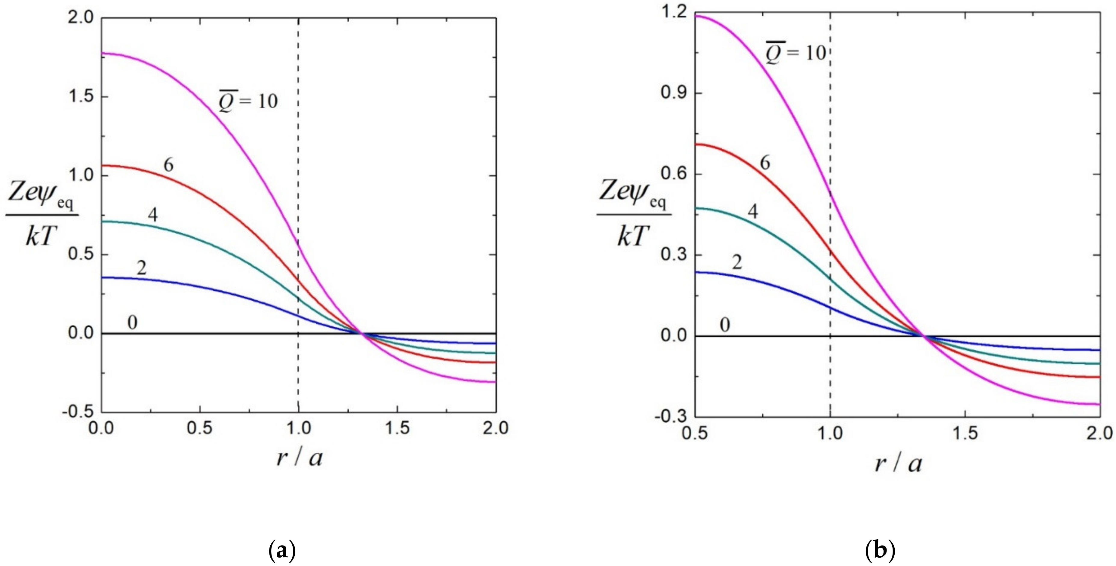
3.1. Equilibrium Electrostatic Potential

The equilibrium electrostatic potential distribution ${\psi }_{\mathrm{eq}}(r)$ inside a unit cell for a suspension of charged soft spheres in a salt-free solution is given by Equations (5) and (6). In Figure 2a,b, the dimensionless electric potential $Ze{\psi }_{\mathrm{eq}}/kT$ is plotted versus the scaled coordinate $r/a$ around a porous sphere ($r_0=0$) and a soft sphere with $r_0/a=1/2$, respectively, for various values of the scaled fixed charge density $\overline{Q}$ of the particles in the case of the particle volume fraction $\phi ={(a/b)}^3=0.125$. For specified values of $\overline{Q}$ and $\phi$, as expected, the value of $Ze{\psi }_{\mathrm{eq}}/kT$ is positive near the center of the porous particle and the hard-core surface of the soft particle, decreases monotonically with an increase in $r/a$ (especially in the vicinity of the particle surface), and becomes negative after a critical value of $r/a$, which corresponds to $n_{\mathrm{av}}$ for the local counterionic concentration and is a weak decreasing function of $\phi$ and $\overline{Q}$. The values of ${\psi }_{\mathrm{eq}}(r_0)$, $-{\psi }_{\mathrm{eq}}(b)$, ${\psi }_{\mathrm{eq}}(r_0)-{\psi }_{\mathrm{eq}}(r)$, and ${\psi }_{\mathrm{eq}}(r)-{\psi }_{\mathrm{eq}}(b)$ (where $r_0<r<b$) are greater for a soft sphere with a smaller value of the core-to-particle radius ratio $r_0/a$ (i.e., greatest for a porous sphere) and increase with an increase in $\overline{Q}$ from zero at $\overline{Q}=0$, keeping the other parameters unchanged.

The values of the dimensionless relative surface potential $Ze{\psi }_{\mathrm{s}}/kT$ for a charged porous sphere ($r_0=0$) and a charged soft sphere with $r_0/a=4/5$ in their corresponding salt-free suspensions calculated from Equation (10) are plotted versus the scaled fixed charge density $\overline{Q}$ in Figure 3a,b, respectively, for various values of $\phi$. As expected, ${\psi }_{\mathrm{s}}$ (or ${\psi }_{\mathrm{eq}}(r_0)$ or $-{\psi }_{\mathrm{eq}}(b)$) for a constant value of $\overline{Q}$ decreases with an increase in $\phi$ (i.e., a decrease in the relative cell size) and the effect of interactions among the particles in the suspensions on ${\psi }_{\mathrm{s}}$ or ${\psi }_{\mathrm{eq}}$ is significant. Note that, if $\overline{Q}$ is relatively high, our results obtained with the Debye–Hückel approximation may not apply for the salt-free suspensions with a low $\phi$, since in this case the electric potential becomes high because of the presence of very small amount of ions. When $\overline{Q}$ is small (say, $\overline{Q}\le 10$, which corresponds to $Ze{\psi }_{\mathrm{s}}/kT<0.95$ for $\phi \ge 0.1$), $Ze{\psi }_{\mathrm{s}}/kT$ is nearly proportional to $\overline{Q}$. When $\overline{Q}$ is relatively high, however, the increase of $Ze{\psi }_{\mathrm{s}}/kT$ with $\overline{Q}$ is somewhat suppressed due to the counterion condensation occurring near the fixed charges of the particles (which is obviously underestimated with the linearized Poisson–Boltzmann equation for obtaining Equations (5) and (6)). For fixed values of $\overline{Q}$ and $\phi$, the value of $Ze{\psi }_{\mathrm{s}}/kT$ for a soft sphere decreases with an increase in the core-to-particle radius ratio $r_0/a$ from $r_0/a=0$ (a porous sphere).

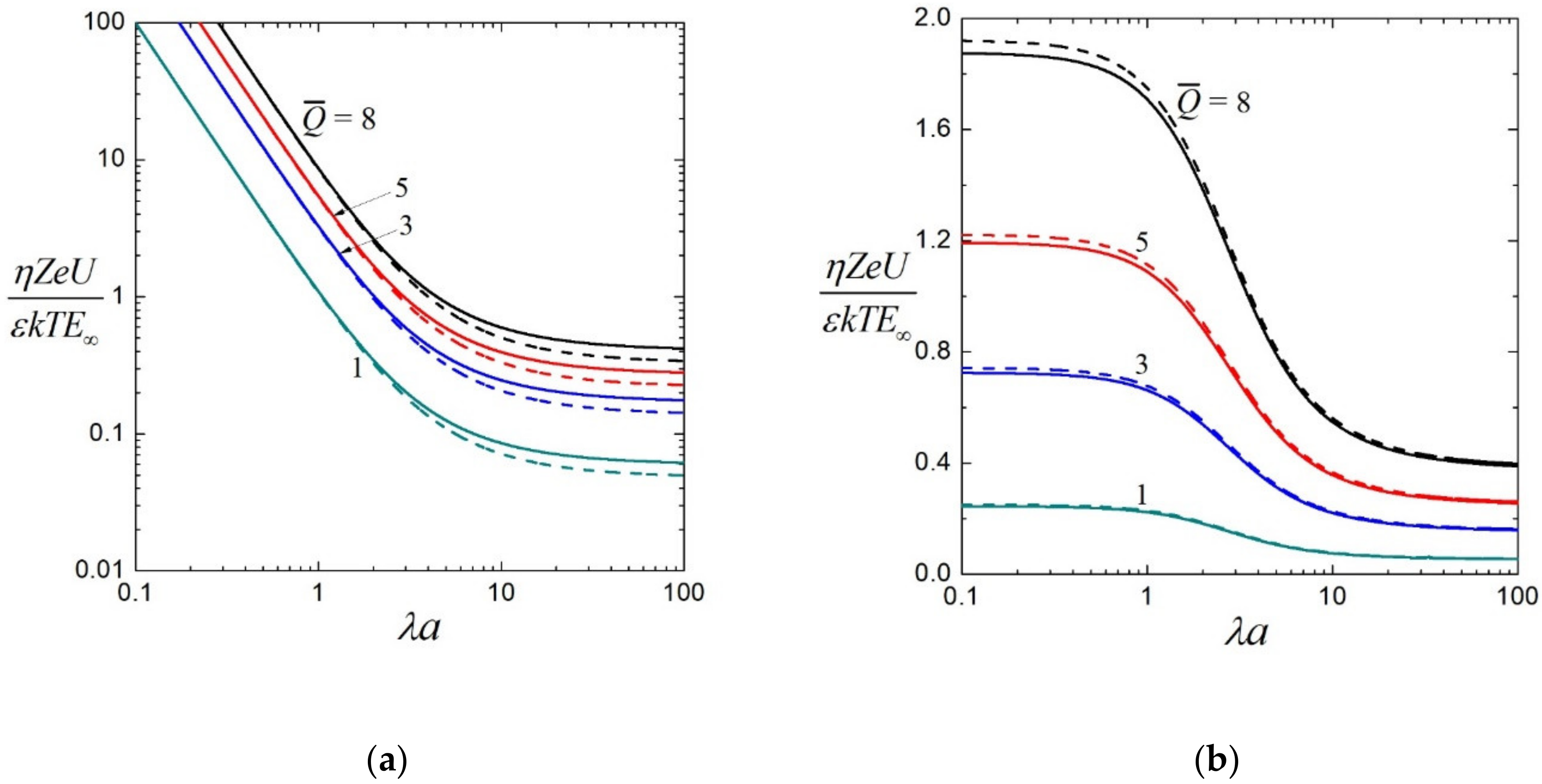
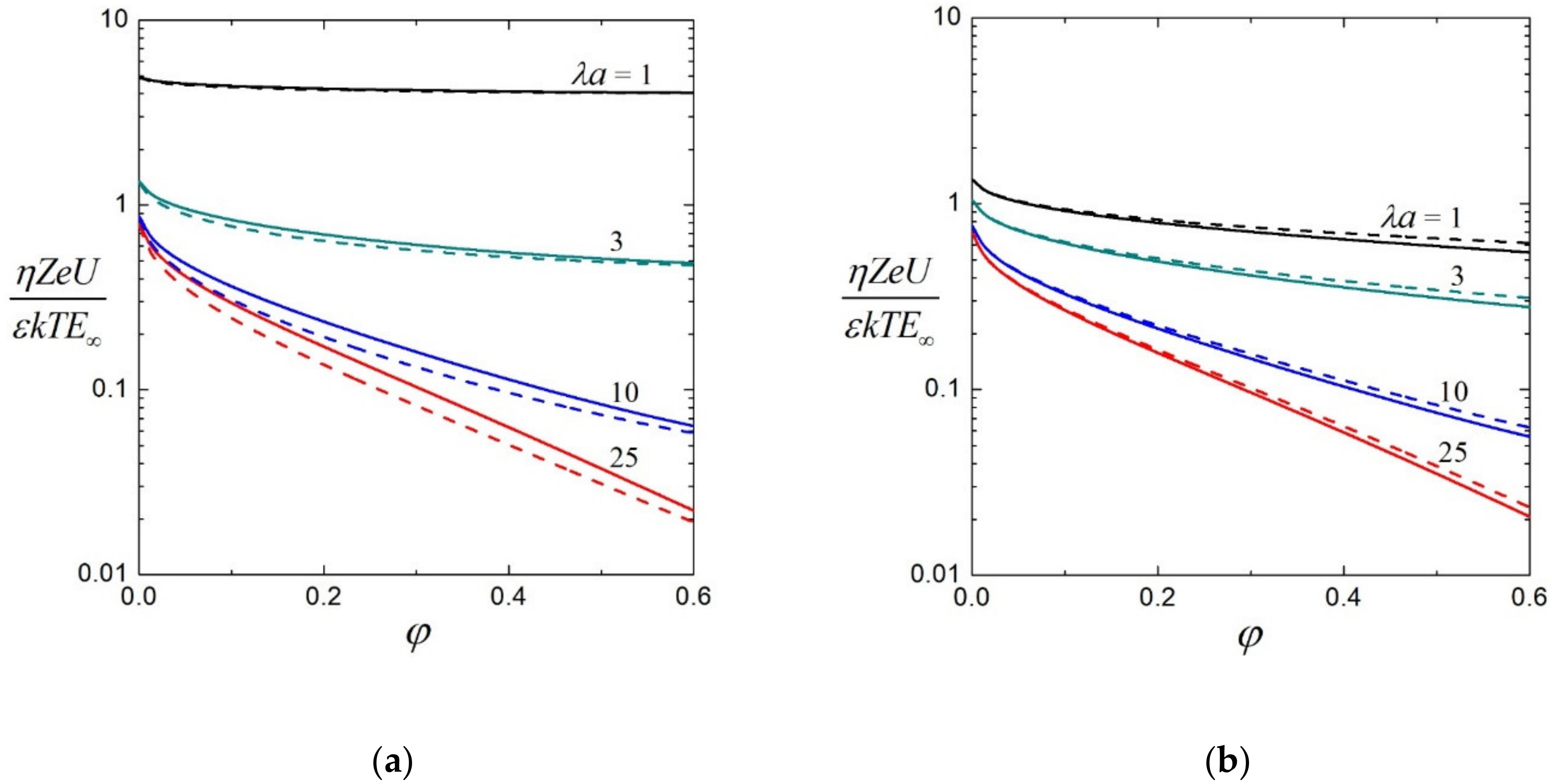
3.2. Electrophoretic Mobility

The scaled electrophoretic mobility $\eta ZeU/\epsilon kT{E}_{\infty }$ in a bounded salt-free suspension of charged soft spheres, calculated from Equation (45) for the Happel and Kuwabara models, is plotted versus the scaled fixed charge density $\overline{Q}$, shielding parameter $\lambda a$, particle volume fraction $\phi$, and core-to-particle radius ratio $r_0/a$ in Figure 4, Figure 5, Figure 6 and Figure 7, respectively. For the case of porous spheres ($r_0=0$), the coefficient $\nu$ in Equation (45) equals unity, independent of the boundary condition (13) or (14) for the external electric potential applied at the border of the unit cell. Consistent with the previous results [22,25] without the relaxation effect, $\eta ZeU/\epsilon kT{E}_{\infty }$ increases substantially with an increase in $\overline{Q}$, a decrease in $\lambda a$, a decrease in $\phi$, and a decrease in $r_0/a$, keeping the other parameters unchanged. Additionally, $\eta ZeU/\epsilon kT{E}_{\infty }$ is nearly proportional to $\overline{Q}$ as $\overline{Q}\le 10$ and its increase with $\overline{Q}$ is somewhat suppressed due to the counterion condensation effect (which is underestimated again with the Debye–Hückel approximation) when the value of $\overline{Q}$ is relatively high. For fixed values of $\overline{Q}$, $\lambda a$, $r_0/a$, and $\phi$, the Kuwabara model leads to a less value of $\eta ZeU/\epsilon kT{E}_{\infty }$ than the Happel model does, and the Neumann condition for the electrostatic potential at the outer boundary of the unit cell results in a greater value of $\eta ZeU/\epsilon kT{E}_{\infty }$ than the Dirichlet condition does, but both differences are unsubstantial.

For comparison with the case of a suspension containing added electrolytes, $\eta U/a^{2}Q{E}_{\infty }$ (or $\eta {\kappa }^{2}U/Q{E}_{\infty }$ or $\eta {\lambda }^{2}U/Q{E}_{\infty }$), the electrophoretic mobility of the salt-free suspension of soft spheres normalized with the fixed charge density $Q$ in the porous surface layer can be plotted versus the parameters $\kappa a$, $\lambda a$, $r_0/a$, and $\phi$. These figures, in which the value of $\eta U/a^{2}Q{E}_{\infty }$ decreases monotonically with increases in $\kappa a$, $\lambda a$, $r_0/a$, and $\phi$, are the same as those for a salt-containing suspension under the Debye–Hückel approximation [12,13,30].

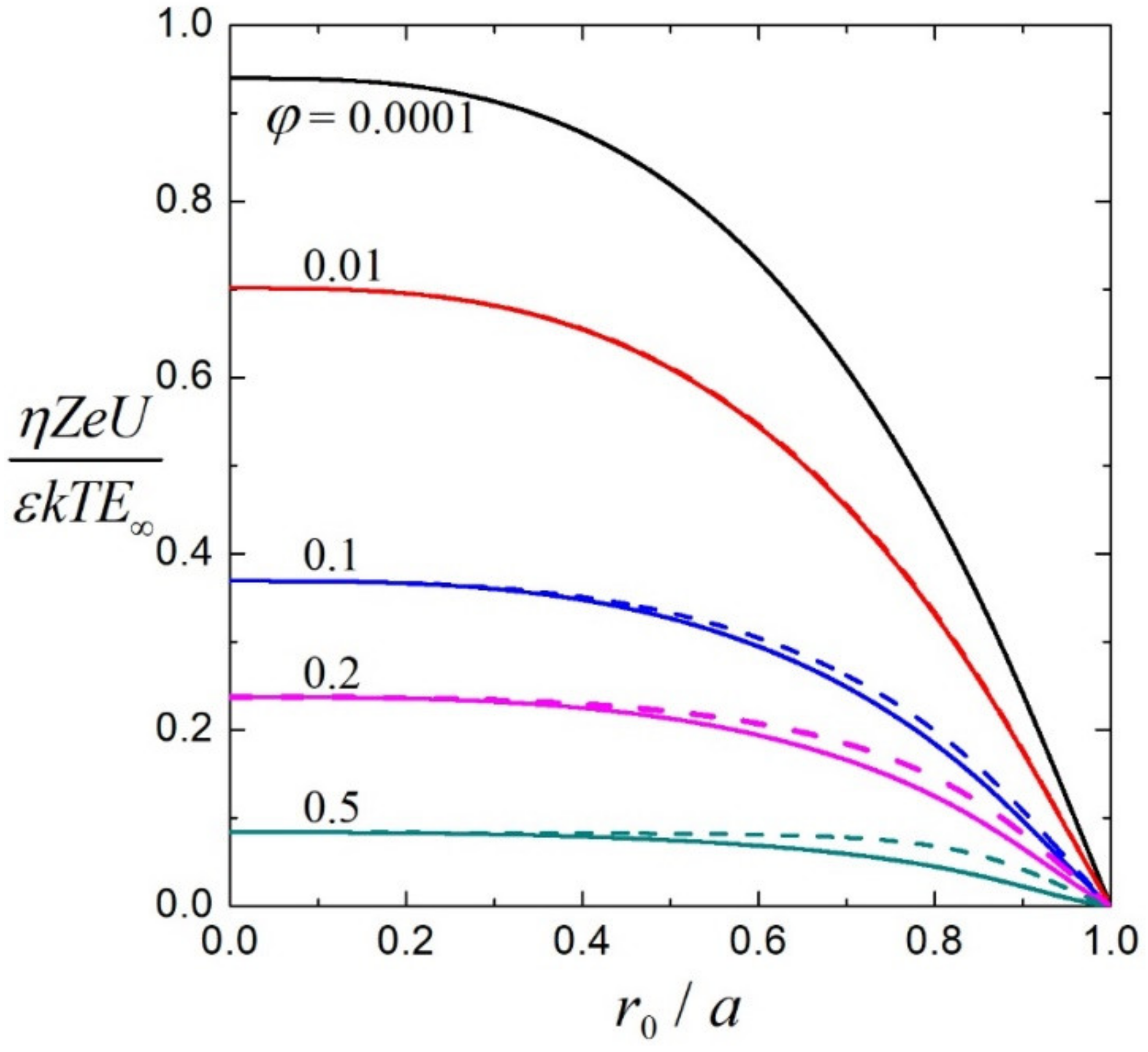
3.3. Effective Electric Conductivity

The normalized effective electric conductivity $\Lambda /{\Lambda }^{\infty }$ of a salt-free suspension of charged soft spheres calculated using Equation (47) is plotted versus the particle volume fraction $\phi$ and core-to-particle radius ratio $r_0/a$ in Figure 8 and Figure 9, respectively. The effect of particle interactions on the effective conductivity is significant. For a specified value of $\phi$, $\Lambda /{\Lambda }^{\infty }$ is a monotonic increasing function of the scaled fixed charge density $\overline{Q}$ and almost proportional to $\overline{Q}$ as $\overline{Q}\le 10$. For a given value of $\overline{Q}$, $\Lambda /{\Lambda }^{\infty }$ first increases with an increase in $\phi$, attains a maximum, and then decreases with a further increase in $\phi$. This behavior is different from that for the effective conductivity of a salt-containing suspension of charged soft spheres, where $\Lambda /{\Lambda }^{\infty }$ (with ${\Lambda }^{\infty }$ being the electric conductivity of the ionic solution in the absence of particles) as a function of $\phi$ depends on the valence, diffusivity, and bulk concentration of each ionic species [12,13]. For fixed values of $\overline{Q}$ and $\phi$, the value of $\Lambda /{\Lambda }^{\infty }$ decreases with an increase in $r_0/a$ from $r_0/a=0$ (porous spheres). Note that $\Lambda /{\Lambda }^{\infty }$ can be less than unity when $\overline{Q}$ is small, $\phi$ is large, and $r_0/a$ is large.

4. Summary

The electrophoresis and electric conduction of a salt-free suspension of charged soft spheres with arbitrary values of the particle volume fraction $\phi$, core-to-particle radius ratio $r_0/a$, and shielding parameter $\lambda a$ are analyzed by using a unit cell model in this work. Each soft sphere reduces to an entirely porous sphere if its hard core vanishes. The linearized Poisson–Boltzmann equation is solved for the equilibrium electric potential profile in the fluid containing the counterions only around the particle in a unit cell, and the counterionic continuity equation and modified Stokes/Brinkman equations are solved for the ionic electrochemical potential energy and fluid velocity distributions, respectively. Closed-form expressions for the electrophoretic velocity of the suspended particles with a low value of the scaled fixed charge density $\overline{Q}$ and the effective electric conductivity of the suspension are obtained in Equations (45) and (47), respectively. The effect of particle interactions on these transport characteristics is significant. Same as the case in a salt-containing suspension under the Debye–Hückel approximation, the scaled electrophoretic mobility in a salt-free suspension is a monotonic increasing function of $\overline{Q}$ and decreases with increases in $r_0/a$, $\lambda a$, and $\phi$, keeping the other parameters unchanged. The normalized effective electric conductivity of the salt-free suspension also increases with an increase in $\overline{Q}$ and with a decrease in $r_0/a$, but is not a monotonic function of $\phi$.

References

1. Levine, S.; Neale, G.H. The Prediction of Electrokinetic Phenomena within Multiparticle Systems I. Electrophoresis and Electroosmosis. J. Colloid Interface Sci. 1974, 47, 520–529. [Google Scholar] [CrossRef]
2. O’Brien, R.W. The Electric Conductivity of a Dilute Suspension of Charged Particles. J. Colloid Interface Sci. 1981, 81, 234–248. [Google Scholar] [CrossRef]
3. Zharkikh, N.I.; Shilov, V.N. Theory of Collective Electrophoresis of Spherical Particles in the Henry Approximation. Colloid J. USSR (Eng. Transl.) 1982, 43, 865–870. [Google Scholar]
4. Ohshima, H.; Healy, T.W.; White, L.R. Approximate Analytic Expressions for the Electrophoretic Mobility of Spherical Colloidal Particles and the Conductivity of Their Dilute Suspensions. J. Chem. Soc. Faraday Trans. 2 1983, 79, 1613–1628. [Google Scholar] [CrossRef]
5. Chen, S.B.; Keh, H.J. Axisymmetric Electrophoresis of Multiple Colloidal Spheres. J. Fluid Mech. 1992, 238, 251–276. [Google Scholar] [CrossRef]
6. Liu, Y.C.; Keh, H.J. Electric Conductivity of a Dilute Suspension of Charged Composite Spheres. Langmuir 1998, 14, 1560–1574. [Google Scholar] [CrossRef]
7. Ohshima, H. Electrical Conductivity of a Concentrated Suspension of Spherical Colloidal Particles. J. Colloid Interface Sci. 1999, 212, 443–448. [Google Scholar] [CrossRef]
8. Borkovec, M.; Behrens, S.H.; Semmler, M. Observation of the Mobility Maximum Predicted by the Standard Electrokinetic Model for Highly Charged Amidine Latex Particles. Langmuir 2000, 16, 5209–5212. [Google Scholar] [CrossRef]
9. Ding, J.M.; Keh, H.J. The Electrophoretic Mobility and Electric Conductivity of a Concentrated Suspension of Colloidal Spheres with Arbitrary Double-Layer Thickness. J. Colloid Interface Sci. 2001, 236, 180–193. [Google Scholar] [CrossRef] [Green Version]
10. Carrique, F.; Cuquejo, J.; Arroyo, F.J.; Jimenez, M.L.; Delgado, Á.V. Influence of Cell-Model Boundary Conditions on the Conductivity and Electrophoretic Mobility of Concentrated Suspensions. Adv. Colloid Interface Sci. 2005, 118, 43–50. [Google Scholar] [CrossRef]
11. Zholkovskij, E.K.; Masliyah, J.H.; Shilov, V.N.; Bhattacharjee, S. Electrokinetic Phenomena in Concentrated Disperse Systems: General Problem Formulation and Spherical Cell Approach. Adv. Colloid Interface Sci. 2007, 134–135, 279–321. [Google Scholar] [CrossRef] [PubMed]
12. Keh, H.J.; Liu, C.P. Electric Conductivity and Electrophoretic Mobility in Suspensions of Charged Porous Spheres. J. Phys. Chem. C 2010, 114, 22044–22054. [Google Scholar] [CrossRef]
13. Liu, H.C.; Keh, H.J. Electrophoresis and Electric Conduction in a Suspension of Charged Soft Spheres. Colloid Polym. Sci. 2016, 294, 1129–1141. [Google Scholar] [CrossRef]
14. Galli, M.; Sáringer, S.; Szilágyi, I.; Trefalt, G. A Simple Method to Determine Critical Coagulation Concentration from Electrophoretic Mobility. Colloids Interfaces 2020, 4, 20. [Google Scholar] [CrossRef]
15. Lin, W.C.; Keh, H.J. Diffusiophoresis in Suspensions of Charged Soft Particles. Colloids Interfaces 2020, 4, 30. [Google Scholar] [CrossRef]
16. Lai, Y.C.; Keh, H.J. Transient Electrophoresis of a Charged Porous Particle. Electrophoresis 2020, 41, 259–265. [Google Scholar] [CrossRef]
17. Delgado, Á.V.; Carrique, F.; Roa, R.; Ruiz-Reina, E. Recent Developments in Electrokinetics of Salt-Free Concentrated Suspensions. Curr. Opin. Colloid Interface Sci. 2016, 24, 32–43. [Google Scholar] [CrossRef]
18. Ohshima, H. Ion Size Effect on Counterion Condensation around a Spherical Colloidal Particle in a Salt-Free Medium Containing Only Counterions. Colloid Polym. Sci. 2018, 296, 1293–1300. [Google Scholar] [CrossRef]
19. Su, Y.W.; Keh, H.J. Electrokinetic Flow of Salt-Free Solutions in a Fibrous Porous Medium. J. Phys. Chem. B 2019, 123, 9724–9730. [Google Scholar] [CrossRef]
20. Ohshima, H. Electrophoretic Mobility of a Spherical Colloidal Particle in a Salt-Free Medium. J. Colloid Interface Sci. 2002, 248, 499–503. [Google Scholar] [CrossRef]
21. Ohshima, H. Electrokinetic Phenomena in a Dilute Suspension of Spherical Colloidal Particles in a Salt-Free Medium. Colloids Interfaces A 2003, 222, 207–211. [Google Scholar] [CrossRef]
22. Ohshima, H. Electrophoretic Mobility of a Soft Particle in a Salt-Free Medium. J. Colloid Interface Sci. 2004, 269, 255–258. [Google Scholar] [CrossRef]
23. Carrique, F.; Ruiz-Reina, E.; Arroyo, F.J.; Delgado, Á.V. Cell Model of the Direct Current Electrokinetics in Salt-Free Concentrated Suspensions: The Role of Boundary Conditions. J. Phys. Chem. B 2006, 110, 18313–18323. [Google Scholar] [CrossRef] [PubMed] [Green Version]
24. Chiang, C.-P.; Lee, E.; He, Y.-Y.; Hsu, J.-P. Electrophoresis of a Spherical Dispersion of Polyelectrolytes in a Salt-Free Solution. J. Phys. Chem. B 2006, 110, 1490–1498. [Google Scholar] [CrossRef] [PubMed]
25. He, Y.-Y.; Wu, E.; Lee, E. Electrophoresis in Suspensions of Charged Porous Spheres in Salt-Free Media. Chem. Eng. Sci. 2010, 65, 5507–5516. [Google Scholar] [CrossRef]
26. Luo, R.H.; Keh, H.J. Electrophoresis and electric conduction in a salt-free suspension of charged particles. Electrophoresis 2021, 42. [Google Scholar] [CrossRef]
27. Kong, C.Y.; Muthukumar, M. Monte Carlo study of adsorption of a polyelectrolyte onto charged surfaces. J. Chem. Phys. 1998, 109, 1522. [Google Scholar] [CrossRef]
28. Hierrezuelo, J.; Szilagyi, I.; Vaccaro, A.; Borkovec, M. Probing Nanometer-Thick Polyelectrolyte Layers Adsorbed on Oppositely Charged Particles by Dynamic Light Scattering. Macromolecules 2010, 43, 9108–9116. [Google Scholar] [CrossRef]
29. Lin, W.-C. Electrophoresis and Electric Conduction in Salt-Free Suspensions of Charged Soft Particles. Master’s Thesis, National Taiwan University, Taipei, Taiwan, 2021. [Google Scholar]
30. Keh, H.J.; Chen, W.C. Sedimentation Velocity and Potential in Concentrated Suspensions of Charged Porous Spheres. J. Colloid Interface Sci. 2006, 296, 710–720. [Google Scholar] [CrossRef]
Figure 1. Geometrical sketch for the electrophoresis of a soft sphere in a unit cell for a suspension.
Colloids 05 00045 g001
Figure 2. Dimensionless equilibrium electric potential Z e ψ eq / k T for a soft sphere in a unit cell of φ = 0.125 ( a / b = 0.5 ) versus the scaled coordinate r / a with Q ¯ as a parameter: (a) r 0 / a = 0 (porous sphere); (b) r 0 / a = 1 / 2 .
Colloids 05 00045 g002
Figure 3. Dimensionless relative surface potential Z e ψ s / k T for a suspension of soft spheres versus Q ¯ with φ as a parameter: (a) r 0 / a = 0 (porous spheres); (b) r 0 / a = 4 / 5 .
Colloids 05 00045 g003
Figure 4. Scaled electrophoretic mobility η Z e U / ε k T E versus Q ¯ for a suspension of soft spheres with λ a = 10 : (a) r 0 / a = 0 (porous spheres) with the solid and dashed curves representing calculations for the Happel and Kuwabara models, respectively; (b) φ = 0.125 for the Happel model with the solid and dashed curves denoting results obtained from conditions (13) and (14), respectively, at the cell border.
Colloids 05 00045 g004
Figure 5. Scaled electrophoretic mobility η Z e U / ε k T E versus λ a for a suspension of soft spheres with φ = 0.125 : (a) r 0 / a = 0 (porous spheres) with the solid and dashed curves representing calculations for the Happily and Kuwabara models, respectively; (b) r 0 / a = 1 / 2 for the Happel model with the solid and dashed curves denoting results obtained from conditions (13) and (14), respectively, at the cell border.
Colloids 05 00045 g005
Figure 6. Scaled electrophoretic mobility η Z e U / ε k T E versus φ for a suspension of soft spheres with Q ¯ = 4 : (a) r 0 / a = 0 (porous spheres) with the solid and dashed curves representing calculations for the Happel and Kuwabara models, respectively; (b) r 0 / a = 1 / 2 for the Happel model with the solid and dashed curves denoting results obtained from conditions (13) and (14), respectively, at the cell border.
Colloids 05 00045 g006
Figure 7. Scaled electrophoretic mobility η Z e U / ε k T E versus r 0 / a for a suspension of soft spheres with Q ¯ = 4 , λ a = 10 , and φ as a parameter for the Happel model. The solid and dashed curves denote results obtained from conditions (13) and (14), respectively, at the cell border.
Colloids 05 00045 g007
Figure 8. Normalized effective electric conductivity Λ / Λ versus φ with Q ¯ as a parameter for a suspension of soft spheres: (a) r 0 / a = 0 (porous spheres); (b) r 0 / a = 1 / 2 with the solid and dashed curves denoting results obtained from conditions (13) and (14), respectively, at the cell border.
Colloids 05 00045 g008
Figure 9. Normalized effective electric conductivity Λ / Λ versus r 0 / a for a suspension of soft spheres with Q ¯ = 4 and φ as a parameter. The solid and dashed curves denote results obtained from conditions (13) and (14), respectively, at the cell border.
Colloids 05 00045 g009
Publisher’s Note: MDPI stays neutral with regard to jurisdictional claims in published maps and institutional affiliations.