
Performance of UAV-to-Ground FSO Communications with APD and Pointing Errors


Department of Aerospace Electronics, School of Electronics and Telecommunications, Hanoi University of Science and Technology, Hanoi 100000, Vietnam
Appl. Syst. Innov. 2021, 4(3), 65; https://doi.org/10.3390/asi4030065
Submission received: 26 June 2021
/
Revised: 2 September 2021
/
Accepted: 3 September 2021
/
Published: 8 September 2021
(This article belongs to the Section Information Systems)
Abstract
:Recently, a combination of unmanned aerial vehicles (UAVs) and free-space optics (FSO) has been investigated as a potential method for high data-rate front-haul communication links. The aim of this work was to address the performance of UAV-to-ground station-based FSO communications in terms of the symbol error rate (SER). The system proposes utilizing subcarrier intensity modulation and an avalanche photo-diode (APD) to combat the joint effects of atmospheric turbulence conditions and pointing error due to the UAV’s fluctuations. In the proposed system model, the FSO transmitter (Tx) is mounted on the UAV flying over the monitoring area, whereas the FSO receiver (Rx) is placed on either the ground or top of a high building. Unlike previous works related to this topic, we considered combined channel parameters that affect the system performance such as transmitted power, link loss, various atmospheric turbulence conditions, pointing error loss, and the total noise at the APD receiver. Numerical results have shown that, for the best system SER performance, the value of an average APD gain at the Rx can be selected, varying from 18 to 30, whereas the equivalent beam waist radius at the Tx should be in a range from 2 to 2.2 cm in order to decrease the effects from the UAV’s fluctuations.
1. Introduction
Previously, unmanned aerial vehicles (UAVs), also known as drones, were mainly used in the military field. However, with the current industrial revolution, the application of new advances in information and communication technologies in traditional industrial fields is becoming significantly more commonplace. Since, AUVs have gradually become more popular, and are now being used more widely for civil purposes, especially in the fields of industry, agriculture, forestry, television, as well as applications in the field of space geoengineering [1,2,3]. Their costs are decreasing while providing greater efficiency. Specifically, a UAV can move to complex locations or notify areas that may pose danger to humans, and move steadily over the desired area to act as a relay node for communication cooperation between ground nodes and a central point (CP) [4,5].
In these cases, free-space optical (FSO) communications, a cost-effective, license-free, easy-to-deploy, high-bandwidth, and secure access technique, is being viewed as a potential candidate for the front-hauling transmission of multimedia data collected by flying UAVs from the CP [6,7,8,9,10,11]. For these reasons, FSO communication technology was naturally incorporated with UAV technology in order to establish high-speed optical communication networks in ground-to-air, air-to-ground, and air-to-air situations. However, one of the serious degradations to the performance of UAV-based FSO communications is the effect of perturbative conditions caused by refractive index changes due to temperature inhomogeneities and fluctuations in the pressure dynamics in the air path of the laser beam [12,13,14]. Another important factor is the oscillation of the UAV’s wobble during flight which results in a displacement deviation of the pointing error [15]. These lead to radiative fluctuations in the received signal, which severely degrades the performance of this communication system.
UAV-based FSO communication links have been relatively well studied in the literature [6,7,15,16,17,18,19]. In particular, the author in [6] proposed an approach of flying platforms for relaying the FSO backhaul or front-haul data traffic from the access-to-core networks. It can be considered as a promising solution for the 5G+ cellular network. In [7], a novel FSO front-haul channel model for a UAV-based system was developed by qualifying the geometric and misalignment losses. Moreover, the authors in [15] derived accurate statistical channel models for multi-roto UAV-based FSO communication links considering the combined effect of atmospheric turbulence along with the UAV’s angle-of-arrival (AoA) fluctuations. In addition, the authors in [16,17] studied multiple UAV-based FSO systems with beam pointing ability. For instance, in [16], Heng et al. adaptively studied beam divergence to reduce the parameters’ requirements, such as the receive aperture diameter, transmit power and pointing. In [17], Kaadan et al. designed a deterministic model and simulation platform for air-to-air FSO links to support multi-element optical transceiver arrays for different parameters (e.g., communication range, beam divergence, array size, beam wavelength, and platform dynamics). A tractable bit error rate (BER) expression for the FSO links based on UAV including the joint effects of the atmospheric turbulence channel together with pointing errors is provided in [18]. In [19], Mai et al. studied the effects of AoA variation and pointing error simultaneously to the airborne FSO system considering the adaptive beam size control technique. In [20], Wang et al. presented channel modeling, performance analysis, and parameter optimization for hovering UAV-based FSO communications. In the channel model for such a system, four types of impairments (i.e., atmospheric loss, atmospheric turbulence, pointing error and link interruption due to the angle of incidence oscillations) are considered.
However, most of these works were considered the channel modeling and have not taken into account the effects of Tx’s and Rx’s parameters on the system performance. Most recently, the authors in [21] suggested using APD at Rx to reduce the influence of UAV fluctuations in order to improve the performance of UAV-based FSO systems. The designed system employed an intensity modulation and direct detection (IM/DD) with on–off keying (OOK) modulation for evaluating the BER performance. In this paper, unlike previous works related to this topic, we propose using the APD receiver for the UAV-based FSO system considering subcarrier intensity quadrature amplitude modulation (SI-QAM). We derived and analyzed the system’s SER performance, taking into account the combined channel parameters such as transmitted power, link loss, various atmospheric turbulence conditions, pointing error loss and the total noise of the APD.
The rest of this paper is structured as follows. Section 2 describes the system and channel modeling. The SER analysis of the considered system over different atmospheric turbulence conditions and pointing error is presented in Section 3. Section 4 presents the numerical results to analyze the derived mathematical expressions of the system performance. Section 5 concludes this paper.
2. System and Channel Modeling
2.1. System Modeling
We consider a typical UAV-based FSO communication system with applications in the surveillance and monitoring of specific working environments, such as early natural disaster and environmental pollution detection: that of the water environment survey in estuarine and coastal environments, as depicted in Figure 1. The hovering UAV/drone navigates thanks to GNSS satellites for its positioning. The UAV communicates with the ground IoT sensor nodes via multiple-access RF when flying over cluster 1 and cluster 2 of the wireless sensor networks. The head node communicates with ground IoT nodes using any wireless connectivity, including short-range (e.g., Bluetooth, Z-wave), medium-range (e.g., Wi-Fi, ZigBee), and long-range (e.g., LoRa, NB-IoT) means. The UAV collects various data from ground surfaces such as environmental air and water data, captured images or videos recorded from monitoring cameras. In such scenarios, the UAV acts as a mobile gateway in the IoT network.
We also consider an FSO transmitter (Tx) mounted on the UAV/drone. The FSO Tx uses the SI-QAM to compensate for the limitations of the OOK and pulse-position modulation (PPM) schemes. Firstly, data collected from ground nodes will be used for electrical modulation to generate the electrical signal. The SIM modulates each block of data bits including -PAM symbols and -PAM symbols using the subcarrier in both in-phase () amplitude and quadrature amplitude () in the signal space. Then, the modulated signal is employed to modulate the intensity of the laser before transmitting toward to the Rx. Consequently, the transmitted optical signal can be formulated as [13]
where and m are the average transmitted power per symbol and the modulation index, respectively.
At the FSO Rx side, the received optical signal at the APD receiver can be obtained as [13]
where denotes the instantaneous turbulence channel of the FSO link that is the stationary random process of the optical signal scintillation, link loss, position and orientation fluctuation due to the hovering UAV. In Equation (2), the filter can be used for filtering out the component of . Consequently, the electrical signal received at the APD receiver output can be written as
where G and ℜ denote the average gain of the APD and responsivity (also called the quantum efficiency), respectively. is the total noise at the output of the APD including the in-phase and quadrature . They can be modeled as zero-mean Gaussian distribution with the assumption that the variance is the same. They can be expressed as
where , , and are the noise variance of the shot noise due to the desired received signal, the noise variance of thermal noise, and the noise variance due to undesired background radiation, respectively. Particularly, the depends on the average APD gain G, the excess noise factor F, the electrical bandwidth of the APD , and the average transmitted power . can be given by [22]
In Equation (5), where , , c, and e denote the Planck constant, the optical frequency, the speed of light and the electron charge, respectively. The thermal noise variance can be given by [22]
where , T, are the Boltzmann constant, Rx’s equivalent temperature in degrees Kelvin, and APD’s load resistance, respectively.
Moreover, as illustrated in Figure 2, the Rx lens accumulates the transmitted optical signal beam, which is projected onto the Rx plane’s surface. The incoming optical signal then converges onto the surface of the APD’s area. In this process, in addition to the desired optical signal, the background noise from the scattered sunlight is also added to the receiver. Therefore, because of the undesired background, the noise variance is obtained as
where represents the background power, which is generated by extended sources (e.g., the sky), r is the Rx lens radius, is the optical filter bandwidth at the Rx (), is the spectral radiance of the background radiations at the optical wavelength (Watt/cm2––srad), and is the Rx’s field-of-view (FOV) angle [15]. It is noted that is the lens area of the optical receiver (cm2).
Finally, the electrical signal-to-noise ratio (SNR) at the APD receiver output can be instantaneously formulated as
where X denotes the instantaneous channel coefficient. Because the atmospheric turbulence causes the slow fading nature of the scintillation process in the FSO link, the average symbol error rate (SER) is one of metrics for evaluating the performance of the considered system that employs the SI-QAM modulation. SER can be defined as
where denotes the distribution of X.
2.2. Channel Modeling
During the optical signal propagation from the UAV to FSO receiver over the atmospheric channel, the amplitudes and phases are distorted by different interferences such as absorption, scattering and refraction. In this study, we consider the combined effects of three primary parameters characterizing an UAV/FSO channel on the received signal intensity including (i) the atmospheric attenuation which causes the link loss ; (ii) the atmospheric turbulence causes random intensity fluctuation ; and (iii) the geometric and pointing error due to the UAV’s fluctuation . Hence, the combined channel coefficient X can be given by the following equation [7]
2.2.1. Atmospheric Attenuation and Turbulence
The atmospheric attenuation caused by both molecular absorption and aerosol scattering suspended in the air. The total link loss caused by the attenuation of can therefore be obtained as [23]
where L and are the transmission distance between the FSO Tx and the FSO Rx and the weather-dependent attenuation coefficient, respectively.
Considering the fading channel induced by atmospheric turbulence, we use the log-normal (LN) distribution model for the case of weak to moderate turbulence and the gamma–gamma (GG) distribution model for the case of moderate to strong turbulence. The probability density function (PDF) of the channel intensity fluctuation in the LN model can be expressed as [14]
where represents the scintillation index that depends on the channel’s characteristics and is expressed as [14]
where , is the Rytov variance. In the case of spherical wave propagation, it is given by [14]
In Equation (14), is the optical wave-number, (in ) denotes the index of the refraction structure parameter that represents the strength of the atmospheric turbulence, where is the operating height of the hovering UAV and is the nominal value of the refractive index at the ground [24]. In the practical system, the variance is very small. Therefore, is assumed to be altitude-dependent and constant along the propagation path, and typically takes values varying from to under atmospheric turbulence conditions, accordingly.
The Rytov variance distinguishes the various link turbulence regimes such as weak turbulence if , moderate turbulence if and strong turbulence if , especially saturated turbulence if .
On the other hand, the PDF distribution of the random variable in the GG model is given by [13]
2.2.2. Pointing Error Loss
We consider the Gaussian beam at the FSO Tx, and the pointing error-induced geometrical loss can be modeled as [24,25]
where is the distance of the beam sport shifted to the position of the receiver lens (see Figure 3). The parameter represents the maximal fraction of the collected intensity with , and r denotes the Rx lens radius, is the error function, denotes the equivalent beam waist at the distance y, with represents the beam waist radius of the Tx at , , and is the coherence length.
The center of the incoming optical beam is deviated from the center of the FSO Rx lens due to the random displacement of FSO Tx caused by the hovering UAV. On the other hand, the angle-of-arrival of the Tx optical signal can be explained as follows. As described in Figure 2, the Rx lens focus the incoming light onto the PD area using either APD or PIN photo-detectors in the (x, z) plane. The incidence angle relative to the Rx detector axis is denoted by . Hence, it is expressed as . Furthermore, it can be approximated as , which has a Rayleigh distribution as [18]
In Equation (19), denotes the variance of the , and represent the variances of the orientation deviations of the Tx and Rx, respectively.
Due to the limitations of Rx’s FOV and AoA fluctuations, a link interruption occurs for . We assume that the link loss takes two discrete values of “1” and “0”, corresponding to one of the symbols for the determination that the incoming optical signal was projected on the Rx’s FOV or not. Therefore, because of AoA fluctuations, the corresponding lost can be obtained by [15]
In Equation (20), if , otherwise . Moreover, the RV conditioned on and has a Rician distribution that can be represented as [18]
where is the modified Bessel function of the first kind with order zero. From (20) and (21), the distribution of can be derived as
where is the Dirac delta function and is defined as
Finally, the distribution of AoA fluctuation can be derived as
2.2.3. Combined Channel Models
The AoA fluctuation and orientation deviations of the FSO transmitter cause deviations to the center of the received beam at the FSO receiver plane, and the dependence of the RVs and are conditioned on the RV of the on the plane . Therefore, the PDF of X can be obtained as
where is the PDF of the RV x conditioned on the RV y, and:
Then, the completed statistical models of the UAV/FSO channel, considering the effect of link loss and atmospheric turbulence, the effective pointing error-induced geometrical loss can be derived.
In the first case of weak to moderate turbulence conditions, the log-normal model of the air-to-ground FSO communication links-based UAV has a PDF obtained as
where and is the well-known Q-function, and . Moreover, and are the variances of the position deviations of the Tx and Rx, respectively.
In the second case of moderate to strong atmospheric turbulence conditions, the GG model of the UAV-based air-to-ground FSO communication link has a PDF given as
3. Symbol Error Rate Calculation
This section studies the SER calculation of the above system in both weak and strong atmospheric turbulence channels, considering the pointing error and fluctuations from the FSO Tx mounted on the UAV to the FSO Rx.
The generalized ASER expression for evaluating the UAV-based FSO system over the LN and GG atmospheric fading channels can be expressed by
where represents the conditional error probability (CEP) and is the PDF of SNR, . By employing general –QAM constellations with two independent in-phase and quadrature signal amplitudes, the CEP is given by [13,25]
In the above equation, where , the Gaussian Q-function is defined by
where relates to the terms of the complementary error function . and which can be calculated from , are in-phase, quadrature distances. They are defined as , and in which
The SER is then calculated by
3.1. SER Calculation of Weak to Moderate Links
From Equations (27) and (33), the PDF of log-normal channels can be expressed for weak to moderate links as
The SER expression of the UAV-based FSO systems in cases of weak to moderate links can be derived as
3.2. SER Calculation of Moderate to Strong Links
From Equations (28) and (33), the PDFs and SER of the SNR for moderate to strong atmospheric turbulence can be derived as
Again, the SER expression of the UAV-based FSO systems in cases of moderate to strong links can be expressed as
4. Performance Results
In this section, we provide numerical results in terms of SER to analyze the performance of the UAV-to-ground FSO communication system with APD and pointing errors under the influence of various operating conditions. The subcarrier intensity QAM modulation scheme was employed in the evaluation. Table 1 provides the relevant parameters of the UAV-to-ground FSO communication system.
We considered using one UAV, under the assumption that the UAV hovers over a specific monitoring area to collect measured data from sensors on the ground. The UAV carries the payload of the FSO transmitter. In addition, an APD receiver-based FSO Rx station is located on the ground to collect data transmitted from the FSO transmitter mounted on the UAV. For the UAV and FSO Tx parameters, various typical system parameters are considered as follows. The optical operating wavelength , the beam waist radius from 0.3 to 0.08 m, the average transmitted power per symbol = −15 ÷ 5 dBm. Regarding the FSO link, the attenuation coefficient of = 3.436, and the turbulence strengths of m, m, and m for weak, moderate, and strong turbulence, respectively. For the FSO Rx parameters, we considered the system parameters as follows. The receiver aperture diameter of D = 0.08 m, the electrical bandwidth of APD = Hz, the Planck constant of = m Kg/s, the APD’s load resistance of = 1000 , the receiver noise temperature of T = 300 K, the ionization factor of = 0.7, the Boltzmann’s constant of = J/K, and the amplifier noise figure of = 2. Moreover, the variances in the orientation deviations of the Tx and Rx of = = 6 cm for the low UAV’s stability level, the variances of position deviations of the Tx and Rx of = = 30 cm [21].
Figure 4 plots the distribution comparison of the combined channel model with the channel model proposed in [15] for the case of a strong atmospheric turbulence channel, and the transmitter beam waist radius = 0.02 m. The combined channel distribution has higher density in the low region, resulting in a more unexpected impact on the system’s performance.
Figure 5 shows the SER-performance versus APD gain for various turbulence strengths of with the transmission link length of 800 m, and the average transmitted power per symbol of = −5 dBm. It can be seen that the SER-performance strongly depends on the weather-related turbulence conditions. In addition, when increasing the APD’s gain, the noise variances due to the desired received signal of and the undesired background radiation also increase, leading to decreased system SER performance. More importantly, it can also be seen that the selection of the APD’s gain, G, has a significant impact on the system performance. By using the derived SER expressions, the G’s values are converged on the optimal line for the minimal SER value. Specifically, to achieve the best systems’ SER-performance, the optimal gain value can be chosen in the range from 18 to 30. For example, with the weak atmospheric turbulence condition using G = 18, the system SER-performance can be approximately achieved at . However, with the strong atmospheric turbulence condition increasing G to 25, the system SER-performance will be approximately achieved at .
Then, Figure 6 provides the impact of the beam waist radius on the Tx to SER-performance for different values of turbulence strength and pointing error displacement standard deviations of = 0.05, 0.07, 0.1, with a transmission link length of 800 m and an APD’s gain D = 20. We found that the system performance strongly depends on this. It is highlighted in the results that by increasing the beam waist radius at the Tx to a proper value, the SER-performance of the specific APD receiver for all the pointing error displacement standard deviations decrease significantly. Then, the system-performance converge to the minimum of SER at the optimal value of . Consequently, would be selected for the best performance from 2 cm ÷ 2.2 cm operating under various system parameters. In addition, when increasing the value of from the optimal gain, the SER-performance steadily increases and progresses to saturation levels. For example, SER ≈ when ≥ 0.05 m for the system operating under moderate atmospheric turbulence conditions. This is reasonable because the higher the level of instability of the UAV is at the Tx, the wider the optical beam to reduce the influence of fluctuations on the Rx is.
Then, we investigate in Figure 7 the performance of a UAV-based FSO system versus the link distance L for, again, different values of turbulence strength and pointing error displacement standard deviations of = 0.05, 0.07, 0.1, using the optimal beam waist radius. As we can observe, the results from Figure 7 show that a decreasing L can compensate for the effects of UAV’s fluctuation on the system performance.
Finally, we show in Figure 8 the performance of the UAV-based FSO system versus the average electrical SNR for different QAM modulation schemes, e.g., 8-PSK and 16-QAM, with/without pointing error. The simulation was also performed for verifying the accuracy of the provided analytical expressions. The system included the weak to moderate atmospheric turbulence condition , G = 18. The link distance L = 800 m. The pointing error displacement standard deviation = 0.05, using the optimal beam waist radius = 0.02 m. It can be seen that, compared to there being no pointing errors, the SER with pointing errors significantly decreases the system performance. On the other hand, the use of a high-order modulation scheme leads to decreasing the achieved SER. For example, at the target BER = , the power gain of approximately 5 dB can be achieved when employing the 8-PSK scheme instead of the 16-QAM scheme.
5. Conclusions
In this paper, we analyzed the performance of a UAV FSO system employing subcarrier intensity QAM modulation and APD at the receiver under atmospheric turbulence conditions in the presence of pointing errors-induced geometrical loss. The SER analysis of the system was theoretically derived taking into account various parameters, linking atmospheric conditions and the pointing error effects. Then, we studied the performance of the considered system over different channel parameters due to UAV fluctuations. From analyzing the results of this study, using proper values of the beam waist radius and average APD gain could greatly benefit by compensating the influences of the UAV’s fluctuations on the performance of the system.
Funding
This research was funded by the Hanoi University of Science and Technology (HUST) under project number T2020-SAHEP-015.
Institutional Review Board Statement
Not applicable.
Informed Consent Statement
Not applicable.
Data Availability Statement
Data is contained within the article.
Conflicts of Interest
The author declares no conflict of interest.
References
- Chamola, V.; Kotesh, P.; Agarwal, A.; Naren; Gupta, N.; Guizani, M. A comprehensive review of unmanned aerial vehicle attacks and neutralization techniques. Ad. Hoc. Netw. 2021, 11, 102324. [Google Scholar] [CrossRef]
- Salhaoui, M.; Guerrero-González, A.; Arioua, M.; J Ortiz, F.; Oualkadi, A.E.; Torregrosa, C.L. Smart industrial IoT monitoring and control system based on UAV and cloud computing applied to a concrete plant. Sensors 2019, 19, 3316. [Google Scholar] [CrossRef] [Green Version]
- Hildmann, H.; Kovacs, E. Review: Using unmanned aerial vehicles (UAVs) as mobile sensing platforms (MSPs) for disaster response, civil security and public safety. Drones 2019, 3, 59. [Google Scholar] [CrossRef] [Green Version]
- Popescu, D.; Stoican, F.; Stamatescu, G.; Chenaru, O.; Ichim, L. A survey of collaborative UAV–WSN systems for efficient monitoring. Sensors 2019, 19, 4690. [Google Scholar] [CrossRef] [Green Version]
- Tien, P.V.; Nguyen, P.V.; Trung, H.D. Self-navigating UAVs for supervising moving objects over large-scale wireless sensor networks. Int. J. Aerosp. Eng. 2020, 2027340. [Google Scholar]
- Alzenad, M.; Shakir, M.Z.; Yanikomeroglu, H.; Alouini, M.-S. FSO-based vertical backhaul/fronthaul framework for 5G+ wireless networks. IEEE Commun. Mag. 2018, 56, 218–224. [Google Scholar] [CrossRef] [Green Version]
- Najafi, M.; Ajam, H.; Jamali, V.; Diamantoulakis, P.D.; Karagiannidis, G.K.; Schober, R. Statistical modeling of the FSO fronthaul channel for UAV-based communications. IEEE Trans. Commun. 2020, 68, 3720–3736. [Google Scholar] [CrossRef] [Green Version]
- Kurt, G.K.; Khoshkholgh, M.G.; Alfattani, S.; Ibrahim, A.; Darwish, T.S.J.; Alam, M.S.; Yanikomeroglu, H.; Yongacoglu, A. A vision and framework for the high altitude platform station (HAPS) networks of the future. IEEE Commun. Surv. Tutor. 2021, 23, 729–779. [Google Scholar] [CrossRef]
- Zhang, Y.; Wang, Y.; Deng, Y.; Du, A.; Liu, J. Design of a free space optical communication system for an unmanned aerial vehicle command and control link. Photonics 2021, 8, 163. [Google Scholar] [CrossRef]
- Fotouhi, A.; Qiang, H.; Ding, M.; Hassan, M.; Giordano, L.G.; Garcia-Rodriguez, A.; Yuan, J. Survey on UAV cellular communications: Practical aspects, standardization advancements, regulation, and security challenges. IEEE Commun. Surv. Tutor. 2019, 21, 3417–3442. [Google Scholar] [CrossRef] [Green Version]
- Ding, J.; Mei, H.; I, C.-L.; Zhang, H.; Liu, W. Frontier progress of unmanned aerial vehicles optical wireless technologies. Sensors 2020, 20, 5476. [Google Scholar] [CrossRef]
- Dautov, K.; Kalikulov, N.; Kizilirmak, R.C. The Impact of Various Weather Conditions on Vertical FSO Links. In Proceedings of the 2017 IEEE 11th International Conference on Application of Information and Communication Technologies (AICT), Moscow, Russia, 20–22 September 2017. [Google Scholar]
- Trung, H.D.; Tuan, D.T. Performance of free-space optical communications using SC-QAM signals over strong atmospheric turbulence and pointing errors. In Proceedings of the 2014 IEEE Fifth International Conference on Communications and Electronics (ICCE), Danang, Vietnam, 30 July–1 August 2014; pp. 42–47. [Google Scholar]
- Khalighi, M.A.; Uysal, M. Survey on free space optical communication: A communication theory perspective. IEEE Commun. Surv. Tutor. 2014, 16, 2231–2258. [Google Scholar] [CrossRef]
- Dabiri, M.T.; Sadough, S.M.S.; Khalighi, M.A. Channel modeling and parameter optimization for hovering UAV-based free-space optical links. IEEE J. Sel. Areas Commun. 2018, 36, 2104–2113. [Google Scholar] [CrossRef] [Green Version]
- Heng, K.H.; Liu, N.; He, Y.; Zhong, W.D.; Cheng, T.H. Adaptive Beam Divergence for Inter-UAV Free Space Optical Communications. In Proceedings of the 2008 IEEE PhotonicsGlobal@Singapore, Singapore, 8–11 December 2008; pp. 1–4. [Google Scholar]
- Kaadan, A.; Refai, H.H.; LoPresti, P.G. Multielement FSO transceivers alignment for inter-UAV communications. J. Lightw. Technol. 2014, 32, 4785–4795. [Google Scholar] [CrossRef]
- Dabiri, M.T.; Sadough, S.M.S.; Ansari, I.S. Tractable optical channel modeling between UAVs. IEEE Trans. Veh. Technol. 2019, 68, 11543–11550. [Google Scholar] [CrossRef]
- Mai, V.V.; Kim, H. Beam size optimization and adaptation for high-altitude airborne free-space optical communication systems. IEEE Photonics J. 2019, 11, 1–13. [Google Scholar] [CrossRef]
- Wang, J.-Y.; Ma, Y.; Lu, R.-R.; Wang, J.-B.; Lin, M.; Cheng, J. Hovering UAV-based FSO communications: Channel modelling, performance analysis, and parameter optimization. arXiv 2021, arXiv:2104.05368. [Google Scholar]
- Khankalantary, S.; Dabiri, M.T.; Safic, H. BER performance analysis of drone-assisted optical wireless systems with APD receiver. Optics Commun. 2020, 463, 1–7. [Google Scholar] [CrossRef]
- Trung, H.D.; Hoa, N.T.; Trung, N.H.; Ohtsuki, T. A Closed-form expression for performance optimization of subcarrier intensity QAM signals-based relay-added FSO systems with APD. Phys. Commun. J. 2018, 31, 203–211. [Google Scholar] [CrossRef]
- Karp, S.; Gagliardi, R.M.; Moran, S.E.; Stotts, L.B. Optical Channel: Fibers, Clouds, Water, and the Atmosphere; Springer: New York, NY, USA, 1988. [Google Scholar]
- AlQuwaiee, H.; Yang, H.-C.; Alouini, M.-S. On the asymptotic capacity of dual-aperture FSO systems with generalized pointing error model. IEEE Trans. Wilress Commun. 2016, 15, 6502–6512. [Google Scholar] [CrossRef] [Green Version]
- Ai, D.H.; Trung, H.D.; Tuan, D.T. On the ASER performance of amplify-and-forward relaying MIMO/FSO systems using SC-QAM signals over log-normal and gamma-gamma atmospheric turbulence channels and pointing error impairments. J. Inf. Telecommun. 2020, 4, 267–281. [Google Scholar] [CrossRef] [Green Version]
Figure 1.
A proposed UAV-based free-space optical communication system.
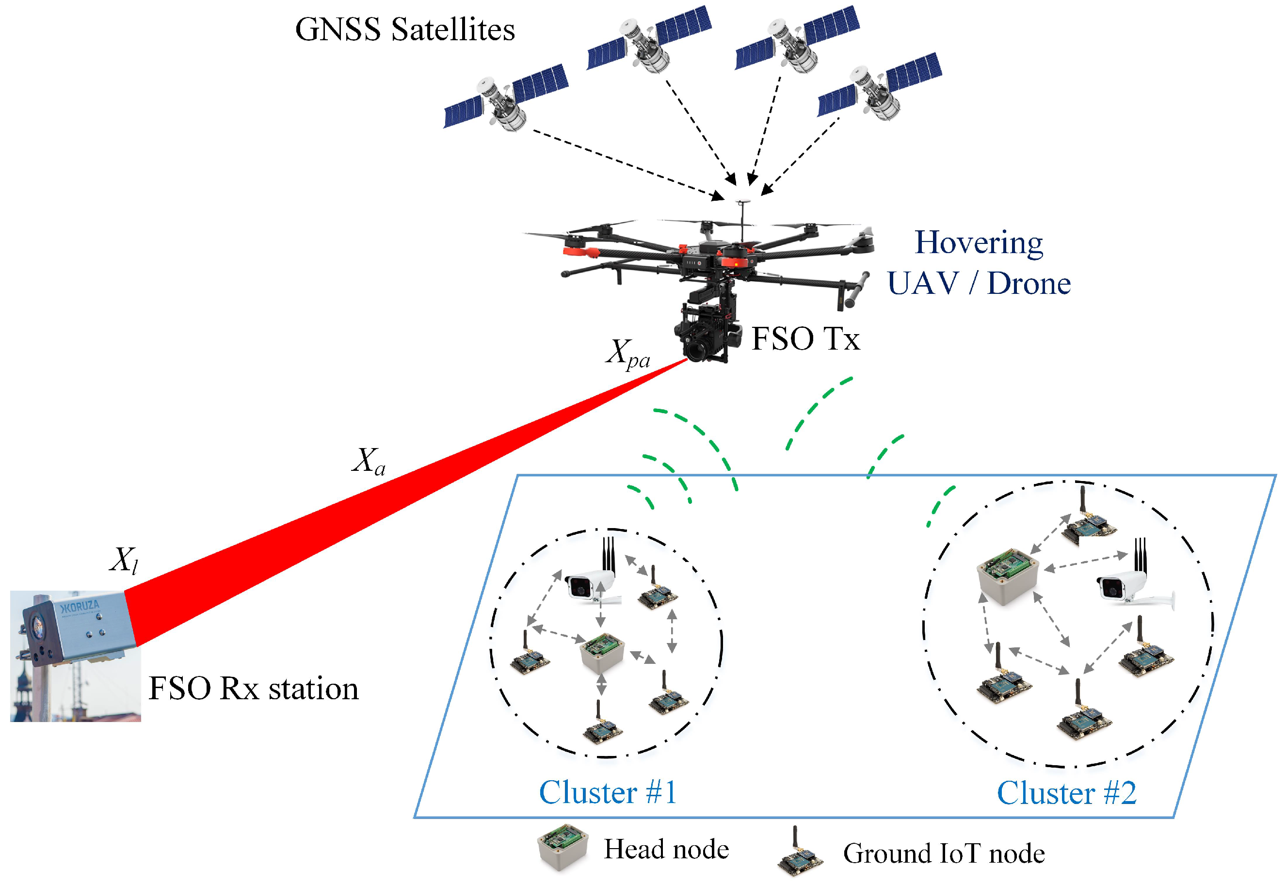
Figure 2.
Modeling of the received beam at the FSO Rx station in the presence of UAV’s fluctuations.
Figure 2.
Modeling of the received beam at the FSO Rx station in the presence of UAV’s fluctuations.

Figure 3.
Modeling the received beam at the FSO Rx station in the presence of fluctuations due to UAV hovering.
Figure 3.
Modeling the received beam at the FSO Rx station in the presence of fluctuations due to UAV hovering.
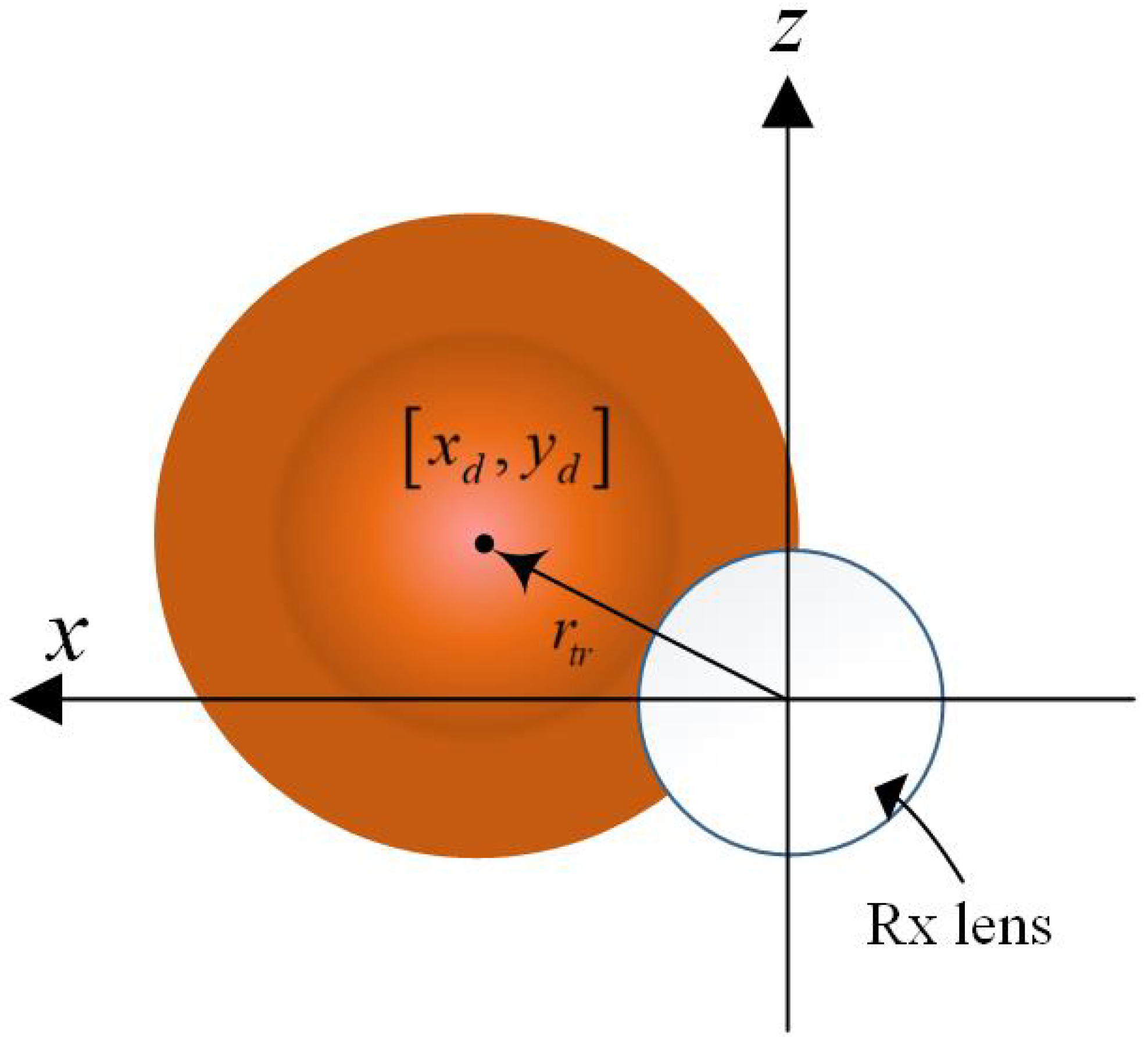
Figure 4.
The combined channel model distribution for the case of strong atmospheric turbulence channel, the transmitter beam waist radius = 0.02 m.
Figure 4.
The combined channel model distribution for the case of strong atmospheric turbulence channel, the transmitter beam waist radius = 0.02 m.

Figure 5.
SER versus APD gain, G, for different values of turbulence strength with a transmission link length of 800 m, an average transmitted power per symbol of = −5 dBm.
Figure 5.
SER versus APD gain, G, for different values of turbulence strength with a transmission link length of 800 m, an average transmitted power per symbol of = −5 dBm.

Figure 6.
SER versus beam waist radius, , for different values of turbulence strength with a transmission link length of 800 m, different values of turbulence strength and various values of the pointing error displacement standard deviation = 0.05, 0.07, and 0.1 (from bottom to top).
Figure 6.
SER versus beam waist radius, , for different values of turbulence strength with a transmission link length of 800 m, different values of turbulence strength and various values of the pointing error displacement standard deviation = 0.05, 0.07, and 0.1 (from bottom to top).
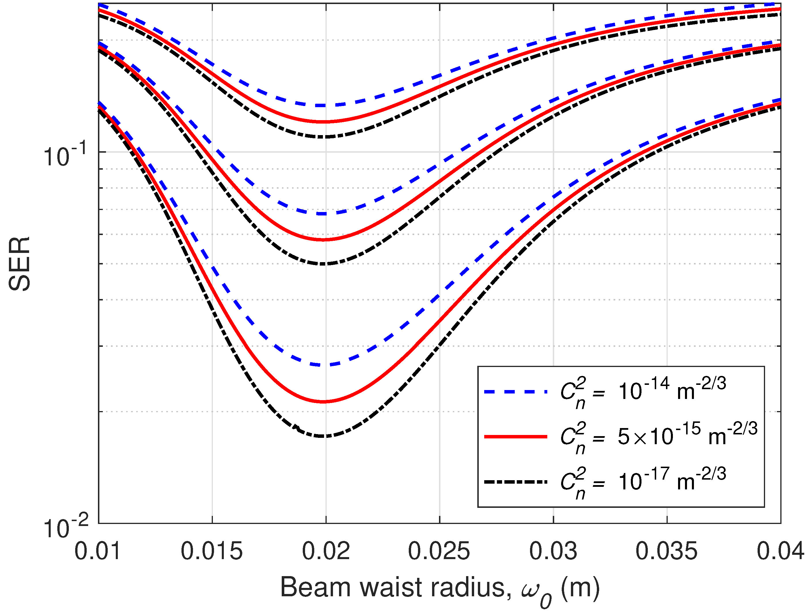
Figure 7.
SER versus link distance, L, for different values of turbulence strength, various values of the pointing error displacement standard deviation = 0.05, 0.07, and 0.1 (from bottom to top) with the optimal beam waist radius.
Figure 7.
SER versus link distance, L, for different values of turbulence strength, various values of the pointing error displacement standard deviation = 0.05, 0.07, and 0.1 (from bottom to top) with the optimal beam waist radius.
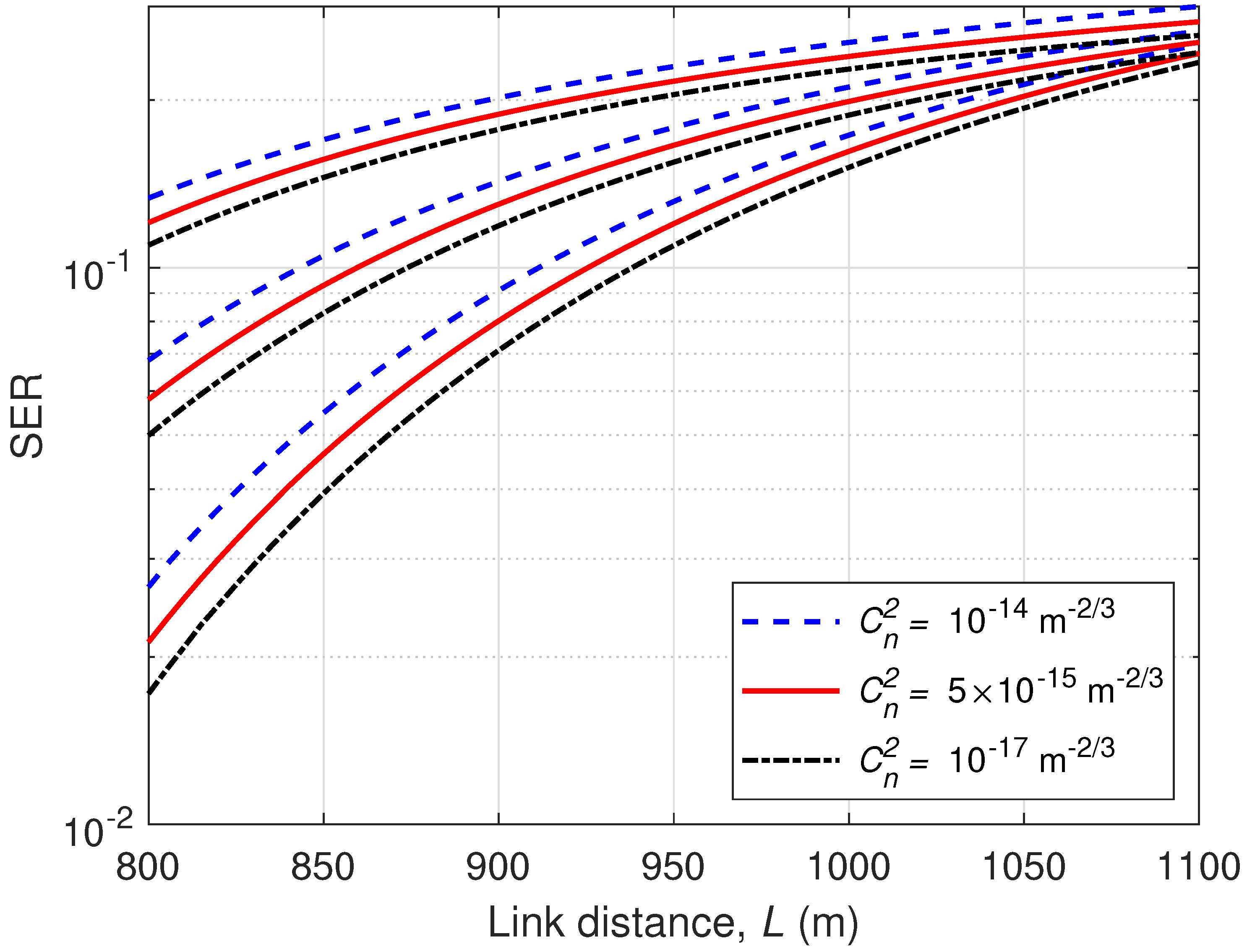
Figure 8.
SER versus SNR for different modulation schemes with/without pointing errors.


Table 1.
UAV/FSO system parameters and constants.
| Description | Parameter | Value Setting |
|---|---|---|
| UAV and FSO Tx parameters | ||
| Operational wavelength | 1.55 | |
| Beam waist radius of Tx | 0.3–0.08 m | |
| The modulation index | m | 1 |
| In-phase, quadrature distances | 8, 4 | |
| Transmitted power per symbol | −15 ÷ 5 dBm | |
| Variance of position deviation | 30 cm | |
| Variance of orientation deviation | 6 cm | |
| FSO link parameters | ||
| Link length | L | 800 m ÷ 900 m |
| Attenuation coefficient | 3.436 | |
| Strength of weak turbulence | m | |
| Strength of moderate turbulence | m | |
| Strength of strong turbulence | m | |
| FSO Rx parameters | ||
| Lens radius | r | 0.04 m |
| Average APD gain | G | 18 ÷ 30 |
| Excess noise factor of APD | F | 2.75 |
| Electrical bandwidth of APD | Hz | |
| Optical filter bandwidth | m | |
| The Planck constant | m Kg/s | |
| APD’s load resistance | 1000 | |
| Receiver noise temperature | T | 3000 K |
| Ionization factor | 0.7 | |
| Boltzmann’s constant | J/K | |
| Amplifier noise figure | 2 | |
| Receiver aperture diameter | D | 0.08 m |
| Rx’s FOV angle | 20 mrad | |
| Variance of position deviation | 30 cm | |
| Variance of orientation deviation | 6 cm | |
| Spectral radiance of the background radiations | Watts/cm2-μm-srad |
Publisher’s Note: MDPI stays neutral with regard to jurisdictional claims in published maps and institutional affiliations. |
© 2021 by the author. Licensee MDPI, Basel, Switzerland. This article is an open access article distributed under the terms and conditions of the Creative Commons Attribution (CC BY) license (https://creativecommons.org/licenses/by/4.0/).
Share and Cite
MDPI and ACS Style
Trung, H.D. Performance of UAV-to-Ground FSO Communications with APD and Pointing Errors. Appl. Syst. Innov. 2021, 4, 65. https://doi.org/10.3390/asi4030065
AMA Style
Trung HD. Performance of UAV-to-Ground FSO Communications with APD and Pointing Errors. Applied System Innovation. 2021; 4(3):65. https://doi.org/10.3390/asi4030065
Chicago/Turabian StyleTrung, Ha Duyen. 2021. "Performance of UAV-to-Ground FSO Communications with APD and Pointing Errors" Applied System Innovation 4, no. 3: 65. https://doi.org/10.3390/asi4030065