Article

Stock Market Prediction Using Deep Reinforcement Learning

by
Alamir Labib Awad
*,
Saleh Mesbah Elkaffas
and
Mohammed Waleed Fakhr
College of Computing and IT, Arab Academy for Science, Technology and Maritime Transport, Alexandria 5517220, Egypt
*
Author to whom correspondence should be addressed.
Appl. Syst. Innov. 2023, 6(6), 106; https://doi.org/10.3390/asi6060106
Submission received: 5 September 2023 / Revised: 24 October 2023 / Accepted: 3 November 2023 / Published: 10 November 2023
(This article belongs to the Special Issue Advancements in Deep Learning and Its Applications)

Abstract

:
Stock value prediction and trading, a captivating and complex research domain, continues to draw heightened attention. Ensuring profitable returns in stock market investments demands precise and timely decision-making. The evolution of technology has introduced advanced predictive algorithms, reshaping investment strategies. Essential to this transformation is the profound reliance on historical data analysis, driving the automation of decisions, particularly in individual stock contexts. Recent strides in deep reinforcement learning algorithms have emerged as a focal point for researchers, offering promising avenues in stock market predictions. In contrast to prevailing models rooted in artificial neural network (ANN) and long short-term memory (LSTM) algorithms, this study introduces a pioneering approach. By integrating ANN, LSTM, and natural language processing (NLP) techniques with the deep Q network (DQN), this research crafts a novel architecture tailored specifically for stock market prediction. At its core, this innovative framework harnesses the wealth of historical stock data, with a keen focus on gold stocks. Augmented by the insightful analysis of social media data, including platforms such as S&P, Yahoo, NASDAQ, and various gold market-related channels, this study gains depth and comprehensiveness. The predictive prowess of the developed model is exemplified in its ability to forecast the opening stock value for the subsequent day, a feat validated across exhaustive datasets. Through rigorous comparative analysis against benchmark algorithms, the research spotlights the unparalleled accuracy and efficacy of the proposed combined algorithmic architecture. This study not only presents a compelling demonstration of predictive analytics but also engages in critical analysis, illuminating the intricate dynamics of the stock market. Ultimately, this research contributes valuable insights and sets new horizons in the realm of stock market predictions.

1. Introduction

Stock market investment, a cornerstone of global business, has experienced unprecedented growth, becoming a lucrative, yet complex field [1,2]. Predictive models, powered by cutting-edge technologies like artificial intelligence (AI), sentiment analysis, and machine learning algorithms, have emerged to guide investors in their decision-making processes [3,4,5]. Key among these techniques are convolutional neural networks (CNNs), recurrent neural networks (RNNs), and long short-term memory (LSTM), all rooted in neural network methodologies. These intelligent software systems assist traders and investors in augmenting their trading strategies [6]. However, existing predictive models struggle to adapt swiftly to unforeseen market events, influenced by intricate external factors such as economic trends, market dynamics, firm growth, consumer prices, and industry-specific shifts. These factors impact stock prices, leading to unpredictable outcomes [7,8]. Hence, a fundamental analysis integrating economic factors and the ability to analyze financial news and events is imperative. Historical datasets, fundamental to stock models, often contain noisy data, demanding meticulous handling for accurate predictions. The volatile nature of stock markets, characterized by rapid fluctuations, requires precise predictions [9,10]. Diverse sources of stock market data, including media, news headlines, articles, and tweets, play a crucial role. Natural language processing (NLP) algorithms, particularly sentiment analysis, enable the extraction of sentiments from social media, news feeds, or emails. Sentiments are categorized as positive, negative, or neutral through machine learning (ML) or deep learning (DL) algorithms. This research pioneers a unique approach by combining deep reinforcement learning (DRL) and sentiment analysis from the NLP paradigm, resulting in a robust cognitive decision-making system. DRL processes multidimensional and high-dimensional resource information to generate output actions based on input data without supervision, addressing complexities posed by rapid market changes, incomplete information, and various external factors. This paper presents significant contributions, including:
  • The utilization of NLP to preprocess news and media data and discern market sentiments related to stocks. Fine-tuning BERT is employed in conjunction with TF-IDF to achieve maximum accuracy.
  • Sourcing historical stock price datasets from reputable platforms such as S&P, Yahoo, NASDAQ, etc.
  • Application of variation mode decomposition (VMD) for signal decomposition, followed by LSTM implementation to predict prices.
  • Implementation of DRL, integrating NLP, historical data, and sentiment analysis from media sources to predict stock market prices for specific businesses based on agents and actions.
The subsequent sections of this paper are organized as follows. Section 1 provides a comprehensive literature review on the topic, while Section 3 discusses the necessary background. Section 4 outlines the problem statement and algorithms employed in the project. Section 5 presents the proposed architecture for stock prediction, delving into its components. The implementation and results are discussed in Section 6, and finally, Section 7 concludes the paper.

2. Related Work

Stock price prediction efforts have centered on supervised learning techniques, such as neural networks, random forests, and regression methods [11]. A detailed analysis by authors [12] underscored the dependency of supervised models on historical data, revealing constraints that often lead to inaccurate predictions. In a separate study [13], speech and deep learning (DL) techniques were applied to stock prediction using Google stock datasets from NASDAQ. The research demonstrated that employing 2D principal component analysis (PCA) with deep neural networks (DNN) outperformed the results obtained with two-directional PCA combined with radial bias function neural network (RBFNN), highlighting the efficacy of specific methodologies in enhancing accuracy. Another comprehensive survey [14] explored various DL methods, including CNN, LSTM, DNN, RNN, RL, and others, in conjunction with natural language processing (NLP) and WaveNet. Utilizing datasets sourced from foreign exchange stocks in Forex markets, the study employed metrics like mean absolute percentage error (MAPE), root mean square error (RMSE), mean square error (MSE), and the Sharpe ratio to evaluate performance. The findings highlighted the prominence of RL and DNN in stock prediction research, indicating the increasing popularity of these methods in financial modeling. While this study covered a wide array of prediction techniques, it notably emphasized the absence of results related to combining multiple DL methods for stock prediction. In a different studies [15,16], four DL models utilizing data from NYSE and NSE markets were examined: MLP, RNN, CNN, and LSTM. These models, when trained separately, identified trend patterns in stock markets, providing insights into shared dynamics between the two stock markets. Notably, the CNN-based model exhibited superior results in predicting stock prices for specific businesses. However, this study did not explore hybrid networks, leaving unexplored potential in creating combined models for stock prediction. Additionally, advances in machine learning have led to considerable progress in speech recognition, language processing, and image classification across various applications [17]. Researchers have applied digital signal processing methods to stock data, particularly focusing on time series data analysis [18]. Moreover, reinforcement learning (RL) has emerged as a method capable of overcoming the limitations of traditional supervised learning approaches. By combining financial asset price prediction with the allocation step, RL algorithms can make optimal decisions in the complex stock market environment [19]. While LSTM techniques have been extensively researched for stock prediction due to their ability to efficiently process large datasets, challenges arise from the need for substantial historical data and considerable computational resources [20]. A critical issue with LSTM models is their limited capacity to offer rational decisions to investors, such as whether to buy, sell, or retain stocks based on predictions [21]. However, a recent study [22] demonstrated the potential of combining LSTM with sentiment analysis, providing valuable support to stock investors in decision-making processes. Furthermore, researchers have explored support vector machine (SVM) techniques in time series prediction. Despite their accuracy, SVM models require extensive datasets and involve time-consuming training processes [23]. In the comprehensive review of existing literature, it became evident that both supervised and unsupervised machine learning models have limitations, despite their efficiency in predicting time series data. Researchers have identified specific challenges associated with raw data characteristics, leading to barriers to accurate stock market predictions [24,25]. To address these limitations, this paper introduces a novel approach that integrates deep reinforcement learning (DRL) and sentiment analysis. By combining these advanced techniques, the study aims to overcome the shortcomings of traditional machine learning models, enhancing the accuracy of stock price predictions while facilitating informed decision-making for investors.

3. Background

This section provides essential context for understanding the research presented in this paper.

3.1. Deep Learning

Artificial neural networks (ANNs) replicate the complex operations of the human brain, enabling tasks such as classification and regression. ANNs comprise interconnected neurons organized in layers. Traditionally limited to a few layers due to computational constraints, modern ANNs, powered by GPUs and TPUs, support numerous hidden layers, enhancing their ability to detect nonlinear patterns as shown in Figure 1. Deep learning with ANNs finds applications in diverse fields, including computer vision, health care, and predictive analysis.

3.2. Recurrent Neural Network

Recurrent neural networks (RNNs) excel in processing sequential data. They possess a memory feature, retaining information from previous steps in a sequence as shown in Figure 2. RNNs incorporate inputs (“x”), outputs (“h”), and hidden neurons (“A”). A self-loop on hidden neurons signifies input from the previous time step (“t − 1”). However, RNNs face challenges like the vanishing gradient problem, mitigated by techniques like long short-term memory (LSTM) units. For instance, if the input sequence comprises six days of stock opening price data, the network unfurls into six layers, each corresponding to the opening stock price of a single day. However, a significant challenge confronting RNNs is the vanishing gradient problem, which has been effectively addressed through various techniques, including the incorporation of long short-term memory (LSTM) units into the network.

3.3. LSTM

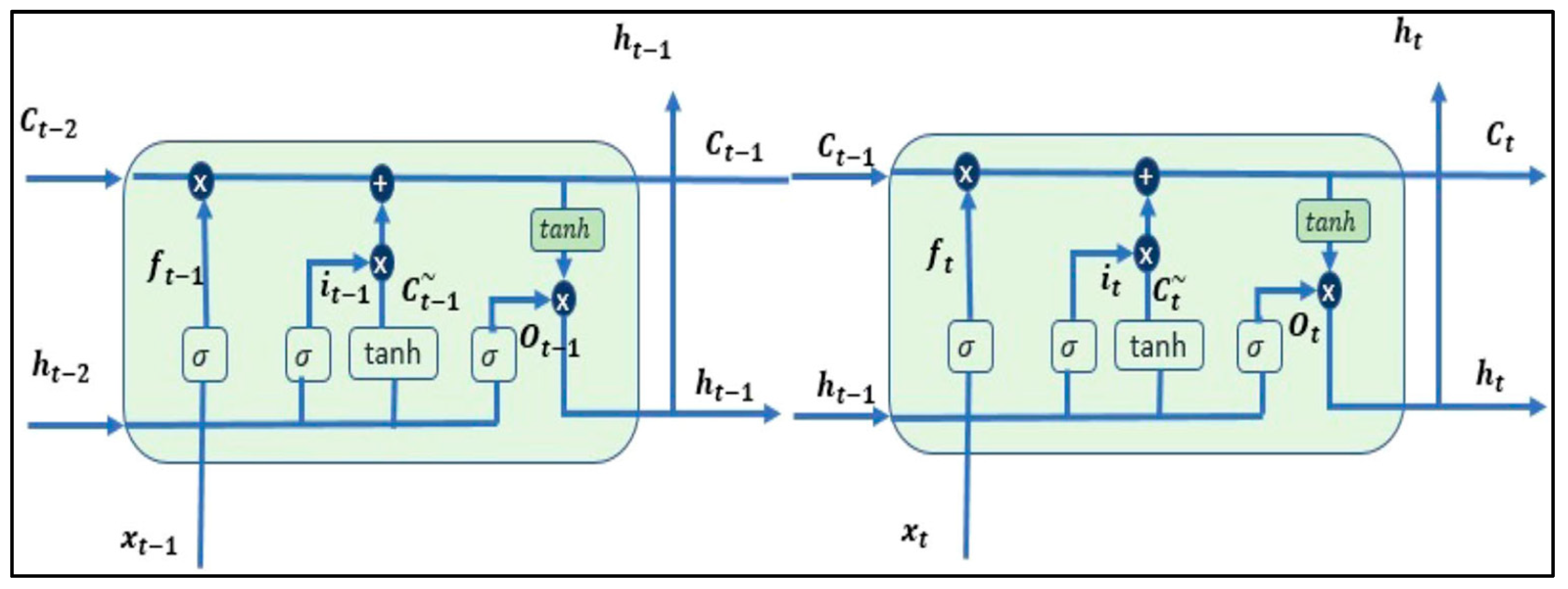
LSTM enhances RNNs’ memory, crucial for handling sequential financial data. LSTM units, integrated into RNNs, have three gates: input gate (i), forget gate (f), and output gate (o). These gates use sigmoid functions to write, delete, and read information, addressing long-term dependencies and preserving data patterns. In the LSTM architecture illustrated in Figure 3, three gates play pivotal roles:
  • Input Gate (i): This gate facilitates the addition of new information to the cell state.
  • Forget Gate (f): The forget gate selectively discards information that is no longer relevant or required by the model.
  • Output Gate (o): Responsible for choosing the information to be presented as the output.
Each of these gates operates utilizing sigmoid functions, transforming values into a range from zero to one. This mechanism empowers LSTMs to adeptly write, delete, and read information from their memory, rendering them exceptionally skilled at handling long-term dependencies and preserving crucial patterns in data. Crucially, LSTMs address the challenge of the vanishing gradient, ensuring that gradient values remain steep enough during training. This characteristic significantly reduces training times and markedly enhances accuracy, establishing LSTMs as a foundational technology in the domain of sequence prediction, especially for intricate datasets prevalent in financial markets.

3.4. Reinforcement Learning

Reinforcement learning involves an agent making decisions in different scenarios. It comprises the agent, environment, actions, rewards, and observations. Reinforcement learning faces challenges such as excessive reinforcements and high computational costs, especially for complex problems. The dynamics of reinforcement learning are encapsulated in Figure 4, illustrating the interaction between the agent and its environment. Notably, states in this framework are stochastic, meaning the agent remains unaware of the subsequent state, even when repeating the same action.
Within the realm of reinforcement learning, several crucial quantities are determined:
  • Reward: A scalar value from the environment that evaluates the preceding action. Rewards can be positive or negative, contingent upon the nature of the environment and the agent’s action.
  • Policy: This guides the agent in deciding the subsequent action based on the current state, helping the agent navigate its actions effectively.
  • Value (V): Represents the long-term return, factoring in discount rates, rather than focusing solely on short-term rewards (R).
  • Action Value: Like the reward value, but incorporates additional parameters from the current action. This metric guides the agent in optimizing its actions within the given environment.
Despite the advantages of reinforcement learning over supervised learning models, it does come with certain drawbacks. These challenges include issues related to excessive reinforcements, which can lead to erroneous outcomes. Additionally, reinforcement learning methods are primarily employed for solving intricate problems, requiring substantial volumes of data and significant computational resources. The maintenance costs associated with this approach are also notably high.
This study focuses on predicting gold prices based on next-day tweets sourced from news and media datasets. Gold prices exhibit rapid fluctuations daily, necessitating a robust prediction strategy. To achieve accurate predictions, this research employs a comprehensive approach integrating deep reinforcement learning (DRL), long short-term memory (LSTM), variational mode decomposition (VMD), and natural language processing (NLP). The prediction time spans from 2012 to 2019, utilizing tweets related to gold prices. DRL is enhanced by incorporating sentiment analysis of media news feeds and Twitter data, elevating prediction accuracy. The dataset used for this analysis was retrieved from the link https://www.kaggle.com/datasets/ankurzing/sentiment-analysis-in-commodity-market-gold accessed on 1 February 2023. This dataset, spanning from 2000 to 2021, encompasses diverse news sources and is meticulously classified as positive or negative by financial experts, ensuring the robustness and reliability of the data.

3.5. Deep Reinforcement Learning

Reinforcement learning (RL) operates as a trial-and-error methodology aimed at maximizing desired outcomes. Deep reinforcement learning (DRL) combines principles of deep learning and RL, where neural networks are trained to generate values crucial for reinforcement learning, as illustrated in Figure 5. DRL leverages prior learning from the environment and applies this knowledge to new datasets, enhancing its adaptability and learning capabilities. This approach revolves around a value function, defining the actions undertaken by the agent. In the realm of RL, the state is inherently stochastic, mirroring the inherent randomness and transitions found in variables within dynamic environments like stock markets. These variables shift between states based on underlying assumptions and probabilistic rules [26,27]. The Markov decision process (MDP) serves as a fundamental framework for modeling stochastic processes involving random variables. MDPs are instrumental in describing RL problems, particularly in managing tasks within rapidly changing environments [28]. Within the RL framework, the agent, functioning as a learner or decision-maker, interacts with the environment. In the context of MDP, the interactions between the agent and the environment define the learning process. At each step, denoted as t ∈ {1, 2, 3, …, T}, the agent receives information about the current state of the environment, represented as s_t ∈ S. Based on this information, the agent selects and executes an action, denoted as a_t ∈ A. Subsequently, if the agent transitions to a new state, the environment provides a reward, R_(t + 1) ∈ R, to the agent as feedback, influencing the quality of future actions. This iterative process encapsulates the essence of MDPs in RL problem-solving, forming a crucial foundation for adaptive learning strategies.
Another objective of reinforcement learning is to maximize the cumulative reward instead of the immediate reward [29]. Suppose the cumulative reward is represented by G t and immediate reward by R t :
E G t = E [ R t + 1 + R t + 2 + + R T ]
In Equation (1), the reward is received at a terminal state T. This implies Equation (1) will hold good when the problem ends in terminal state T, also known as the episodic task [30]. In problems involving continuous data, the terminal state is not available, i.e., T = ∞. A discount factor γ is introduced in Equation (2), which represents the cumulative reward, and 0 γ 1 to provide:
G t = γ 0 R t + 1 + γ 1   R t + 2 + γ 2 R t + 3 + γ k 1 T t + k +
G t = 0 γ k R t + k + 1
To perform an action in the given state by the agent, value functions in RL methods determine the estimate of actions. The agent determines the value functions based on what future actions will be taken [31]. Bellman’s equations are essential in RL, as they provide the fundamental property for value functions and solve MDPs. Bellman’s equations support the value function by calculating the sum of all possibilities of expected returns and weighing each return by its probability of occurrence in a policy [32].

3.6. Classification of the DRL Algorithms

Learning in DRL is based on actor or action learning, where policy learning is done to perform the best action at each state. The policy is obtained from data, and this learning continues with actions based on the learned policy. The agent will be trained in reinforcement learning based on critic-only, actor-only, and critic–actor approaches. RL algorithms are classified based on these three approaches [33].
In the critic-only approach, the algorithm will learn to estimate the value function by using a method known as generalized policy iteration (GPI). GPI involves the steps of policy evaluation, i.e., determining how good a given policy is and the next step of policy improvement. Here, the policy is improved by selecting greedy actions in relation to value functions obtained from the evaluation step. In this manner, the optimal policy is achieved [34].
The actor-only approach estimates the gradient of the objective by maximizing rewards with respect to the policy parameters based on an estimate. The actor-only approach is also known as the policy gradient method. Here, the policy function parameter will take the state and action as input to return the probability of the action in the state [35]. Suppose θ is the policy parameter, Gt is the expected reward at time t, and the estimate for maximizing rewards is given in Equation (3), where π represents the policy and at and st represent the action and state, respectively, at time t.
θ t + 1 = θ t + α l n π a t s t , θ t G t
The actor–critic approach will form the policy as the actor will select actions, and the critic will evaluate the chosen actions. Hence, in this approach, the policy parameters θ will be adjusted for the actor to maximize the reward predicted by the critic. Here, the value function estimate for the current state is summed as a baseline to accelerate learning. The policy parameter θ of the actor is adjusted to maximize the total future reward. Policy learning is done by maximizing the value function [36].
DRL is an action–critic-based value learning function that compromises current and future rewards [37]. The stock prediction problem can be formulated by describing the state space, action space, and reward function. Here, the state space is the environment designed to support single or multiple stock trading by considering the number of assets to trade in the market. The state space will show a linear increase with increasing assets. The state space has two components: the position state and the market signals. The position state will provide the cash balance and shares owned in each asset, and the market signals will contain all necessary market features for the asset as tuples [38]. The information is provided to the agent to make predictions of market movement. Here, the information is a hypothesis based on technical analysis and of the future behavior of the financial market based on its past trends. The information will also be used by economic and industry conditions, media, and news releases.

3.7. Natural Language Processing

Natural language processing (NLP) analyzes natural languages such as English, French, etc., and makes computer systems interpret texts like humans. The human language is complicated to understand; hence, this is an ever-evolving field with endless applications. Every sentence should pass a preprocessing phase with six steps to build any NLP model. First is the tokenization phase, in which the sentence is split into a group of words. Second, the lowercasing phase converts every word to its lowercase form. Third, the stop words do not impact the sentence’s meaning, so they are removed in this step. Fourth, every word is transformed into its root word in the steaming phase. Last, the lemmatization phase reduces the number of characters representing the word. After this preprocessing phase, there is the feature extraction in which the sentence is transformed from its textual representation into a mathematical representation called word embedding. Many word embedding approaches have been developed over the years. The classical approaches involve wrod2vec and Glove, while the modern ones include BERT.

3.8. Sentiment Analysis

Sentiment analysis aims to identify the opinion toward a product from a text. There are three modes toward a product: positive, negative, and neutral. Two main approaches are used in sentiment analysis: the supervised approach and the lexicon approach. In the supervised approach, the sentences are provided to the classification model along with their label, positive or negative. Then, the sentences are transformed into vectors, and the model makes a classification for these vectors.
On the other hand, the lexicon-based approach relies on the language dictionary itself. The model has a list of positive and negative words. The sentences are divided into words, each with a semantic score. Finally, the model calculates the total semantics of the sentence and decides whether it is a positive or negative sentence.

3.9. TFIDF

TF-IDF stands for term frequency–inverse document frequency. It is used for document search by getting a query as input and finding the relevant documents as output. It is a statistical analysis technique used to know the importance of a word inside a document. It calculates the frequency of a word inside a document, compares it with the frequency of the word inside all documents, and compares the two values. The assumption is that if the word is repeated many times in a document and rarely appears in other documents, this means that this word is vital for this document.

3.10. BERT

Bidirectional encoder representations from transformers (BERT) is based on deep learning transformers for natural language processing. BERT is trained bidirectionally, which means it analyzes the word and the surrounding words in both directions. Reading in both directions allows the model to understand the context deeply. BERT models are already pretrained, so they already know the word representation and the relationships between them. BERT is a generic model that can be fine-tuned for specific tasks like sentiment analysis tasks. BERT contains a stack of transformers, each consisting of an encoder and decoder network. It has two versions, the base version and the large one, which gives the best results compared to any other model.

4. Problem Statement

In the complex landscape of stock markets, the central objective of trading resides in the precise forecasting of stock prices. This accuracy is paramount, as it directly influences investors’ confidence, shaping their decisions on whether to buy, hold, or sell stocks amid the inherent risks of the market. Extensive scholarly research emphasizes the critical necessity for efficiency in addressing the challenges associated with stock price prediction. Efficient predictions are not just advantageous but pivotal, empowering investors with the knowledge needed for astute decision-making. Market efficiency, a foundational concept in this domain, refers to the phenomenon where stock prices authentically mirror the information available in the current trading markets. It is essential to recognize that these price adjustments might not solely stem from new information; rather, they can be influenced by existing data, leading to outcomes that are inherently unpredictable. In this context, our research endeavors to enhance the precision of stock price predictions, addressing the need for informed and confident decision-making among investors.

5. Proposed Novel Architecture for Stock Market Prediction

This research is developed to predict stock prices by utilizing the DRL model, NLP, and the variational mode decomposition plus RNN. The model receives stock historical data and news data and generates the final trading decision (buy or sell) to achieve the maximum profit. The architecture is provided in Figure 6. The architecture is developed using three phases: the NLP phase, the VMD plus RNN phase, and the DRL phase.
In order to facilitate the implementation of the proposed framework the code is divided into three major modules that can be summarized in Algorithm 1.
Algorithm 1: Stock Price prediction framework
Data: Raw news data, historical stock dataset
Result: Final trading decision (buy, sell)
NLP Module:
           Input: Raw news data
           Output: classified sentences to positive or negative
                     Preprocessing:
                                   Read the raw news dataset.
                                   Tokenize the sentences.
                                   Convert words to lowercase.
                                   Remove stop words.
                                   Stem the sentences.
                                   Lemmatize the words.
                     Feature extraction using BERT and TFIDF
                                   Utilize BERT and TFIDF to extract features from news data.
                     Sentence classification as positive or negative
Prediction Module:
           Input: Historical stock data
           Output: Predicted stock prices
           Steps:
                     Read stock data signal.
                     Signal decomposition using variational mode decomposition.
                     Apply decomposed signal to the LSTM.
                     Predict stock prices for the next days based on decomposed signal by LSTM.
Decision-Making Module:
           Input: Output from NLP Module, output from prediction module
           Output: Final decision (buy/sell)
           Steps:
                                   Combine sentiment analysis results with the predicted prices.
                                   Train deep Q learning network to make trading decisions.
                                   Implement DQN.
Results
                                   Generate the suitable decision—sell or buy.

5.1. Sentiment Analysis Phase

NLP will determine general sentiments from news releases or social media to integrate with state representation. Sentiment analysis is considered for better prediction because media and news influence stock movements. Sentiment analysis uses the models, namely, the multinomial classification model and BERT classifier, to evaluate the accuracy of sentiment prediction. More than one model can be applied by combining them to improve prediction accuracy. Here, NLP will demystify text data to solve the language problem. The approach is used to identify unexplored weaknesses in the model and to understand if media will play a role in predicting stock prices [39].
In sentiment analysis, the neural classifier TF-IDF (term frequency–inverse document frequency) is used. This algorithm will use the frequency of words in the news or media datasets to determine how the words are relevant in each dataset related to a particular stock. TF-IDF in sentiment analysis is popular, as it assigns a value to a term according to its importance in the text dataset or document [40]. The naturally occurring words are mathematically eliminated, and the more descriptive words in the text are selected. The other method, principal component analysis (PCA) and singular value decomposition (SVD), is used to reduce dimensionality in the dataset.
In addition to the above techniques, BERT (bidirectional encoder representation from transformer) is a DL model where the output of each element is connected to every input, and the weights are dynamically calculated with respect to their connection. Usually, language models read text from left to right or right to left, but BERT can simultaneously read text from both directions for its bidirectional characteristic. Due to its capabilities, BERT is used in NLP tasks for predicting the next sentence [41]. In NLP, mixed models tend to provide the best results from BERT. For instance, TFIDF, SVM, and BERT will provide better sentiment output from the dataset. The sentiments are further classified into four categories: extremely positive, positive, negative, and extremely negative. NLP will support investors in classifying if the news is positive or negative to decide whether to sell, buy, or hold stock.
In this phase, news data are fed to the natural language processing module to decide whether the news is positive or negative. The BERT model is used along with TFIDF in this task to achieve the most accurate results. Fine-tuning BERT is achieved by applying a binary classifier on top of BERT. This NLP phase involves the stages of preprocessing, modeling, and prediction.
  • Preprocessing: In this phase, the news dataset obtained from media or tweets is preprocessed. The preprocessing involves reading the dataset, tokenizing the sentences, converting words to lowercase, removing stop words, sentences stemmed, and finally, the words with the same meaning are grouped or lemmatized.
  • Modeling: This step involves feature extraction for the model and sentiment analysis. Sentiment analysis will first convert the tokens to the dictionary, and the dataset will be split for training and testing the model. The model is built using an artificial neural network classifier.
  • Prediction: This step will receive the testing news data and predict if the sentiment is positive or negative. This result is concatenated with the historical dataset.

5.2. Price Prediction Phase

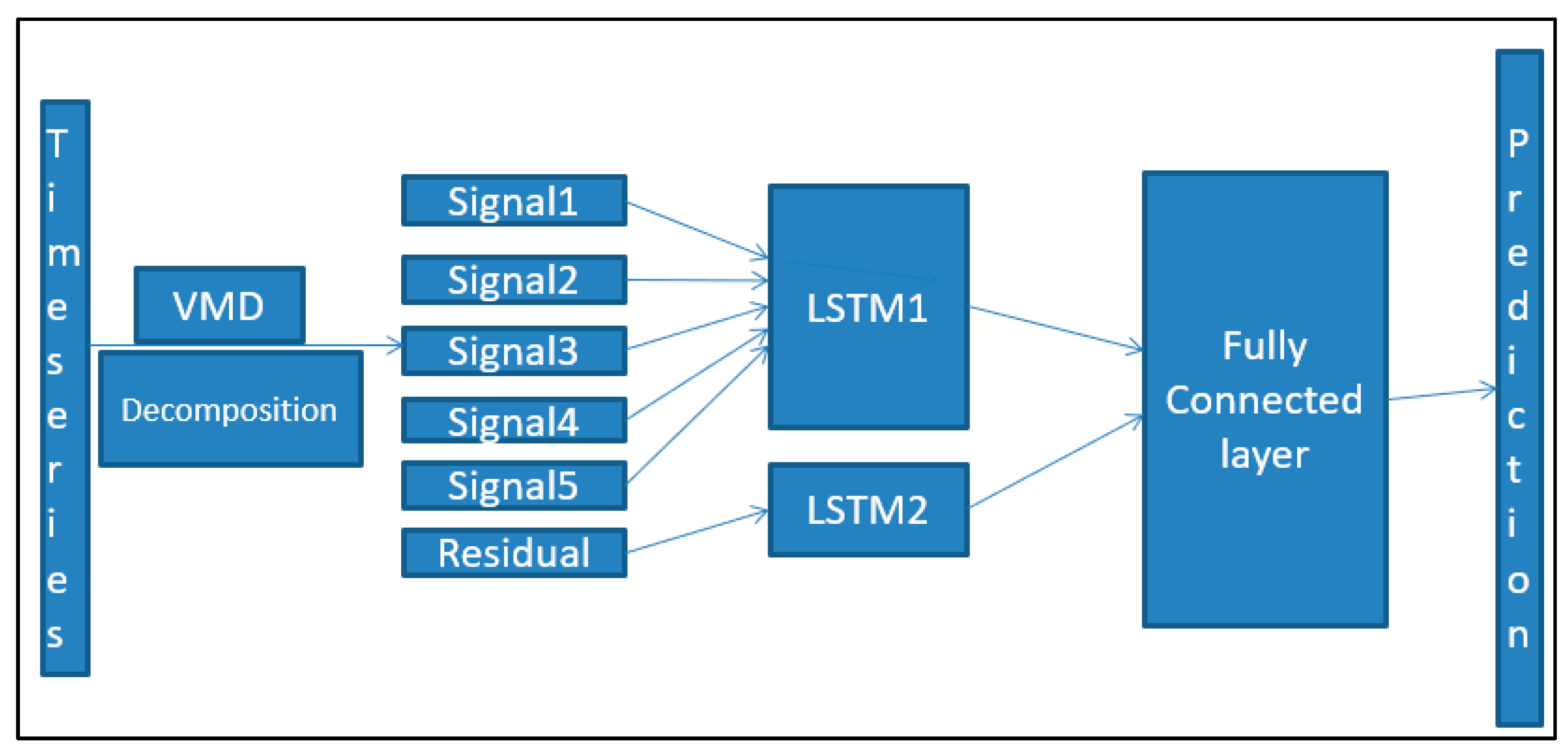
In this crucial phase, historical data are meticulously gathered and utilized to generate accurate price predictions. Recognizing the inherent complexity of stock price data, our approach employs long short-term memory (LSTM) due to its efficacy in handling temporal dependencies within time series data. Stock prices often exhibit noise, making direct analysis challenging. To mitigate this challenge, the raw signal undergoes a preprocessing step using variational mode decomposition (VMD) before being fed into the LSTM network as illustrated in Figure 7. VMD plays a pivotal role in enhancing the quality of our predictions. Its unique ability lies in effectively handling noisy data and isolating essential features. Unlike other methods, VMD excels in feature selection, making it robust against noise interference. By identifying the intricate relationship between the asset and market sentiment, VMD provides a solid foundation for our analysis. The architecture leverages the VMD component to address the complexities of real-world signals, which often comprise multiple frequency components. VMD achieves this by employing distinct filters to separate these components. The filtering process, based on intrinsic mode functions (IMFs), proves instrumental in denoising the signals, ensuring that the subsequent time series data are clear and reliable. During the VMD phase, the input signal is intelligently divided into five sub-signals. Each of these sub-signals undergoes meticulous analysis, enabling the generation of precise predictions using the LSTM model. The resulting predicted prices, derived from these sub-signals, are subsequently fed into our deep reinforcement learning (DRL) model, forming a critical link in our comprehensive analysis. It is imperative to note that the VMD phase is executed using the “vmdpy” library in Python, ensuring a robust and efficient preprocessing step in our price prediction methodology. This meticulous approach enhances the accuracy and reliability of our predictions, laying a solid foundation for our subsequent analyses.

5.3. The Deep Reinforcement Learning Phase

The last phase is the DRL model, from which the final decision is generated. The input to this phase is the output from the sentiment analysis module, the predicted prices from the LSTM, and some technical indicators. The DRL used in this phase is deep Q learning with a reply buffer. The neural network is trained to generate the Q values for all the possible actions based on the current environment state, which is fed to the neural network as input.
Therefore, the proposed architecture and algorithm depend on historical and media or news datasets. The architecture consists of three phases: NLP, prediction, and DRL. The combined algorithm of sentiment and analysis and DRL are used to obtain predictions for stock.

6. Implementation and Discussion of Results

The implementation of our framework is carried out utilizing cloud GPUs, leveraging the advantages of cloud computing for enhanced processing capabilities. Rigorous evaluation and fine-tuning of each code module are conducted to ensure optimal accuracy at every phase. The efficiency of the proposed framework is comprehensively evaluated and compared with benchmark trading strategies to validate its effectiveness.

6.1. Sentiment Analysis Phase

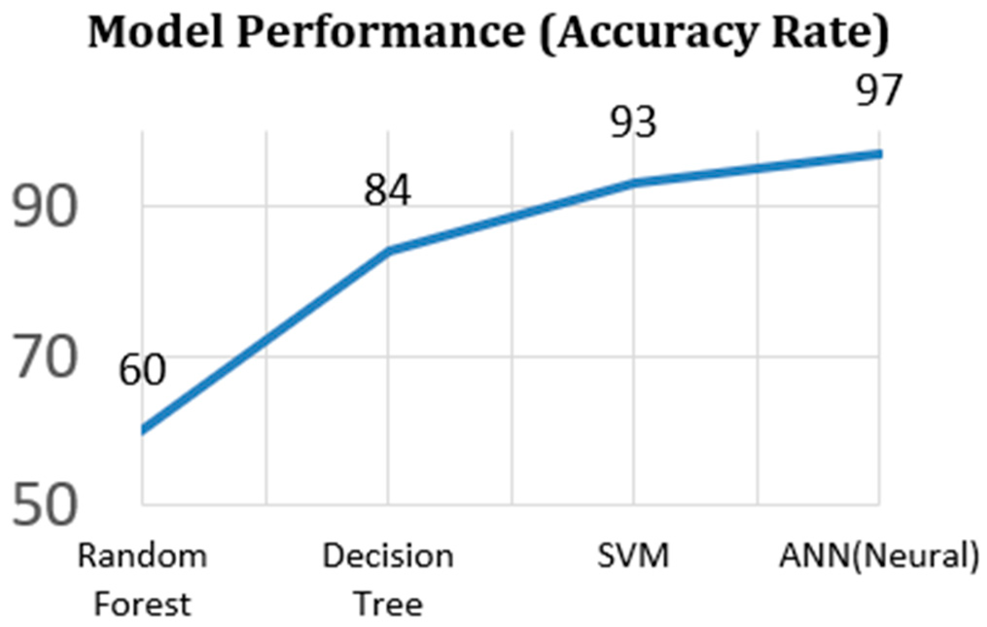
In the sentiment analysis phase, various classification algorithms coupled with different preprocessing models are tested to determine the most accurate algorithm. The results, as shown in Table 1, underscore the superiority of the combination of TFIDF and BERT, which yielded a remarkable accuracy of 96.8%. Extensive analytics, including classification techniques and model overfitting identification, were performed. Visualization, especially using artificial neural networks (ANN) with BERT and TFIDF, played a crucial role in comprehending the training-prediction dynamics. The ANN model exhibited exceptional performance, boasting an accuracy rate of 97%, as depicted in Figure 8.
Table 1 and Figure 8 show that BERT with TFIDF and ANN provided better accuracy than the other combinations. The BERT model is a robust predictor without bias, given these predicted outputs and determined values. BERT provided performance based on sensitivity to the length of sentences, number of words, and opposite statements.
The robustness of the BERT model, free from biases, is evidenced by its performance, which was influenced by various factors such as sentence length, word count, and contradictory statements.

6.2. Stock Prices Prediction Phase

The next phase is the price prediction phase, and this is done by decomposing the signal into five sub-signals and passing the output to the LSTM to make the prediction. The decomposing step is implemented using Python’s “vmdpy” library with the hyperparameters in Table 2.
The price prediction is conducted via a recurrent neural network (LSTM) with the configurations defined in Table 3.
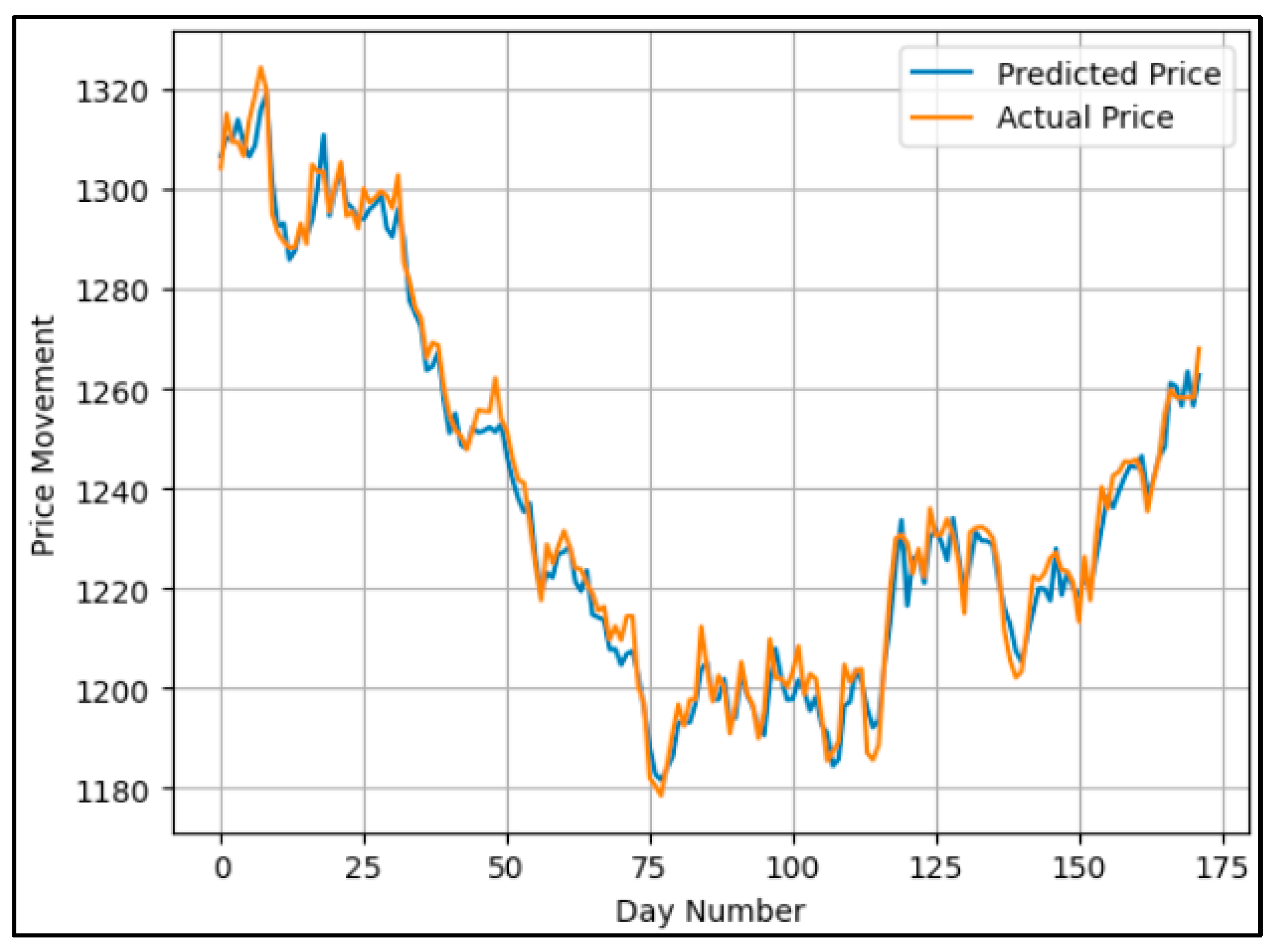
It is important to note that the accurate prediction from this phase leads to accurate decisions from the DRL phase. The efficiency of this prediction is evaluated, and the results are shown in Figure 9, comparing the actual and predicted prices. The figure shows that our prediction module works very well, as there is a significant correlation between the actual and the predicted prices.

6.3. Final Decision Phase

The next phase is the deep reinforcement learning phase, which will make the final decision. The implementation relies on the famous architecture of deep Q learning, which belongs to the value-based category of DRL algorithms. Table 4 shows the configuration for the implemented network. The DQN relies on a reply buffer with two deep neural networks: one is the main network, and the other is the target network. Both networks have the same architecture with three layers.
The final decision phase employs deep reinforcement learning (DRL), specifically the deep Q learning architecture, a value-based DRL algorithm. The implementation details are provided in Table 4. The state representation includes factors like historical and predicted prices, sentiment analysis outputs, and technical indicators like relative strength index (RSI) and momentum (MOM). The action space consists of four actions: buy, buy more, sell, and sell more.
The efficiency of the entire framework is deeply rooted in the accurate predictions from the stock price prediction phase. The DRL model’s capability to make informed decisions based on these predictions is crucial for successful trading strategies.

6.4. Algorithms in Comparison

The gold dataset was processed using the algorithms, namely, best stock benchmark, buy-and-hold benchmark, and “constantly rebalanced portfolios” (CRPs). The algorithms provided results that were compared with the proposed architecture. The metrics and values determined using these algorithms are provided in Table 5. The values obtained are rounded to the nearest whole number. The classical buy-and-hold benchmark is quite simple, where the user buys gold with all his money at the beginning of the period and waits till the end of the period, then sells all his gold, and the total profit is the difference between his wealth at the start and end of the period.

6.5. Evaluation Metrics

  • Accumulated wealth rate
Accumulated wealth rate (AWR) is a strategy in which the investor buys as much as stock based on the first-day price. Every day, calculate the total stock value based on the current price by multiplying the number of shares by the current price, then add it to the cash to get the investor’s total wealth on that day. Finally, calculate the profit or loss achieved and divide it by the total cash available at the start of the trading period. The following equation describes how the AWR can be calculated.
A W R T = t = 1 T P t   o r   L t C a s h t = 0
  • Average Max drawdown
As an intermediate step, the max drawdown (MDD) is calculated, and then the average is calculated on top of it. MMD compares the current wealth with the peak wealth to determine the maximum loss during the trading period. Consequently, the average max drawdown is the average value for the MDD during the trading period.
M D D t = P e a k   W e a l t h W e a l t h t P e a k   W e a l t h
A M D D T = t = 1 T ( M D D t )   T  
  • Calmar ratio
This calculates the mean value for the accumulated wealth rate with respect to the max of the max drawdown value. The following equation can calculate it.
A M D D T = t = 1 T ( M D D t )   T  
  • Average profit return
The profit return calculates the difference between the current and previous prices and normalizes the result to the previous price. The average profit return is the average of the previous value within the trading period, as shown in Equations (9) and (10).
P R T = t = 1 T ( P r i c e t P r i c e t 1 ) P r i c e t 1
A P R T = A v g ( P R T )
  • Average Sharpe ratio
The Sharpe ratio is defined as the meaning of the accumulated wealth rate divided by the standard deviation of the accumulated wealth rate. Moreover, the average Sharpe ratio is the average of this value during the trading period.
S R T = m e a n ( A W R T ) S t d ( A W R T )
A S R T = t = 1 T ( S R t )   T  
  • Annualized Return Rate and Annualized Sharpe Ratio
The annualized terms mean calculating the values with respect to a full year.
They are calculated with the same equations, but the trading periods will be 365.

6.6. Technical Indicators

It is important to note that our framework also considers some technical indicators like the RSI and MOM.
  • Relative Strength Index (RSI)
It is a technical momentum indicator that compares the magnitude of recent gains to recent losses in a trial to see an asset’s overbought and oversold conditions. It is calculated using the subsequent formula:
R S I = 100 100 ( 1 + R S )
where RS = average of x days’ up closes/average of x days’ down closes.
  • Momentum
Momentum is the difference between the current and last prices in the last n days. As such, it reflects the price changes speed in the stock market.

6.7. Reward Calculation

Giving the negative reward, extra weight is better to force the agent to avoid the negative rewards. The reward is calculated since the action led to profit or loss; if the action led to profit, the value of the reward would be equal to the profit. On the other hand, if the action leads to loss, the value of the reward will be three times the value of the loss that occurred. Finally, the total reward for the episode is the summation of all the rewards achieved during the episode.
R e w a r d =       P r o f i t                                                      i n   c a s e   o f   p r o f i t   3 × L o s s                                                   i n   c a s e   o f   l o s s  

6.8. State Representation

The state represents a significant element in DRL. State, in this case, consists of different components. Several experiments are conducted with different combinations of components to achieve the best state for our problem. The final state in our proposed framework consists of several elements: first, the RSI technical indicator for the last nine days; second, the MOM technical indicator for the last nine days; third, the simple moving average for the last nine days; Fourth, the simple moving average for the last two days; fifth, the predicted prices for the upcoming five days are predicted from the VMD plus LSTM; and sixth, the sentiment analysis module generates the sentiment for the current day.

6.9. Proposed Framework Results Comparison

The results from the proposed framework are compared with the benchmark trading strategies mentioned above. The results showed that the proposed framework outperformed the other algorithms in different evaluation criteria, as shown in Table 5.
The values for performance metrics are obtained from the same gold dataset earlier. The DQN results were compared with the other algorithms. The graphs were obtained to show the performance of the algorithms. The annualized wealth rate algorithm provided the following graph for metrics shown in Figure 10.
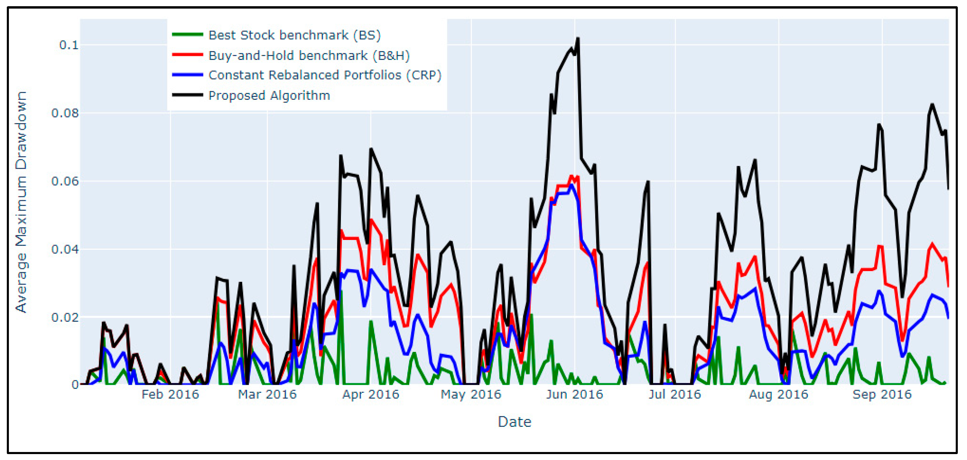
The graph for the average maximum drawdown algorithm for the performance metrics is provided in Figure 11.
In Figure 10, the peaks indicate the amount of profit possible at a certain point in time. The graphs show that regarding the annualized wealth rate, the proposed algorithm outperforms the other algorithms, and hence is effective in predicting stock value. Likewise, in Figure 11, the peaks of the proposed algorithm indicate that the results outperform other baseline algorithms. In addition, the NLP processing and the combined RNN, DQN, and VMD architecture provide better prediction results.

6.10. Ablation Study

In any AI algorithm that consists of several phases, it is essential to know the effect of each phase on the overall performance of the algorithm, so the following two subsections contain an ablation study to emphasize the effect of each module on the overall framework efficiency.

6.10.1. Effect of Using the VMD on the Price Prediction Phase

Table 6 emphasizes that utilizing the VMD layer improved performance, which reached 80% improvement in some cases. This improvement is achieved because VMD can remove the noisy data and extract the hidden important signals from the original signal.

6.10.2. Effect of Using Sentiment Analysis Module on the Framework Performance

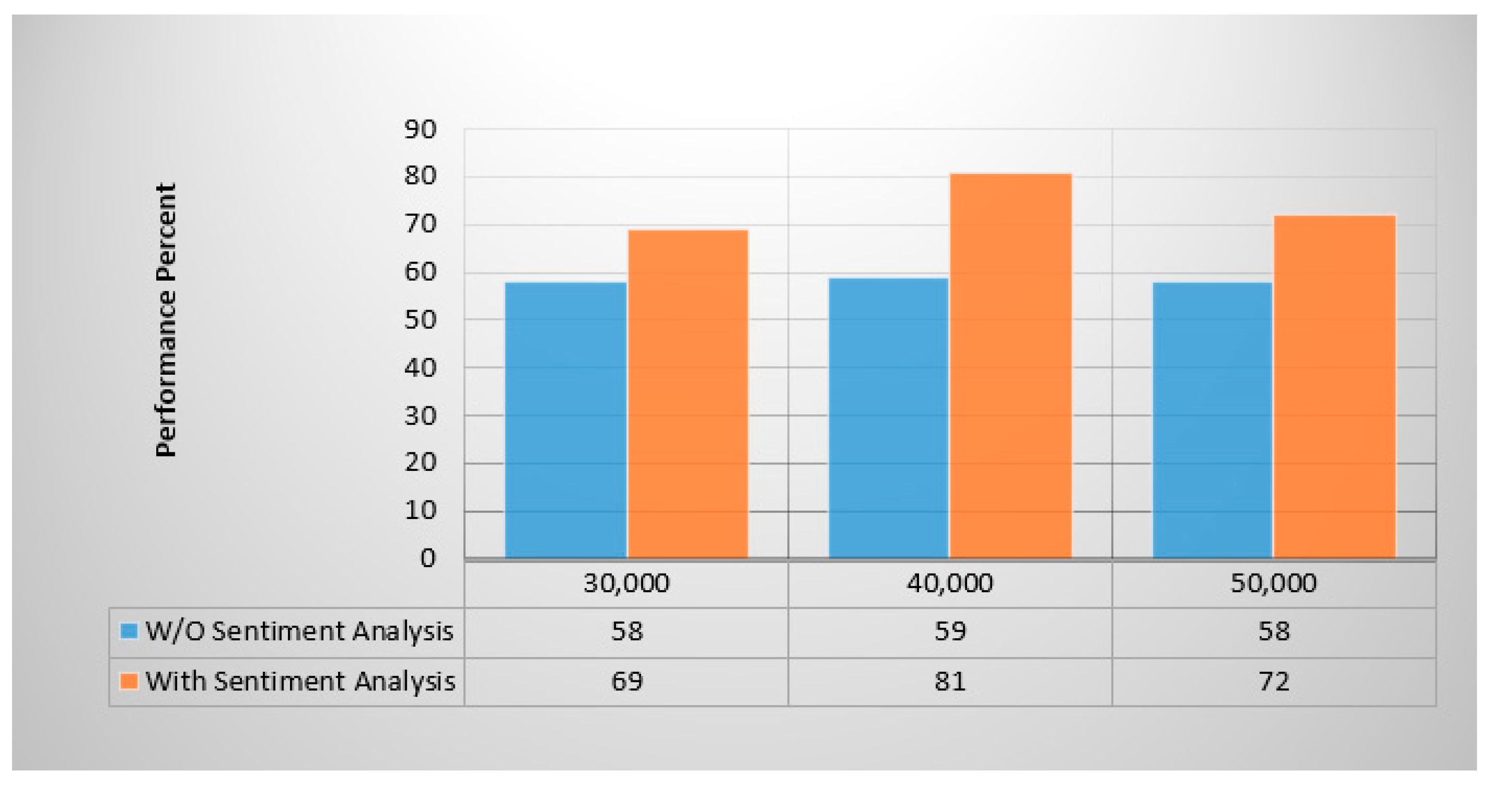
In the same context, other experiments are conducted to emphasize the efficiency of using sentiment analysis in our proposed algorithm. Figure 12 shows the performance improvement achieved by adding the sentiment analysis module to our algorithm. The experiments are done for different numbers of episodes. Each number of episodes is done at least 10 times, and the average is taken. In these experiments, the performance is measured as follows. The current day’s closing price is compared with the previous day’s closing price. If there is a price increase and the algorithm decides to sell, this is considered the correct action. On the other hand, if the algorithm decides to buy, this is considered a wrong action. The performance here is calculated as the percentage of the correct actions relative to the algorithm’s total number of actions.

7. Conclusions

This research introduces a novel architecture that combines various prediction algorithms to tackle the challenges of stock value prediction with exceptional accuracy. Specifically focusing on gold datasets, the study aimed to forecast gold prices for investors. The input data encompassed gold datasets from reputable sources such as S&P, Yahoo, and NASDAQ, representing standard stock market data. The predictive framework employed natural language processing (NLP) to process sentiments extracted from social media feeds, long short-term memory (LSTM) networks to analyze historical data, variation mode decomposition (VMD) for feature selection, and artificial neural networks (ANNs) to make predictions. Additionally, the research integrated deep reinforcement learning (DRL) algorithms and deep Q networks (DQNs) to blend sentiments with other algorithms, enabling the prediction of the opening stock value for the next day based on the previous day’s data. The processes developed for training and testing data were meticulously presented, forming the foundation of the prediction model. Comparative analysis was conducted with benchmark performance metrics, including the best stock benchmark, buy-and-hold benchmark, constant rebalanced portfolios, and DQN. Through rigorous evaluation, the proposed architecture demonstrated superior accuracy in performance metrics. Graphical representations were employed to showcase peaks indicating high values at specific times or on specific days, aligning with benchmark standards. The comparison clearly highlighted that the DQN outperformed existing algorithms, underscoring the potential of the proposed architecture to predict stocks with unparalleled precision.
Future research, which could extend this research into real-time applications within dynamic environments, such as livestock markets, holds immense promise. Such applications could provide invaluable insights into the model’s effectiveness and adaptability across different market scenarios. Moreover, the framework’s generic nature, as demonstrated in this study, suggests its versatility for application across diverse products beyond gold. This versatility transforms the model into a powerful tool for traders and investors in various sectors. Subsequent studies focusing on real-time livestock market data not only stand to validate the framework’s effectiveness but also pave the way for tailored adaptations customized to specific industries and the unique intricacies of each market.
The proposed framework contains three main modules. Each module can be enhanced with different techniques. In the sentiment analysis module, the proposed framework used classification techniques to judge whether the sentence is positive or negative. However, another primary technique that can be used is the lexicon-based technique in which the language dictionary is used to make the sentiment analysis.
In the price prediction module, the proposed framework considered the stock historical prices as a signal and used VMD as a signal-processing technique to decompose the signal into sub-signals and remove the signal noise. Several other signal-processing techniques can be used for noise removal. This area is open to research, and other signal-processing techniques may easily enhance this module if they exist.
Finally, the decision-making is undertaken by the deep reinforcement network. Several DRL techniques can be utilized in this module, giving better or worse results than the implemented one.

Author Contributions

Methodology, A.L.A., S.M.E. and M.W.F.; Software, A.L.A.; Supervision, S.M.E. and M.W.F. All authors have read and agreed to the published version of the manuscript.

Funding

This research received no external funding.

Data Availability Statement

Publicly available datasets were analyzed in this study. This data can be found here: https://www.kaggle.com/datasets/ankurzing/sentiment-analysis-in-commodity-market-gold (accessed on 1 February 2023).

Conflicts of Interest

The authors declare no conflict of interest.

References

  1. Idrees, S.M.; Alam, M.A.; Agarwal, P. A Prediction Approach for Stock Market Volatility Based on Time Series Data. IEEE Accesss 2019, 7, 17287–17298. [Google Scholar] [CrossRef]
  2. Bouteska, A.; Regaieg, B. Loss aversion, the overconfidence of investors and their impact on market performance evidence from the US stock markets. J. Econ. Financ. Adm. Sci. 2020, 25, 451–478. [Google Scholar] [CrossRef]
  3. Feng, F.; He, X.; Wang, X.; Luo, C.; Liu, Y.; Chua, T.S. Temporal Relational Ranking for Stock Prediction|ACM Transactions on Information Systems. ACM Trans. Inf. Syst. (TOIS) 2019, 37, 1–30. [Google Scholar] [CrossRef]
  4. Dirman, A. Financial distress: The impacts of profitability, liquidity, leverage, firm size, and free cash flow. Int. J. Bus. Econ. Law 2020, 22, 17–25. [Google Scholar]
  5. Ghimire, A.; Thapa, S.; Jha, A.K.; Adhikari, S.; Kumar, A. Accelerating Business Growth with Big Data and Artificial Intelligence. In Proceedings of the 2020 Fourth International Conference on I-SMAC (IoT in Social, Mobile, Analytics and Cloud) (I-SMAC), Palladam, India, 7–9 October 2020. [Google Scholar] [CrossRef]
  6. Kurani, A.; Doshi, P.; Vakharia, A.; Shah, M. A Comprehensive Comparative Study of Artificial Neural Networks (ANN) and Support Vector Machines (SVM) on Stock Forecasting. Ann. Data Sci. 2021, 10, 183–208. [Google Scholar] [CrossRef]
  7. Beg, M.O.; Awan, M.N.; Ali, S.S. Algorithmic Machine Learning for Prediction of Stock Prices. In FinTech as a Disruptive Technology for Financial Institutions; IGI Global: Hershey, PA, USA, 2019; pp. 142–169. [Google Scholar] [CrossRef]
  8. Shah, D.; Isah, H.; Zulkernine, F. Stock Market Analysis: A Review and Taxonomy of Prediction Techniques. Int. J. Financ. Stud. 2019, 7, 26. [Google Scholar] [CrossRef]
  9. Yadav, A.; Chakraborty, A. Investor Sentiment and Stock Market Returns Evidence from the Indian Market. Purushartha-J. Manag. Ethics Spiritual. 2022, 15, 79–93. [Google Scholar] [CrossRef]
  10. Chauhan, L.; Alberg, J.; Lipton, Z. Uncertainty-Aware Lookahead Factor Models for Quantitative Investing. In Proceedings of the 37th International Conference on Machine Learning (PMLR), Virtual, 13–18 July 2020; Volume 119, pp. 1489–1499. [Google Scholar]
  11. Nti, I.K.; Adekoya, A.F.; Weyori, B.A. A novel multi-source information-fusion predictive framework based on deep neural networks for accuracy enhancement in stock market prediction. J. Big Data 2021, 8, 17. [Google Scholar] [CrossRef]
  12. Sakhare, N.N.; Imambi, S.S. Performance analysis of regression-based machine learning techniques for prediction of stock market movement. Int. J. Recent Technol. Eng. 2019, 7, 655–662. [Google Scholar]
  13. Singh, R.; Srivastava, S. Stock prediction using deep learning. Multimed. Tools Appl. 2016, 76, 18569–18584. [Google Scholar] [CrossRef]
  14. Hu, Z.; Zhao, Y.; Khushi, M. A Survey of Forex and Stock Price Prediction Using Deep Learning. Appl. Syst. Innov. 2021, 4, 9. [Google Scholar] [CrossRef]
  15. Hiransha, M.; Gopalakrishnan, E.A.; Menon, V.K.; Soman, K.P. NSE Stock Market Prediction Using Deep-Learning Models. Procedia Comput. Sci. 2018, 132, 1351–1362. [Google Scholar] [CrossRef]
  16. Patel, R.; Choudhary, V.; Saxena, D.; Singh, A.K. Review of Stock Prediction using machine learning techniques. In Proceedings of the 5th International Conference on Trends in Electronics and Informatics (ICOEI), Tirunelveli, India, 3–5 June 2021; pp. 840–847. [Google Scholar]
  17. Kamath, U.; Liu, J.; Whitaker, J. Deep Learning for NLP and Speech Recognition; Springer: Cham, Switzerland, 2019; pp. 575–613. [Google Scholar]
  18. Manolakis, D.; Bosowski, N.; Ingle, V.K. Count Time-Series Analysis: A Signal Processing Perspective. IEEE Signal Process. Mag. 2019, 36, 64–81. [Google Scholar] [CrossRef]
  19. Kabbani, T.; Duman, E. Deep Reinforcement Learning Approach for Trading Automation in the Stock Market. IEEE Access 2022, 10, 93564–93574. [Google Scholar] [CrossRef]
  20. Moghar, A.; Hamiche, M. Stock Market Prediction Using LSTM Recurrent Neural Network. Procedia Comput. Sci. 2020, 170, 1168–1173. [Google Scholar] [CrossRef]
  21. Ren, Y.; Liao, F.; Gong, Y. Impact of News on the Trend of Stock Price Change: An Analysis based on the Deep Bidirectional LSTM Model. Procedia Comput. Sci. 2020, 174, 128–140. [Google Scholar] [CrossRef]
  22. Jin, Z.; Yang, Y.; Liu, Y. Stock closing price prediction based on sentiment analysis and LSTM. Neural Comput. Appl. 2019, 32, 9713–9729. [Google Scholar] [CrossRef]
  23. Parray, I.R.; Khurana, S.S.; Kumar, M.; Altalbe, A.A. Time series data analysis of stock price movement using machine learning techniques. Soft Comput. 2020, 24, 16509–16517. [Google Scholar] [CrossRef]
  24. Duan, G.; Lin, M.; Wang, H.; Xu, Z. Deep Neural Networks for Stock Price Prediction. In Proceedings of the 14th International Conference on Computer Research and Development (ICCRD), Shenzhen, China, 7–9 January 2022. [Google Scholar] [CrossRef]
  25. Huang, J.; Liu, J. Using social media mining technology to improve stock price forecast accuracy. J. Forecast. 2019, 39, 104–116. [Google Scholar] [CrossRef]
  26. Iqbal, S.; Sha, F. Actor-Attention-Critic for Multi-Agent Reinforcement Learning. In Proceedings of the 36th International Conference on Machine Learning, Long Beach, CA, USA, 10–15 June 2019; pp. 2961–2970. [Google Scholar]
  27. Singh, V.; Chen, S.-S.; Singhania, M.; Nanavati, B.; Kar, A.K.; Gupta, A. How are reinforcement learning and deep learning algorithms used for big data-based decision making in financial industries—A review and research agenda. Int. J. Inf. Manag. Data Insights 2022, 2, 100094. [Google Scholar] [CrossRef]
  28. Padakandla, S. A survey of reinforcement learning algorithms for dynamically varying environments. ACM Comput. Surv. (CSUR) 2021, 54, 1–25. [Google Scholar] [CrossRef]
  29. Silver, D.; Singh, S.; Precup, D.; Sutton, R.S. A reward is enough. Artif. Intell. 2021, 299, 103535. [Google Scholar] [CrossRef]
  30. Kartal, B.; Hernandez-Leal, P.; Taylor, M.E. Terminal Prediction as an Auxiliary Task for Deep Reinforcement Learning. Proc. AAAI Conf. Artif. Intell. Interact. Digit. Entertain. 2019, 15, 38–44. [Google Scholar] [CrossRef]
  31. Zhang, Z.; Zohren, S.; Roberts, S. Deep Reinforcement Learning for Trading. J. Financ. Data Sci. 2020, 2, 25–40. [Google Scholar] [CrossRef]
  32. Sewak, M. Mathematical and Algorithmic Understanding of Reinforcement Learning. In Deep Reinforcement Learning; Springer: Cham, Switzerland, 2019; pp. 19–27. [Google Scholar]
  33. Xiao, Y.; Lyu, X.; Amato, C. Local Advantage Actor-Critic for Robust Multi-Agent Deep Reinforcement Learning. In Proceedings of the International Symposium on Multi-Robot and Multi-Agent Systems (MRS), Cambridge, UK, 4–5 November 2021. [Google Scholar] [CrossRef]
  34. Ren, Y.; Duan, J.; Li, S.E.; Guan, Y.; Sun, Q. Improving Generalization of Reinforcement Learning with Minimax Distributional Soft Actor-Critic. In Proceedings of the IEEE 23rd International Conference on Intelligent Transportation Systems (ITSC), Rhodes, Greece, 20–23 September 2020. [Google Scholar] [CrossRef]
  35. Yang, H.; Liu, X.Y.; Zhong, S.; Walid, A. Deep reinforcement learning for automated stock trading: An ensemble strategy. In Proceedings of the First ACM International Conference on AI in Finance (ICAIF), New York, NY, USA, 6 October 2020; pp. 1–8. [Google Scholar]
  36. Zanette, A.; Wainwright, M.J.; Brunskill, E. Provable Benefits of Actor-Critic Methods for Offline Reinforcement Learning. Adv. Neural Inf. Process. Syst. 2021, 34, 13626–13640. [Google Scholar]
  37. Nguyen, N.D.; Nguyen, T.T.; Vamplew, P.; Dazeley, R.; Nahavandi, S. A Prioritized objective actor-critic method for deep reinforcement learning. Neural Comput. Appl. 2021, 33, 10335–10349. [Google Scholar] [CrossRef]
  38. Wang, C.; Sandas, P.; Beling, P. Improving Pairs Trading Strategies via Reinforcement Learning. In Proceedings of the 2021 International Conference on Applied Artificial Intelligence (ICAPAI), Halden, Norway, 19–21 May 2021. [Google Scholar] [CrossRef]
  39. Huang, H.; Zhao, T. Stock Market Prediction by Daily News via Natural Language Processing and Machine Learning. In Proceedings of the 2021 International Conference on Computer, Blockchain and Financial Development (CBFD), Nanjing, China, 23–25 April 2021. [Google Scholar] [CrossRef]
  40. Gupta, R.; Chen, M. Sentiment Analysis for Stock Price Prediction. In Proceedings of the 2020 IEEE Conference on Multimedia Information Processing and Retrieval (MIPR), Shenzhen, China, 6–8 August 2020. [Google Scholar] [CrossRef]
  41. Huo, H.; Iwaihara, M. Utilizing BERT Pretrained Models with Various Fine-Tune Methods for Subjectivity Detection. Web Big Data 2020, 4, 270–284. [Google Scholar] [CrossRef]
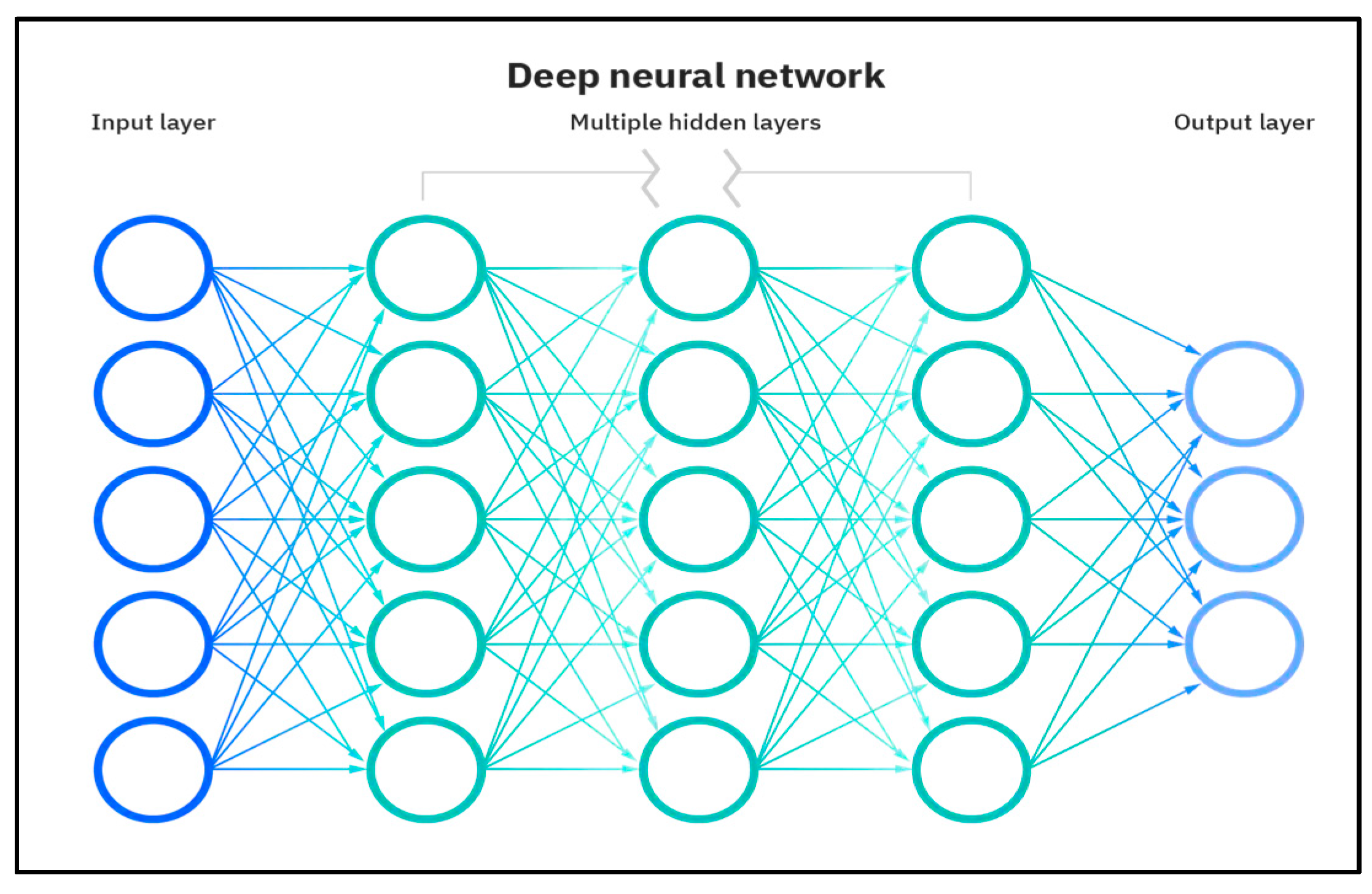
Figure 1. The architecture of an artificial neural network.
Asi 06 00106 g001
Figure 2. Unfolded recurrent neural network.
Asi 06 00106 g002
Figure 3. LSTM architecture.
Asi 06 00106 g003
Figure 4. The reinforcement learning process.
Asi 06 00106 g004
Figure 5. The DRL process.
Asi 06 00106 g005
Figure 6. The architecture with components of the proposed stock prediction model.
Asi 06 00106 g006
Figure 7. The architecture of VMD plus LSTM.
Asi 06 00106 g007
Figure 8. Plot for accuracy rate from models.
Asi 06 00106 g008
Figure 9. Actual prices vs. predicted prices.
Asi 06 00106 g009
Figure 10. Graph showing metrics for annualized wealth rate.
Asi 06 00106 g010
Figure 11. Graph showing the comparison of metrics for the average maximum drawdown algorithm.
Asi 06 00106 g011
Figure 12. Effect of using the sentiment analysis module.
Asi 06 00106 g012
Table 1. Findings on gold data using sentiment analysis.
ModelAccuracyRemarks
TFIDF + ANN85%Base Model
BERT + ANN96.2%11.2% improvement over the base model
TFIDF + BERT + ANN96.8%0.6% improvement over BERT + ANN
Table 2. VMD hyperparameters.
ParameterDescriptionValue
αModerate bandwidth constraint5000
τNoise tolerance with no strict fidelity enforced0
kmodes5
DCDC part is not imposed0
initWill initialize all omegas uniformly1
tol1 × 10−7
Table 3. LSTM Parameters.
ParameterValue
Learning rate0.001
Input size5
Hidden size200
Number of epochs2000
Number of layers2
Table 4. Hyper-parameters adopted in the implemented DRL algorithm.
ParameterValue
Discount0.99
Epsilon max1.0
Epsilon min0.01
Epsilon decay0.001
Memory capacity5000
Learning rate1 × 10−3
Action size4
Input layerInput size × 1000
Hidden layer1000 × 600
Output layer600 × output size
Table 5. Accuracy of model performance.
MetricsBest StockBuy and Hold(CRP)Proposed Algorithm
average_profit_return0.00110.00110.00110.01
Sharpe ratio2.52.42.43
Average maximum drawdown0.00310.020.010.03
Calmar ratio6.12.633
Annualized return rate (ARR)0.50.50.51.1
Annualized Sharpe ratio (ANSR)47.8474757.2
Table 6. Accuracy of price prediction phase.
MetricTraining DataTest Data
With VMDW/O VMDWith VMDW/O VMD
MAE3.644.14.35.6
MSE20.526.131.656.9
MAPE0.290.330.330.43
Disclaimer/Publisher’s Note: The statements, opinions and data contained in all publications are solely those of the individual author(s) and contributor(s) and not of MDPI and/or the editor(s). MDPI and/or the editor(s) disclaim responsibility for any injury to people or property resulting from any ideas, methods, instructions or products referred to in the content.