Article

The Method of Restoring Lost Information from Sensors Based on Auto-Associative Neural Networks

by
Serhii Vladov
1,
Ruslan Yakovliev
1,
Victoria Vysotska
2,3,
Mariia Nazarkevych
2,* and
Vasyl Lytvyn
2
1
Department of Scientific Work Organization and Gender Issues, Kremenchuk Flight College of Kharkiv National University of Internal Affairs, 17/6 Peremohy Street, 39605 Kremenchuk, Ukraine
2
Information Systems and Networks Department, Lviv Polytechnic National University, 12 Bandera Street, 79013 Lviv, Ukraine
3
Institute of Computer Science, Osnabrück University, 1 Friedrich-Janssen-Street, 49076 Osnabrück, Germany
*
Author to whom correspondence should be addressed.
Appl. Syst. Innov. 2024, 7(3), 53; https://doi.org/10.3390/asi7030053
Submission received: 22 March 2024 / Revised: 4 June 2024 / Accepted: 12 June 2024 / Published: 20 June 2024
(This article belongs to the Section Information Systems)

Abstract

:
The research aims to develop a neural network-based lost information restoration method when the complex nonlinear technical object (using the example of helicopter turboshaft engines) sensors fail during operation. The basis of the research is an auto-associative neural network (autoencoder), which makes it possible to restore lost information due to the sensor failure with an accuracy of more than 99%. An auto-associative neural network (autoencoder)-modified training method is proposed. It uses regularization coefficients that consist of the loss function to create a more stable and common model. It works well on the training sample of data and can produce good results on new data. Also, it reduces its overtraining risk when it adapts too much to the training data sample and loses its ability to generalize new data. This is especially important for small amounts of data or complex models. It has been determined based on the computational experiment results (the example of the TV3-117 turboshaft engine) that lost information restoration based on an auto-associative neural network provides a data restoring error of no more than 0.45% in the case of single failures and no more than 0.6% in case of double failures of the engine parameter registration sensor event.

1. Introduction

During the operation of a complex nonlinear technical object, its parameters are continuously monitored to determine its actual state. It is known that the data synchronization unit constantly records and analyzes a parameter set. This characterizes the dynamics of a nonlinear technical object and a discrete parameter set (including discrete ones). For example, more than 3500 parameters are recorded in the database (DB) per hour of a nonlinear technical object operation. In these conditions, failures of the control and measuring reliability equipment, especially sensors, in the control system of a nonlinear technical object [1,2] lead to serious consequences (15 to 20% of nonlinear technical object failures are associated with the sensor’s failure [3,4]). It is related to early completion of work or premature decommissioning of the facility. A sensor malfunction in one of the measuring channels is the most significant failure, which can be short-term or long-term. For example, the gas generator rotor r.p.m. sensor failure in helicopter turboshaft engines (TE) can lead to the false signal output from the speed controller to increase fuel consumption (fuel pump–dosing needle) [5,6] to the engine combustion chamber. This, in turn, can lead to its destruction (the combustion chamber walls burning) or the thermal destruction of the turbine blades. Therefore, the dynamic monitoring and operation management system of a complex nonlinear technical object (including helicopter TE) should produce high resistance to failures. This is ensured during the failure state detection, failure localization, and operability restoration.
One of the key tasks of a complex nonlinear technical project operation management is the parametric failure detection of sensors (degradation of their characteristics). In this case, as a rule, the majority control method can be used [7]. It consists of the fact that if one of the sensors has a characteristic different from the reference one, the additional measurement channel introduction in the mathematical model form allows for calculating the average value of this measurement (median) and, thereby, restoring the information lost from the sensor. The solution to the information restoration task using a neural network model of the engine is decomposed into two sub-problems: the mathematical model identification problem and the information restoration problem. The solution to the information restoration problem using neural network technologies (given in [7]) is directly related to the sensor failure detection and the lost information restoration based on neural network methods and engineering techniques through the following implementation steps: statistical data processing (preprocessing stage); choosing the architecture of the neural network and its structure; the neural network training algorithm selection; neural network training; neural network testing; and the neural network work efficiency evaluation [8].
One of the neural network methods to solve the lost information restoration problem is based on a neural network as a mathematical model of a complex nonlinear technical object (for example, helicopter TE), obtained during its characteristics identification process. In [9,10], the lost information restoration possibility from aircraft gas turbine engine (GTE) sensors is stated, but at the same time, there is no method based on which the lost data are restored. In [11], a technique for the lost information restoration process from GTE sensors as part of the onboard system for monitoring and diagnosing its operational status was proposed and software was created.
The analysis shows that the task range that needs to be solved is constantly growing. This is explained by the constant improvement of complex nonlinear technical objects (including helicopter TE) and, as a result, the functions they perform, as well as the corresponding increase in the number of controlled and diagnosed parameters [12]. Nevertheless, concurrently tackling a diverse array of tasks presents inherent challenges: constraints stemming from limited computational resources, such as RAM capacity, processing speed, and result precision; complexities in formalizing traditional control and diagnostic algorithms, thereby impeding their practical application; the imperative to execute aforementioned algorithms in a low-level language like assembler; and complications in data restoration in the sensor malfunction event.
Another alternative approach to information restoration is using the autoencoder (auto-associative neural network, ANN), which is characterized by compression and subsequent information restoration. Works like [13] show the ANN use possibility to restore measured information based on known object parameters. This approach’s disadvantage is a high error of single failure restoration of the onboard system for monitoring and diagnosing sensors—the value restoration error from the sensors in the break event is 4.5 to 5.0%, and in the gradual failure case, it is up to 5.5%.
Another approach to restoring lost information from an onboard system for monitoring and diagnosing sensors based on an ANN is to use a buffer (memory stack) to store the last valid value from sensor failures. This approach was considered in [14], where, in contrast to [9,10], a method for determining the optimal size of the ANN shaft was studied. However, there was no engineering method for obtaining a working ANN for the lost information restoration process from the onboard system for monitoring and diagnosing sensors. The principal component method research makes it possible to build an optimal ANN structure, the use of which to solve this task reduces the lost information restoration error from sensors.
ANN has become widespread in object-tracking systems [15]. Their use allows us to effectively solve object detecting and tracking problems in real time by automatically studying and extracting important features from input data, such as a video stream or an image. ANNs can display complex relationships in objects and their changes, providing high tracking accuracy [16]. The research results [16] are of great interest for the development of control and information processing systems for computer vision and image analysis. They are especially valuable for tasks that involve determining the spatial parameters of imaged objects, opening up new opportunities for improving system tracking and object recognition in real time. This is especially relevant in the autonomous systems technologies’ development context [17] where accurate spatial determination of object characteristics is key to effective functioning. For example, the ANN application in real-time object tracking systems can improve autonomous vehicle navigation, in particular, helicopters. They can effectively respond to environmental changes and avoid obstacles. And the smooth functioning of their engines will lead to safe flight. Such innovations for tracking objects with the ANN open new horizons and promote automated system development, which is important in the modern world where artificial intelligence technologies are becoming an indispensable part of everyday life.
It is also worth stating how useful the ANN is in face recognition tasks in video sequences [18]. The ANN application allows us to effectively solve challenges related to dynamic changes in position, lighting, and facial expressions in real time. ANNs can automatically train and adapt to face variations, using an encoder to compress information and a decoder to reproduce the original images. This contributes to increasing the face recognition accuracy in changing context and video sequence dynamics conditions. It makes ANNs effective tools for real-time face tracking and identification system development.
For example, in [19], an ANN was tested based on the ORL database. It included face images with slight changes in lighting, scale, spatial position, orientation, and various emotional expressions with a high recognition accuracy of 96%. This shows the significant performance of an ANN under the context change and variation conditions in image parameters, indicating their potential importance in real-time face recognition and identification tasks.
Based on the above, it can be stated that ANNs can be used for information restoration tasks. This direction is closely related to object tracking and recognition because they all describe working with incomplete or damaged data. After analyzing [15,16,17,18,19], information restoration tasks examples using ANNs were systematized:
  • Image restoration: ANN can be used to restore damaged or incomplete images, such as those with noise, compression artifacts, or blur.
  • Denoising algorithms can sometimes smooth out not only noise but also fine details in the data, and other types of denoising can lead to blurring where sharp edges and textures are lost, making the data less accurate. ANNs can be used to remove noise from images or signals.
  • Interpolation can create false patterns or structures that do not exist in the original data. ANNs can be used to fill in gaps in data, for example, to create higher-resolution images.
  • Super resolution: ANNs can enhance low-quality image fidelity.
At the same time, the ANN has the following advantages for information restoration tasks:
  • Efficiency: ANNs can be very efficient compared with traditional information restoration methods.
  • Flexibility: ANNs can be adapted to different types of data and tasks.
  • Training: ANNs can automatically train from examples, making them more robust to noise and other data corruption.
The lost information restoration task set in this work is relevant taking into account the above. It consists of the fact that in the modern technical progress conditions and the technical systems’ complexity, ensuring their reliability and uninterrupted functioning becomes critically important. Because sensor failures are one of the common causes of accidents and system failures, the development of effective dynamic control and monitoring systems becomes an urgent need.
This research aims to develop a complex nonlinear technical object system (including helicopter TE) for monitoring and operation control. It will ensure the lost information restoration in case of sensor failure. This will ensure the object’s operation continuity and reliability in abnormal situations. The research’s main tasks include the measured data analysis and processing using nonlinear dynamics methods for accurate monitoring and the method development for rapid detection and localization of sensor failures. Also, this will create the system that quickly restores the sensor’s performance to ensure the uninterrupted operation of the facility.
The research results are relevant for applied system innovation development by offering a new method for solving the information restoration task when sensors fail. The research results will be relevant to researchers, engineers, and developers of complex management and control systems, industrial automation, robotics, intelligent systems, information technology, cybersecurity, etc., using applied system innovation.
The scientific novelty of the obtained results is the development of a neural network method for lost information restoration in complex dynamic object sensor failure cases, which, through the auto-associative neural network (autoencoder) use, makes it possible to restore lost data in sensor failures with almost 100% accuracy.

2. Related Work Discussion

Today, the lost information restoration task when complex dynamic object sensors fail is relevant and widespread since sensors are widely used to collect data in various systems, including aviation, medicine, manufacturing, and much more. If a sensor fails or malfunctions [20,21], it can lead to valuable information loss, which can lead to system failures or even accidents. Therefore, lost information restoration in such cases becomes a critical issue to ensure the system’s reliable operation and everyone’s safety.
To solve this task, it is necessary to carefully select and modify the neural network structure, develop effective methods for training them, simulate various sensor failure scenarios, and compare the proposed solutions with existing methods. This will identify improvements and ensure that systems operate reliably while minimizing risks to safety and efficiency.
Ref. [22] shows the restoration possibility for the incomplete, damaged, or missing audio signals caused by numerous unforeseen situations, one of which is the sensor failure (audio signal receiver). Restoring incomplete, damaged, or missing audio signals is proposed to be solved as a time series forecasting problem using long short-term memory (LSTM) networks. The LSTM networks’ disadvantage in solving the incomplete, damaged, or missing lost information restoration problem when sensors fail is their limited ability to capture long-term dependencies in the data, which can lead to ineffective restoring of the complex dynamic object combined lost information in their operating mode.
In [23], a distributive training method is proposed for communication coherence restoration in the controlling multiple agents’ process using a linear neural network, the training of which is based on the adaptive control principles, within which the neural network strives to implement an anti-gradient value determined by the distances between agents and their neighbors. This approach’s disadvantage is the limited ability of a linear neural network to effectively respond to dynamic changes in the connection profile of a mobile multi-agent system and to ensure reliable restoration of communication under significant speed disturbances, which is critical in the complex dynamic object operation.
Ref. [24] researched situations where data are provided in a rounded form, with rounding errors comparable to or greater than measurement errors. Also, this study explored possibilities of achieving greater accuracy than the sampling step and lost information restoration using additional measurement errors. The proposed approach’s disadvantage to the complex dynamic object operation is the information restoration accuracy limitation when significant changes in the object or the environment parameters can reduce the system monitoring and control efficiency in real time.
In [25], restoring the sign bits task of DCT coefficients in digital images is solved as a mixed integer linear programming problem using two special properties of natural images. The proposed information restoration method accuracy did not exceed 1%. Despite the high accuracy of the proposed method, its disadvantage in the complex objects’ operation is its limited applicability in real conditions, for example, helicopter flight mode, which may not be enough for effective monitoring and control of complex dynamic objects.
Ref. [26] proposed approximate methods for the complete regression equation restoration in various situations for forecasting models where there are incomplete data based on the binary logistic regression use. The disadvantage of using binary logistic regression to restore lost information when sensors fail on complex dynamic objects may be the insufficient ability of the model to take into account complex relations and dynamic changes in the system, which can lead to insufficient accuracy of data restoration. In such cases, it is advisable to consider an ANN use [27,28,29], which is capable of extracting more complex and abstract features from data, taking into account their dynamic features and providing more accurate information restoration in the sensor failure event.
The ANN [27,28,29] used in the lost information restoration task, including multimedia data, the advantages of which include the ability to highly compress data samples, efficient use of memory, the ability to fill missing data and generate said data for better analysis of incomplete data, as well as lower training and clustering time compared with most clustering algorithms, becomes suitable for use on low-performance equipment with limited computing power and memory, which is relevant when operating complex dynamic objects. However, to improve the ANN’s ability to extract and represent a lot of complex and abstract features from data, as well as to ensure a better ability of the model to restore and generate information, especially in cases with incomplete data or high dimensionality, it is advisable to modify the traditional algorithm for training it, which is based on gradient descent.
Ref. [30] considers the training data restoration problem from overparameterized ANN models. The ANN used was trained on a specific training data set to implicitly take into account this data set features when reconstructing information. We explore various deep ANN structures, including fully connected and U-Net, with different activation functions and training loss function values. We demonstrate that the method significantly outperforms previous approaches for data restoration from autoencoders. This approach’s disadvantage is the need to take into account the degraded training sample and formulate the original sample restoration as an optimization problem, which requires complex calculations and estimates of the unknown degradation operator, which can reduce the method’s effectiveness in practical operating conditions of complex dynamic objects.
The article [31] proposed a technique for the automatic interpretation of distributed fiber optic sensor (DFOS) data for pipeline corrosion monitoring using machine learning. The machine learning model detects corrosion in real time, and the corrosion quantification method is based on the model data. The approach’s effectiveness is confirmed by laboratory tests that take into account pipeline diameter, DFOS spatial resolution, optical fiber type, and sensor installation methods. The results show high values of the F1 metric of 0.986 and the determination coefficient of 0.953. The key disadvantage of [31] is the high dependence on the original data quality, which can be eliminated based on an autoencoder to improve the data representation and reduce noise.
The closest to the method proposed in this work for lost information restoration in the complex dynamic object sensor failure event under operating conditions using an ANN is the method developed by Zhernakov and Musluhov in [9,10,11] for information restoration in the sensor failure event using an ANN, by compressing input data in its hidden layer, the shaft, and performing restoration in the output layer. One of the key disadvantages of this method is that the ANN structure choice is carried out based on the minimum error in the ANN information restoration from the neuron number in the “shaft”, which may be insufficient for the effective extraction and representation of complex features in the data. Another disadvantage is the traditional ANN training method based on gradient descent without regularization, which increases the model’s overtraining risk when it becomes strongly adapted to the training data and loses the ability to generalize new data. Even though the maximum error in lost information restoration did not exceed 0.58%, the solution accuracy for ANN lost information restoration on the test data set was 0.901 (90.1%) under operating conditions of complex dynamic objects, and the obtained indicators were high, there is potential to further improve the lost information restoration efficiency by optimizing model parameters or making adjustments to its structure.
Thus, based on the extensive discussions of related works [26,27,28,29,30,31]—in particular, the closest approximation to the method proposed in the work for lost information restoration in the complex dynamic object sensor failure event under operating conditions using an ANN [9,10,11]—to achieve the study aim, the key issues addressed in this work are as follows:
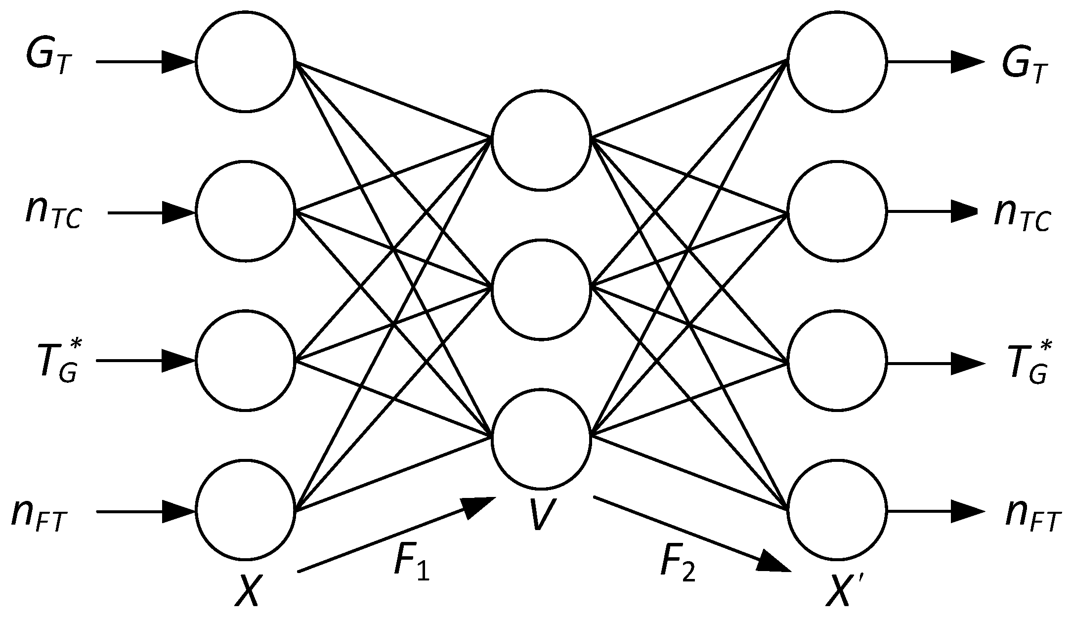
  • Choosing an ANN structure to solve for effectively extracting and representing complex feature task in data;
  • The traditional ANN training method modification based on gradient descent by adding regularization to reduce the model overtraining risk when it is strongly adapted to the training data and loses the ability to generalize new data;
  • Training the ANN on the test set with the loss function analysis at the training and model validation stages;
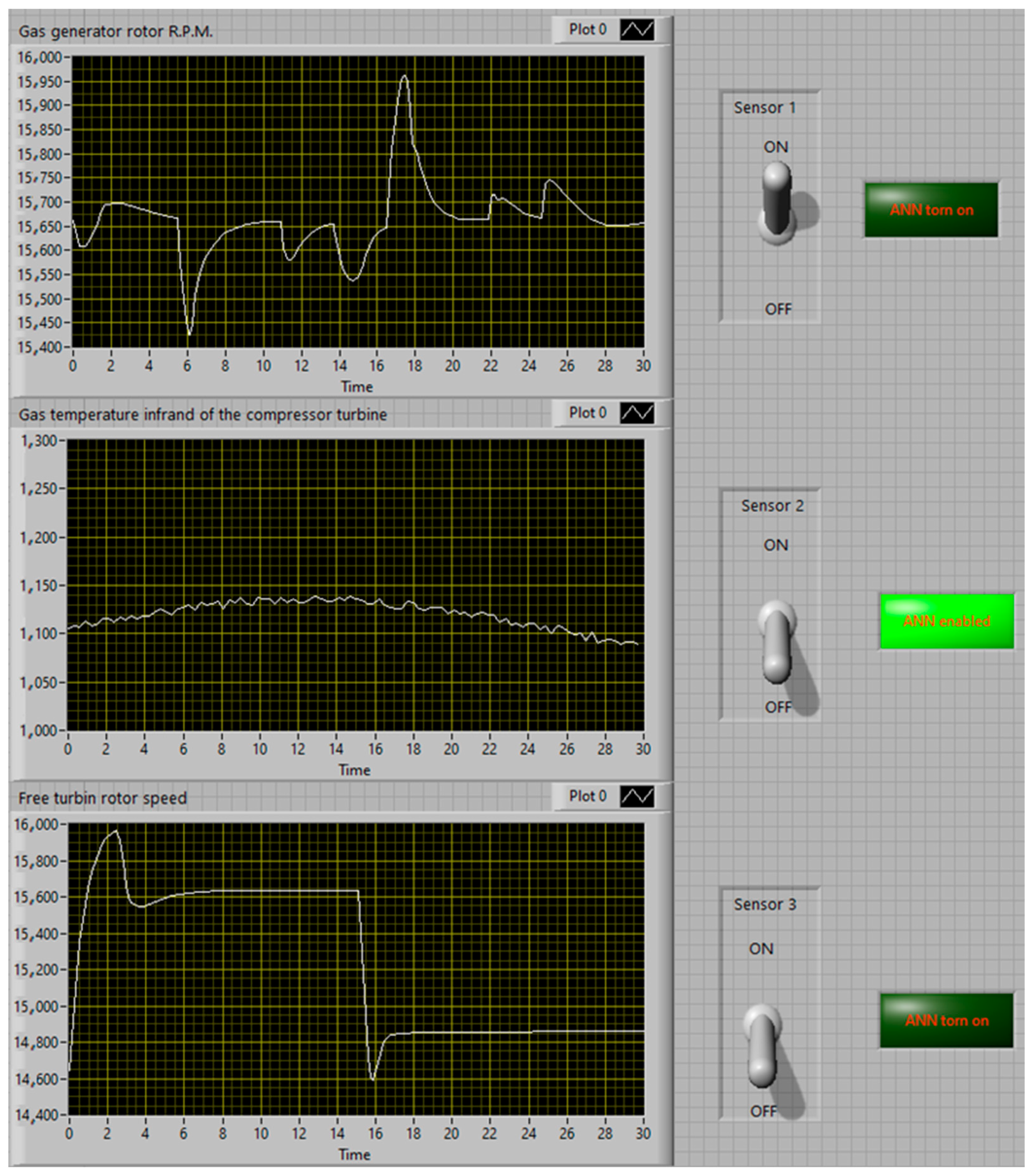
  • Carrying out a computer simulation of the failure situation of complex dynamic object sensors (the TV3-117 TE example used).
  • The failure results from modeling comparison for complex dynamic object sensors (using the example of the TV3-117 TE) with the results of the most approximate method [9,10,11] and highlighting its main advantages.

3. Materials and Methods

This work considers the TV3-117 TE As a research object for the helicopter’s TE class. The work considers the following task: it is required to build and train an ANN that provides information monitoring and restoration (in failure case) about the complex nonlinear technical object (the TV3-117 TE example using) operational status in the N standard sensors presence. In this case, the ANN performs a mirror image of the input data vector onto itself. Information compression is carried out in the hidden layer of the ANN, called the “shaft”, and information restoration is in the output layer. The fundamental possibility of using compressive mapping forms the principal component method basis [9,10,11,32,33]. The ANN architecture is shown in Figure 1.
The key point in choosing the ANN structure is determining the optimal number of neurons in the hidden layer [9,10,11,34]. For example, Figure 2 shows the error dependence in information restoration by the ANN [32,33,34] in the failure event of one of the sensors (for example, a TV3-117 TE gas generator rotor r.p.m. [35,36]) on the neuron number in the ANN shaft, calculated according to the expression:
M S E = 1 n · x d e c e n c x 2 ,
where x is input data, enc(x) is hidden layer output (encoded data), dec(enc(x)) is reconstructed data, and n is the example number in the training set.
The abscissa axis in Figure 2 shows the relative size of the shaft—the neurons’ number ratio in the shaft to the input/output neurons’ number (5 neurons). The optimal shaft size in this case is 0.8 (Figure 2). That is, the neurons’ number in the shaft (ANN hidden layer) should be 0.8 × 5.0 = 4.0. Data for ANN training during flight tests of the TV3-117 TE in a wide range of changes in operating modes (from low throttle to emergency mode) are obtained.
Along with the ANN structure chosen, an important stage is an information restoration stage based on this neural network functioning results. This work uses the approach proposed in [10,11], and it is shown in Figure 3.
Signals from the sensors are simultaneously sent to the stack and the tolerance control system, which monitors the measured values from the sensors. If the signals from the sensors are within the tolerance field, they are transmitted further to the control system, which manages the executive mechanisms (EM) affecting the object. If any of the sensor signals goes beyond the tolerance field, then, the tolerance control system removes the last value of this signal from a stack and transfers it to the corresponding input ANN, which restores the information and then transmits it to the automated control system (ACS).
The information restoration process from sensors based on an ANN occurs according to the functional scheme presented in Figure 4. The ANN is included directly between the S1...Sn sensors (or in the common information channel) and the ACS.
The proposed functional scheme advantages (Figure 4) are the implementation simplicity and the ANN work transparency as part of the management system. To calculate the lost information restoration error from the sensors, the form dependence is used [9]:
e = r e a l v a l u e n w a v a l u e m a x v a l u e m i n v a l u e · 100 % ,
where r e a l v a l u e is the real value of the parameter; n w a v a l u e is the restored parameter value; m a x v a l u e , m i n v a l u e are the maximum and minimum values of the parameter.
In the presented work context, which considers the ANN use to monitor and restore information about the complex nonlinear technical object state, improving the ANN training algorithm is critical. The training algorithm directly affects the network’s ability to adequately respond to changes in data, including sensor failures, which is important to ensure the object’s safety and stability. Thus, improving the ANN training algorithm includes several aspects:
  • Improved adaptability, which implies the algorithm’s ability to adapt to changes in object operating conditions, including operating modes changes and possible abnormal situations;
  • Improving generalization ability, which means that the network needs to undergo training not just on data collected during tests but also on possessing the ability to generalize its acquired insights to adapt to unforeseen scenarios encountered in real-world operations;
  • Accounting for process dynamics, which requires the training algorithm to take into account the engine state dynamics and the corresponding dynamics data coming from the sensors;
  • Improving noise and error tolerance, which requires the network’s ability to operate effectively even in the data noise or errors presence in sensor measurements;
  • Training time optimization, refers to reducing the training time required by a network to improve its efficiency and practical applicability.
Thus, the approach to improving the training algorithm should be comprehensive, including both theoretical developments and practical experiments with various training methods and network architectures. This approach will help ensure optimal operation in the system for information monitoring and restoration of the object condition in a wide range of operating conditions.
Using the basic ANN training algorithm, a modified method for training is proposed by adding regularization to the loss function and updating the weights to achieve the following goals:
Goal 1. Prevent overfitting. Regularization helps reduce the model overfitting risk where it overfits the training data and loses its ability to generalize new data. This is especially important for small data volumes or complex models.
Goal 2. Improve generalization ability. We try to create a more robust and generalizable model by adding regularization to the loss function. The model not only performs well on training data but can also produce good results on new data.
Goal 3. Control the model complexity. Regularization helps control the model complexity by the weights and their growth restraining. This allows for simpler and more interpretable models, which is often a desirable property in practical applications.
Goal 4. Improve training robustness: Adding regularization can help improve the training process stability by reducing the model sensitivity to changes in training parameters or input data.
Below is a step-by-step description of the proposed modified ANN training algorithm with the regularization addition to the loss function and updating the weights.
Step 1. The ANN weights are the initialized data with random values. Let us denote the weight matrix W(l) between layer l and l + 1.
Step 2. Next, the input data x is fed to the input layer, and activation a(0) = x is carried out. For each layer l, we can write:
z l + 1 = a l · W l + b l ,
a l + 1 = f z l + 1 ,
where f is the activation function and b(l) is the displacement vector on layer l.
Step 3. At this stage, the resulting output a(L) is compared with the input data x using the loss function L according to the expression:
L x , a L = 1 2 · n · i = 1 n x i a i L 2 + λ 1 · l i , j W i j l + λ 2 · l i , j W i j l 2 ,
where n is the input data elements number and λ1 and λ2 are the regularization coefficients for L1 and L2, respectively.
Step 4. Applying the chain rule to calculate the loss function gradients over the ANN parameters, the network weights and bias are updated using gradient descent:
= α · L W i j l ,
b j l = b j l α · L b j l .
Steps 2–4 are repeated for each training epoch or until a stopping criterion is reached (e.g., decreasing the loss function to a certain threshold).
Using the proposed ANN training algorithm, a hypothesis is proposed for updating the weights in the ANN using gradient descent with L1 and L2 regularization:
Hypothesis 1.
When using gradient descent with L1 and L2 regularization to update the auto-associative neural network (autoencoder) weights, the network weights will be updated as follows:
W i j l = W i j l α · L W i j l + λ 1 · s i g n W i j l + 2 · λ 2 · W i j l .
Proof of Hypothesis 1.
Let W i j l be the weight between neurons i and j on layer l, α be the training rate, and λ1 with λ2 be the regularization coefficients of L1 and L2, respectively. According to the gradient descent algorithm with L1 and L2 regularization, the weights are updated according to the following expression:
W i j l = W i j l α · L W i j l α · λ 1 · s i g n W i j l 2 · α · λ 2 · W i j l .
Next, the partial derivatives of the loss function for the weights for updating are derived:
L W i j l = L a l · a l z l · z l W i j l .
After loss and activation functions derivatives substitution, the following expression is obtained:
W i j l = W i j l α · 1 n · a L x · f z L · a L + λ 1 · s i g n W i j l + 2 · λ 2 · W i j l .
Thus, according to (11), the ANN weights were updated taking into account the loss function gradient and the L1 and L2 regularization. The derivation of this proof of the hypothesis shows updated ANN weights when using gradient descent with L1 and L2 regularization. In particular, it can be seen that updating the weights includes three components:
  • The loss function gradient over the weights, which is responsible for correcting the weights taking into account the error between the network output and the input data;
  • L1 regularization, which penalizes the absolute value of the weights, helps in reducing the model complexity, and prevents overfitting;
  • L2 regularization, which penalizes the square of the weight and, also, helps the control model reduce overfitting and complexity.
Thus, updating the weights takes into account both the error in the data training and the two types of regularization, which helps in creating a more generalized and robust model. □
Regularization coefficients λ1 and λ2 must be set manually or selected using cross-validation or optimization methods:
  • Manually—λ1 and λ2 are selected by the expert or researcher based on their experience and intuition regarding the problem and data. If a more compressed model is required, then λ1 and λ2 can be chosen more strongly; if the model is prone to overfitting, then fewer may be selected.
  • Cross-validation is dividing the training data into several parts (folds), training the model on one part, and evaluating its performance on the remaining parts. The process is then repeated for different values of λ1 and λ2. The values that show the best performance on the test data are selected as optimal.
  • Optimization methods can used to automatically select the λ1 and λ2 values to minimize some target functionality, for example, the error in the validation set. This process may include optimization techniques such as grid search or surrogate model optimization algorithms.
Thus, when choosing values for λ1 and λ2, it is important to consider the balance between preventing overfitting and maintaining the information content of a model. Also, regularization values may depend on the data nature and size as well as the model complexity.

4. Results

After developing the ANN training algorithm, the next research stage involves a numerical experiment simulating the lost information restoration in the failure event of one of the standard sensors of the TV3-117 TE. The input variables of this model for helicopters TE consist of the atmospheric conditions—ρ is the air density, PN is the pressure, TN is the temperature, and h is the flight altitude—alongside onboard parameters: T G is the gas temperature in the compressor turbine front, nFT is the free turbine rotor speed, nTC is the gas generator rotor r.p.m., and GT is the fuel consumption, calculated according to [37,38,39] and normalized to absolute values using gas-dynamic similarity principles. It is presumed that atmospheric conditions remain constant throughout the analysis. Detailed analysis and preprocessing of input data (Table 1) are described in [37,38,39].
At the first stage of input data preprocessing, the Fisher–Pearson test value [40] is calculated based on the observed frequencies m1, …, mr (summing row by row the probability for each measured value result) and its comparison with the critical values of the Fisher–Pearson test χ2 with the freedom degrees number rk − 1. With the freedom degrees number rk − 1 = 13 and α = 0.05, the random variable χ2 = 3.588 did not exceed the critical value of 22.362, which means that the normal distribution law hypothesis can be accepted and the samples are homogeneous. The conclusion about the study sample homogeneity is confirmed based on the Fisher–Snedecor test [41]. The obtained result analysis shows that the larger dispersion ratio σ m a x 2 to σ m i n 2 , with the smaller one being 1.28 (less than the standardized critical value Fcritical = 3.44). Therefore, the sample training is homogeneous. To guarantee the training and testing data sets’ representativeness, a cluster analysis was performed on the initial data (Table 1), resulting in eight distinct class identifications (Figure 5a). After applying the randomization procedure, test and training (control) samples were formed in a 2:1 ratio (67 and 33%, respectively). The training and test sample (Figure 5b) clustering process [42,43] showed that both of them, like the control sample, consisted of eight classes. The distances between the clusters practically coincide in each of the considered samples, which indicates the test and training samples’ representativeness [37,38,39,40]. Thus, the resulting sample sizes were as follows: training—256 elements, control—172 elements (67% of the training sample), and test—84 elements (the training sample is 33%).
After the input data analysis and preprocessing, the ANN is directly trained. The ANN model is configured using the deep training libraries TensorFlow and Keras. In this model, the transmitter uses the ReLU activation function and the receiver uses the sigmoid function. The ANN is implemented using these typical deep learning Python libraries [44]. Table 2 shows the main ANN parameters for its training.
As the information restoration task solution attempt in the sensor failure event, a model experiment was carried out using an ANN, the results of which received 5062 values of the TV3-117 TE indicators (events), of which 4978 values were selected as favorable events and 84 as unfavorable events. Since there are few adverse events when training the model on this set, there is a high probability of the first kind of error (an incorrect value of the indicator is found to be correct). It is possible to train a model with the largest error shift to the second kind zone (the correct value of the indicator is recognized as incorrect). At the same time, the error will remain permissible. In this case, the admissible share of the correct values of the indicators will be calculated according to the universal mathematical GTE model with a free turbine [37,38,39]. In this research, it is assumed that the model is trained on favorable events. During training, the main component of the set is highlighted, and the dividing surface shifts to these set boundaries. If the model deviates above some threshold value, the event is considered unfavorable. The feature set, data preprocessing, and gap elimination methods are described in [37,38,39]. It is assumed based on works [45,46] that Y = (y1, y2,…, yp) is the feedback set about events, X i m = x 1 i , x 2 i ,   ,   x m i is the m feature set of the i-th event; Y 0 = y i = 0 y i Y ,   i = 1 , p ¯ is the favorable event class; Y 1 = y i = 1 y i Y ,   i = 1 , p ¯ is the adverse event class. The data amount after gap elimination and processing is n = 4 (the neurons’ number for input and output layers) and v = 3 as the neurons’ number for a hidden layer (“shaft”); Y 0 = 2893 , Y 1 = 66 . A duplicate set of features Xi  X i m = x 1 i ,   x 2 i ,     x m i was used as a teacher. That is, we obtained F :   X i X i , the classification task solving instead F :   X i y i . The ANN was trained on the set Y0 and the minimum training deviation for each output neuron was taken as the classification threshold. After ANN training, some test event yk was evaluated as: yk = 1 if a deviation above the threshold occurred in one of the output neurons; yk = 0 if the deviation on all output neurons did not exceed a threshold. The sigmoid activation function was used, and the loss function was the difference for each output neuron.
The test set consisted of 132 events (all Y1 events and, comparatively, 66 Y0 events). The training set consisted of 2827 events (all other Y0 events). The accuracy of 100% was achieved on the test set. When adding 12 insignificant features [45,47], a 99.53% accuracy was achieved where 0.47% was a second-order error (4 valid values of an indicator were recognized as incorrect). It is noted that the results were obtained on the relatively small test set. Objective verification requires access to a larger volume of adverse events and different stages of repeated testing.
It is assumed that V is the hidden layer neuron set. At the same time, in the ANN (Figure 1),
F 2 V : F 1 1 X + ε n ,
where εn = (ε1, ε2, ..., εn) is the training error.
It is considered that the ANN has completed training if εn = σn where σn = (σ1, σ2, ..., σn) insurmountable training error [45]. The hidden layer V of a smaller dimension amplifies the values that allow for the inverse mapping of F2(V) with the smallest error ε n σ n and attenuates the values that introduce noise. Then F2(V) at εn = σn is the main component of the set Xn (Figure 6).
The test event yk classification is possible on the error plane due to the deviation evaluation from the main component F2(V). Since the training was performed on the Y0 set, the deviation for Y1 events is expected to be higher. On the error plane, Y0 events will be concentrated in the zero zone, and Y1 will be distributed throughout space. Therefore, classification on the error plane will be simpler than on the feature plane (Figure 7).
Classification in the error space (Figure 7) can be implemented by separate methods, in particular, a threshold condition (Figure 8) of the form [45]:
1 , e j > σ j , e j e k , 0 , e j > σ j , e j e k .
The errors in the second kind are class Y0 outliers. A reduction in the emissions number is possible due to an increase in class Y0 data—the main component of the set will be formed more accurately. At the same time, it is easier to increase the data amount on the correct values of TV3-117 TE parameters than on abnormal ones. It should be noted that Figure 7 and Figure 8 show two-dimensional planes. When classifying in a multidimensional form, the error is much lower. The overtraining risk is extremely high when training ANNs of type F :   X i y i on a similar set. Since the Y1 data are much smaller than Y0, the separation surfaces can be distributed as in Figure 9 [45].
The ANN loss function dynamics [48] are analyzed at the stages for the model training and validation (Figure 10). This analysis provides a graphical representation of the change in loss function over time (training epochs number) for the validation and training data sets. Figure 10 allows us to evaluate the training model process and its generalization ability.
The obtained results of the loss function dynamics determined at the model validation and training stages allowed us to draw the following conclusions:
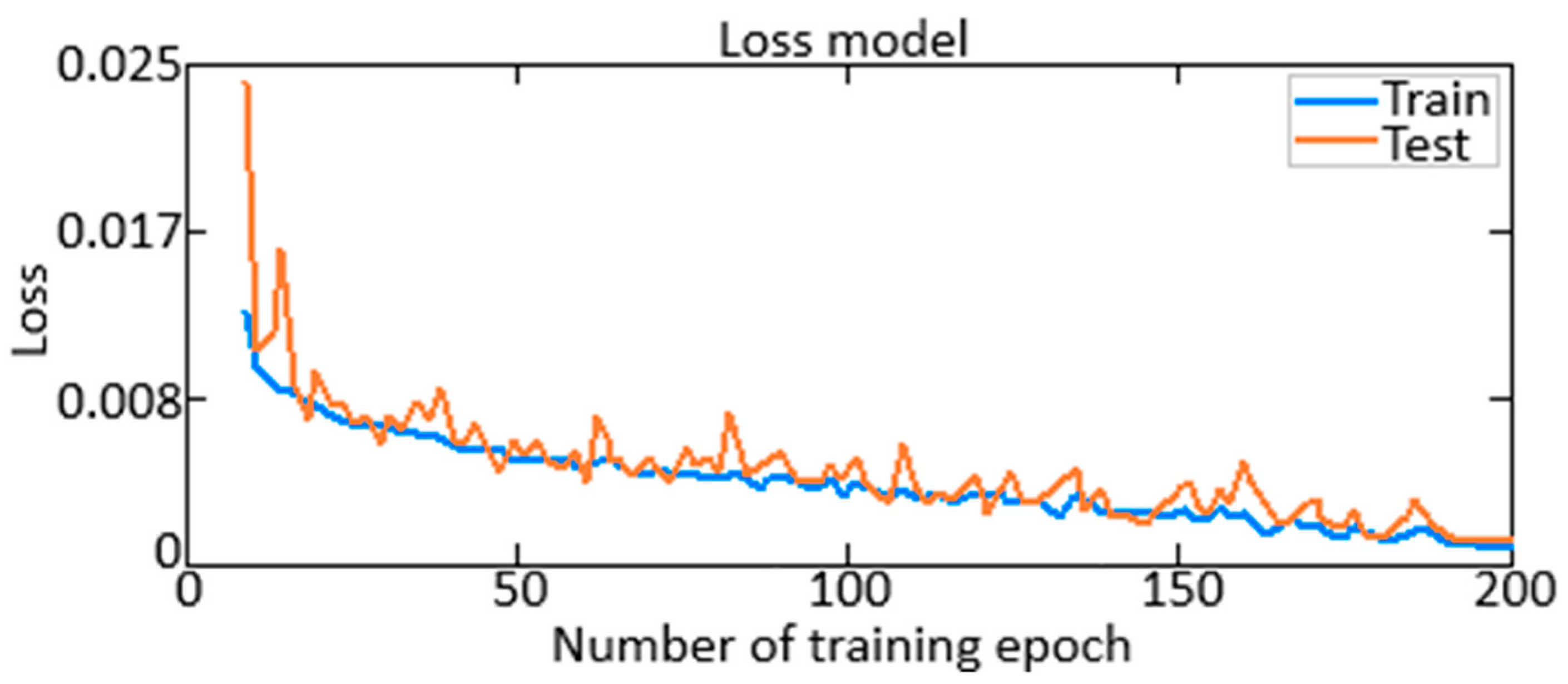
  • The loss function dynamics made it possible to evaluate the model training effectiveness. A decrease in the loss function on the training data set indicates that the model is successfully training and identifying patterns in the data. The loss function on the validation data set also decreases at the same time, which indicates the elimination of the overfitting effect.
  • The loss function dynamics comparison of the data set validation and training made it possible to assess the model generalization ability. Reducing the loss function on the validation and training data sets is also a pattern in the data. At the same time, the loss function on the validation data set also decreases, which indicates the overfitting effect elimination.
  • The loss function dynamics analysis also helped determine whether adjustments to training parameters such as training rates or regularization coefficients were required. Since the loss function is reduced on the training and validation data sets, changes to the training parameters may not be necessary to improve the ANN training process.
The work additionally assessed the Kullback–Leibler divergence [49] (Figure 11), which shows the information divergence (relative entropy) of two probability distributions and is calculated as follows:
D K L P Q = i = 0 N P x i · l o g P x i Q x i ,
where P(xi) is the original distribution and Q(xi) is the approximating distribution.
As can be seen in Figure 11, the maximum value of the deviation between two probabilistic distributions of the TV3-117 TE parameter values does not exceed 0.025 (2.5%) and does not exceed the maximum value of the loss function at the model validation and training stages, which is also 0.025 (2.5%); then, we can judge the acceptable divergence of probability distributions of the TV3-117 TE parameters.
To simulate the failure of one of the standard sensors of the TV3-117 TE, a virtual installation was created in the LabVIEW software package, which simulated a system with three sensors: gas generator rotor r.p.m. (D-2M), free turbine rotor speed sensor (D-1M), and gas temperature in the compressor turbine front (14 dual thermocouples T-102) (Figure 12).
Using the developed virtual installation, the LabVIEW software package simulated a single sensor failure (break), as well as the lost information restoration using an ANN. The lost information restoration diagram by the ANN in the failure event of one of the standard sensors of the TV3-117 TE (using the example sensor of the gas temperature in the compressor turbine front) is shown in Figure 13a; the lost information restoration process diagram from the onboard system for monitoring and diagnosing sensors of the “optimal“ ANN in a single failure case of the sensors (their disconnection) is shown in Figure 13b where the “white line” represents the parameter value, the “green line“ represents the restored signal value using the ANN, and the “red line“ represents the parameter value obtained from the sensor.
The approach disadvantage is proposed in Figure 13. There is a high error of value restoration in an onboard system failure case for monitoring and diagnosing one sensor: the restoration error is 4.5…5.0% in the case of an interruption and up to 5.5% in the gradual failure case. Another method of lost information restoration from sensors based on an ANN is the buffer (memory stack) used that stores the last correct value in the sensor failure case (Figure 13b). Experimental studies using the “optimal” ANN have shown that the lost information restoration error in the case of a single failure is 1.5…2.0% and, in the gradual failure case, does not exceed 2.5%. Additional error reduction is achieved by using a failure detection logic that identifies the failure and isolates the failed sensor.
To improve efficiency and reduce the lost information restoring error, new methods are used, improved based on the Zhernakov and Musluhov research [9,10,11]. In particular, the data from the sensors are constantly recorded in the buffer where the operating value is fixed when the sensor is active, and the restored value is used when it fails. The system automatically performs the following steps: receives output data from the sensors using the previous failed sensor parameter value from the buffer, sets the maximum number of calculations, initializes the calculation counter to 0, calculates the ANN outputs in the emulator, increments the calculation counter by 1, and transmits the management system result. At the same time, the proposed system envisages an additional neural network used to identify the complex dynamic objects’ parameters.
The proposed system is implemented as an improved functional scheme developed by Zhernakov and Musluhov in [9,10,11] in which the lost information from the sensors is automatically restored. When a sensor failure is detected, the integrated tolerance control system uses ANN calculations to write to the buffer (stack memory) (Figure 14).
If the sensor readings are outside the acceptable range, the tolerance control system declares the sensor as faulty and uses the last recorded value in the buffer to restore its value. Figure 15 shows the process diagram of restoring lost information from the ANN sensor of the TV3-117 TE (using the example sensor of the gas temperature in the compressor turbine front) based on the proposed (modernized) approach where the “white line” is the parameter value, the “green line” is the restored signal value using a neural network, and the “red line” is the parameter value obtained from the sensor. The information restoration error from the sensor in its interruption event and gradual failure does not exceed 0.25%.
According to Figure 13 and Figure 15, the information restoration error from the sensor in its interruption case and gradual failure does not exceed 0.25%. Therefore, it is recommended to use the Zhernakov and Musluhov methodology [9,10,11] for the neural network development, training, and testing for lost information restoration from sensors. This technique includes the following stages: data preprocessing (normalization, calibration, digitization) for neural network training; statistical processing of data to identify gross measurement errors; data scaling; the neural network architecture and structure choosing; shaft size determination based on the covariance analysis results using the principal components method; activation functions selection, training algorithm; neural network training; testing; and the developed neural network effectiveness evaluation in the process of restoring lost information from sensors. The ANN information restoration results in the gas temperature sensor event in the compressor turbine front of the TV3-117 TE in its failure event are shown in Table 3.
If other sensors fail, the restoring error does not exceed the values shown in Table 4. The obtained results analysis shows the high efficiency of ANN application in the information restoration process. Information restoration results in case of double (multiple) failures of nTC and T G sensors are shown in Table 4.
Table 3 and Table 4 analysis shows that the use of the ANN architecture 4–3–4 with the proposed improved method of its training as part of an improved functional diagram for information restoration (Figure 14) allows for 10% more accurate lost information restoration in the single failure (break) event of complex dynamic sensor objects (the TV3-117 TE example use) in comparison with the ANN architecture 5–4–5 as part of the basic functional information restoring diagram developed by Zhernakov and Musluhov [9,10,11]. Also, the use of the ANN architecture 4–3–4 with the proposed improved method of training it as part of an improved functional diagram for information restoring (Figure 14) allows for 14% more accurate restoration of lost information in the double (multiple) sensors failure event of complex dynamic objects (the TV3-117 TE example use) compared with the ANN architecture 5–4–5 as part of the basic functional diagram for information restoring developed by Zhernakov and Musluhov [9,10,11]. Increasing the lost information restoration accuracy by 10 to 14% is critical in the complex dynamic objects’ operation (for example, a TV3-117 TE in helicopter flight mode).
Analysis of the results given in Table 3 and Table 4 shows that even though the information restoration accuracy in the double sensor failures deteriorates somewhat, the ANN ensures satisfactory quality use of information restoration, i.e., the ACS measuring channel performance preservation.
Summarizing the obtained results, an engineering methodology for creating, training, and testing ANNs for restoring lost information from sensors is proposed, which includes the following steps: data preprocessing (normalization, calibration, digitization); statistical processing to detect gross measurement errors; data scaling; the ANN architecture and structure choosing; shaft size determination based on the covariance analysis results using the principal components method; activation functions selection, training algorithm; and the developed ANN effectiveness training, testing, and evaluating for lost information restoration from sensors.

5. Discussion

5.1. The Obtained Result Effectiveness Evaluation

The proposed ANN results with a modified training algorithm were assessed using the following metrics [51]:
-
Accuracy (precision);
-
Completeness (recall);
-
F-measure;
-
AUC (area under curve is the area under the ROC curve).
Precision is the measure of the proportion of accurately classified parameters relative to the overall count of true (both negative and positive) parameters [51]:
P r e c i s i o n = T P T P + F P ,
where FP is the false positive results and TP is the true positive results.
Recall is the fraction of the correctly classified parameters compared with the total count of parameters belonging to the true class [51]:
R e c a l l = T P T P + F N ,
where FN is the false negative results.
After calculating the “precision” and “recall” metrics values, a situation may occur in which the classifier’s recall is low and the precision is high. Therefore, it is necessary to introduce an additional metric, which is the harmonic mean of precision and recall, the so-called F-measure. This metric is calculated as follows [51]:
F m e a s u r e = 2 · P r e c i s i o n · R e c a l l P r e c i s i o n + R e c a l l .
The ROC (receiver operating characteristic) curve shows the trade-off between characteristics such as TPR (the real anomalies percentage that is correctly predicted by the classifier) and FPR (the real normal data percentage that is predicted as anomalous by the classifier). They are calculated as follows [51,52]:
T P R = T P T P + F N ,
F P R = F P T N + F P ,
where TN is the false negative result.
The area under the ROC curve is represented by the AUC metric, whose values range from 0.5 to 1. An AUC of 1 indicates that the model is ideal, and an AUC of 0.5 indicates that the model is guessing at random.
A comparison was made of the anomaly detection effectiveness using the proposed data set with various ANN models and classical machine learning methods. The obtained estimates are presented in Table 5, from which it follows:
  • The ANN recall and precision metrics, taking into account a slight imbalance in the data, are almost the same. Despite a slight imbalance, the support vector machine (SVM) managed to strike a harmony between precision and recall metrics, but it is still inferior to implemented autoencoders.
  • For the F-measure metric, a similar situation arises since the F-measure is the harmonic mean between the precision and recall. This metric shows that the linear regression method stands out from other methods in that it was unable to cope with the qualitative classification of both normal and anomalous data.
  • Analyzing the AUC-ROC value, it can be seen that the convolutional autoencoder showed the best performance, followed by the proposed ANN with structure 4–3–4. The SVM is only 10% inferior to the convolutional autoencoder due to its complex mathematical implementation and large classification penalties.
  • Despite the convolutional autoencoder superiority, this neural network type is much inferior to other algorithms in training time terms. With larger data and more layers in the decoder and encoder, this figure will increase significantly, so this autoencoder applicability may be reduced.
  • For anomaly detection, SVMs were optimized for comparison with autoencoders. From the obtained results, it is clear that after SVM optimization, its quality characteristics improved, but the training time increased 5 times.
Based on the research conducted, it turns out that despite the high-quality indicators of the optimized SVM, it is possible to obtain similar quality indicators from the proposed ANN with faster training.

5.2. The Obtained Results in Comparison with the Most Approximate Analog

The work provides a comparative analysis of the proposed method for restoring lost information with the closest one, which is based on an ANN with the traditional teaching method [9,10,11], developed by Zhernakov and Musluhov. Table 6 shows the main advantages of the proposed method over the closest one in terms of the following parameters: choice of ANN structure, ANN training method, maximum error in restoring lost information, restoring lost information task solving accuracy of each ANN on a test data set, training speed, generalization ability, use resources efficiency, and robustness.
The lost ANN information restoration task solving accuracy on a test data set is determined according to the expression:
A c c u r a c y = T P + T N T P + T N + F P + F N .
The generalization ability of an ANN evaluates its ability to correctly process new, previously unseen data. One way to evaluate generalization ability is to use a validation data set that was not used to train it. One measure of generalization ability is the difference between the error on the training data set and the error on the validation data set. If the error on the validation data set is comparable to the error on the training set, this may indicate good generalization ability. To assess the generalization ability, this work uses the determination coefficient R2 as a corresponding metric that evaluates how well the model fits new data and is determined according to the expression:
R 2 = i y i y ^ i 2 i y i y ¯ i 2 ,
where yi is the actual value of the target variable for the i-th example, y ^ i is the restored value of the target variable for the i-th example, and y ¯ i is the average value of the target variable across all examples.
The determination coefficient R2 ranges from 0 to 1. A value closer to 1 indicates that the model generalizes data better. A value closer to 0 or negative may indicate that the model is underfitted or overfitted.
To evaluate the ANN resources using efficiency, this work uses the Efficiency metric, which takes into account the predictions’ accuracy and the resources spent amount on training and/or prediction. One such metric could be the relationship between accuracy and resource utilization (for example, computational or time resources). It is assumed that Acc1 and Acc2 are the two ANN compared accuracies, and Res1 and Res2—resources used (the ANN training time parameter was used in this work since both networks were tested with an identical amount of memory—32 GB DDR-4). Then, the resource use efficiency assessment is determined by the expression:
E f f i c i e n c y 1 = A c c 1 R e s 1 ,       E f f i c i e n c y 2 = A c c 2 R e s 2 .
Thus, by comparing the effectiveness of two ANNs, it is possible to determine which of them demonstrates higher accuracy by the resources expended.
ANN robustness assessment can be achieved by analyzing its performance on different data sets or under different conditions. One of the approaches to solving the problem of robustness assessment is to research the change in the ANS reconstruction accuracy when varying the input data or model parameters. This work uses a traditional method for the ANN robustness assessment, which is based on determining the standard deviation of the lost information restoration accuracy on various subsamples or data sets—the smaller the standard deviation, the more resistant the ANN is to changes in data or conditions. The standard deviation of the lost information restoration accuracy is determined according to the expression:
σ = i = 1 N A c c i A c c ¯ 2 n ,
where Acci is the ANN accuracy on the i-th data set or with the i-th parameters variation, A c c ¯ is the average accuracy value for all observations, and n is the subsamples’ number.
In this work, for each ANS, the accuracy was determined on n = 8 different subsamples of 32 values in each training sample with a total volume of 256 values. It is assumed that Acc1i and Acc2i are the accuracy values of the first and second ANS on the i-th subsample, respectively (Table 7). Then the average accuracy for each neural network is, respectively, A c c 1 ¯ = 0.988 and A c c 2 ¯ = 0.901, and the average deviation—0.00524 and 0.01148.
Thus, the results obtained during the comparative analysis (Table 6) of the proposed method for restoring lost information with the closest one, which is based on the ANN with the traditional method of teaching [9,10,11], developed by Zhernakov and Musluhov, indicate that that the proposed method is more effective compared with [9,10,11] in performing the lost information restoration task during the sensor failure event in the operating mode of complex dynamic objects, for example, a TV3-117 TE in helicopter flight mode.

5.3. Results Generalizations

  • Further advancements have been made in refining the neural network approach for restoring lost data in the sensor failure event in intricate dynamic systems, which, through an auto-associative neural network (autoencoder) use, makes it possible to restore lost data with 99% accuracy. This is evidenced by the metrics of precision, recall, and F-measure, the values of which for normal data are 0.989, 0.987, and 0.988, respectively, and for abnormal data—0.967, 0.967, and 0.968, respectively.
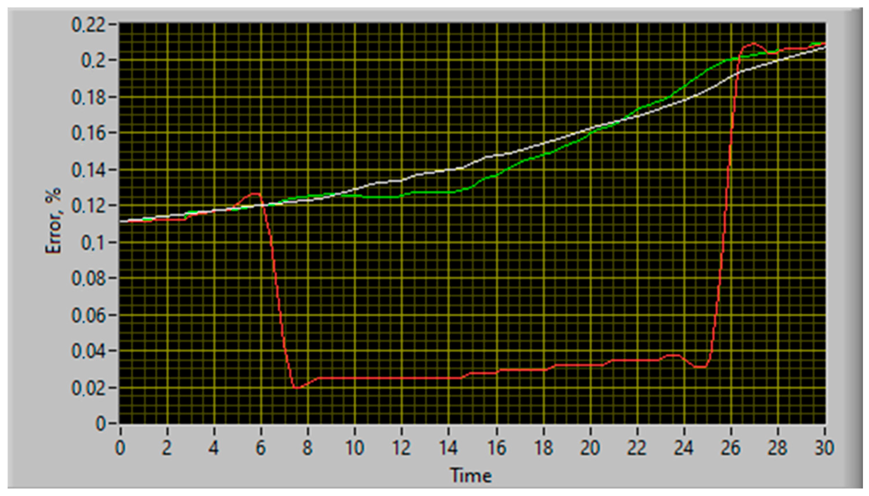
  • The basic training algorithm of an auto-associative neural network (autoencoder) has been improved by adding regularization to the loss function and updating the weights, which reduces the model overtraining risk when it adapts too much to the training data and loses the ability for new data generalization. It has been experimentally proven based on an improved training algorithm that an auto-associative neural network (autoencoder) indicates a minimal risk of model overtraining since the maximum value of the resulting loss function does not exceed 0.025 (2.5%).
  • For the first time, a hypothesis on updating weights in an auto-associative neural network (autoencoder) using gradient descent with regularization was formulated and proven, which confirms the basic training algorithm improving the feasibility of an auto-associative neural network (autoencoder) and, as a result, the model complexity controlling and reducing its risk of retraining.
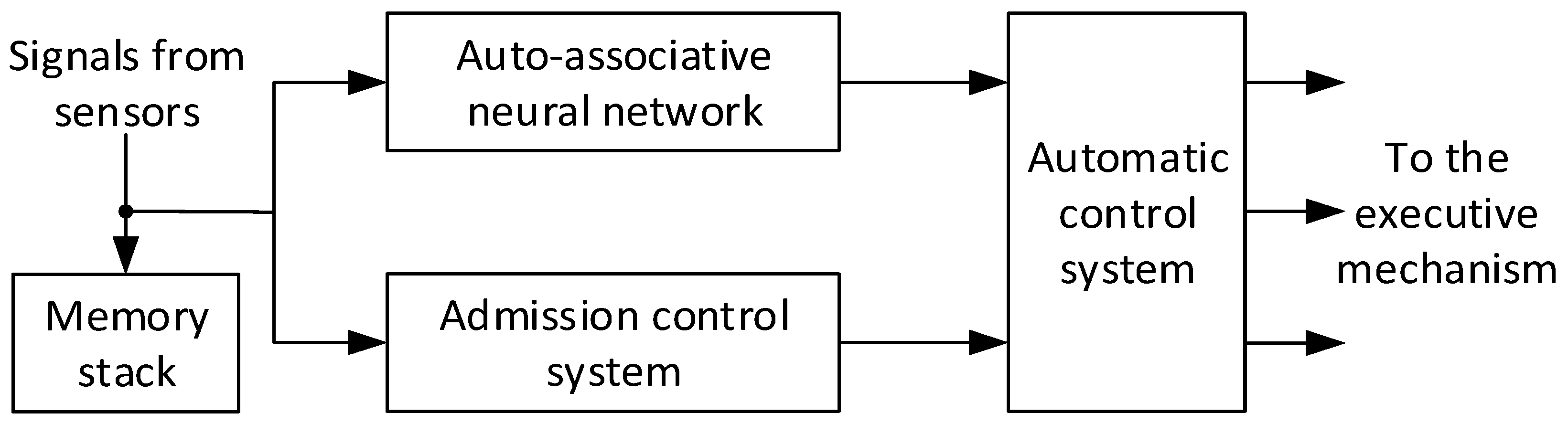
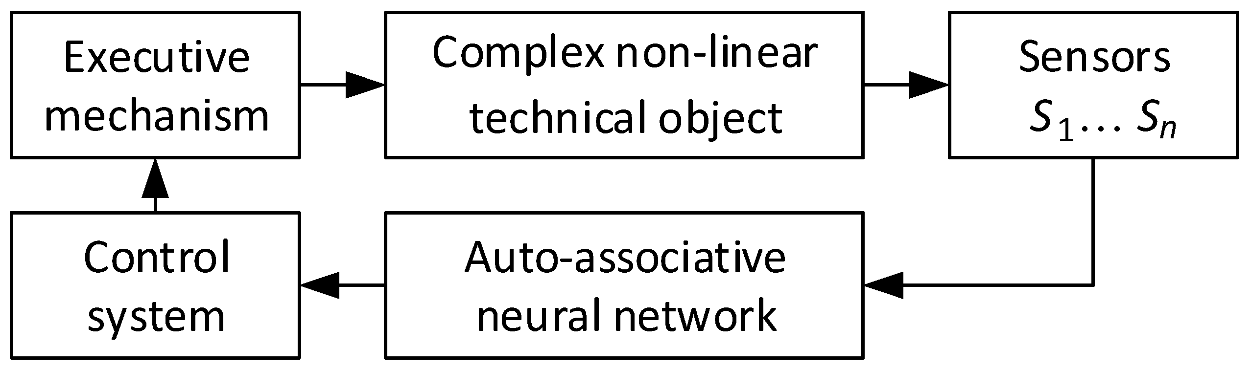
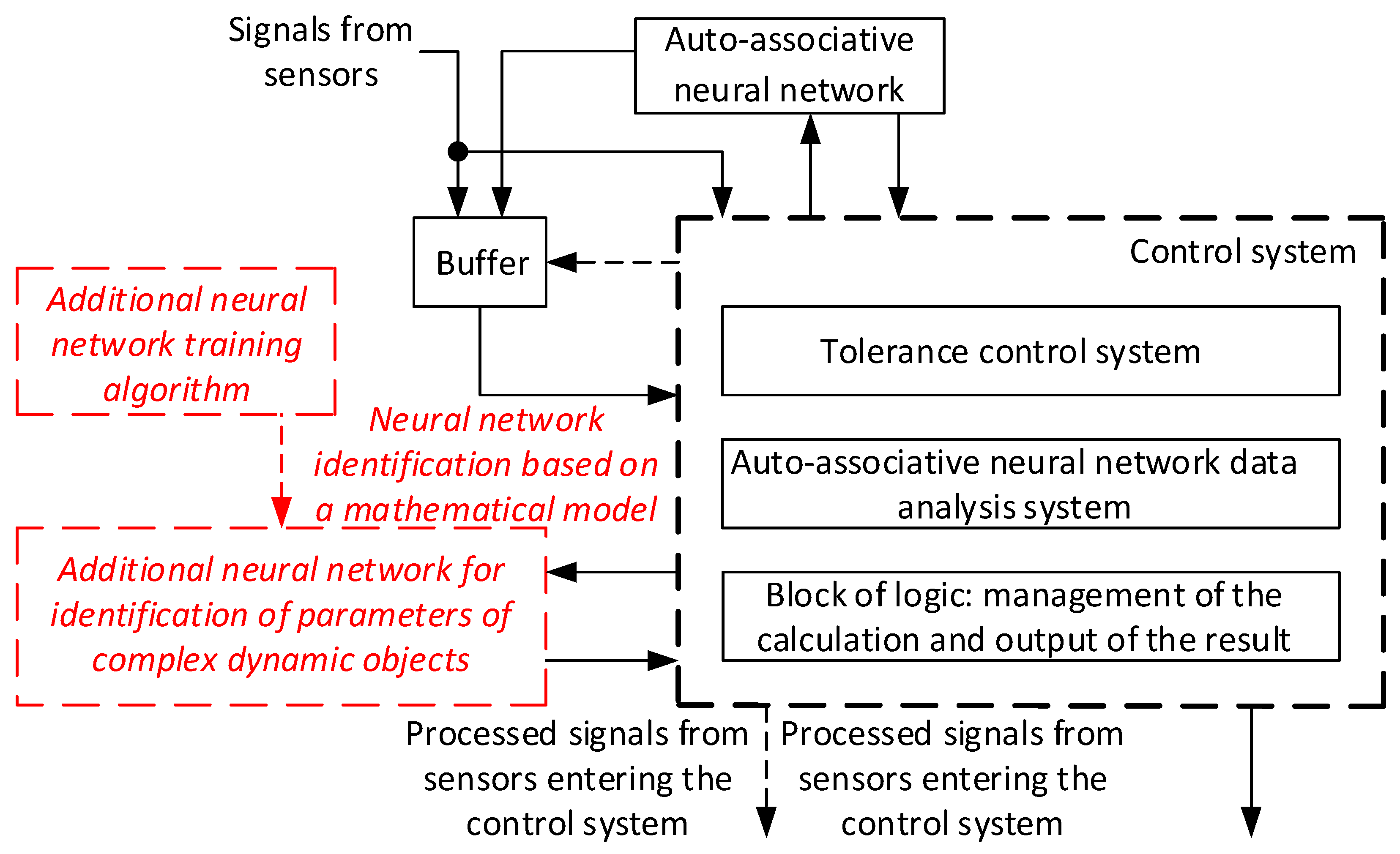
  • The functional diagram of the system for restoring lost information has been improved, which is based on an additional neural network to identify the complex dynamic object parameters, and significant accuracy and efficiency of the lost information restoration process in the event of complex dynamic object sensor failures are achieved. This is explained by a decrease in the maximum error values in restoring lost information, namely:
    -
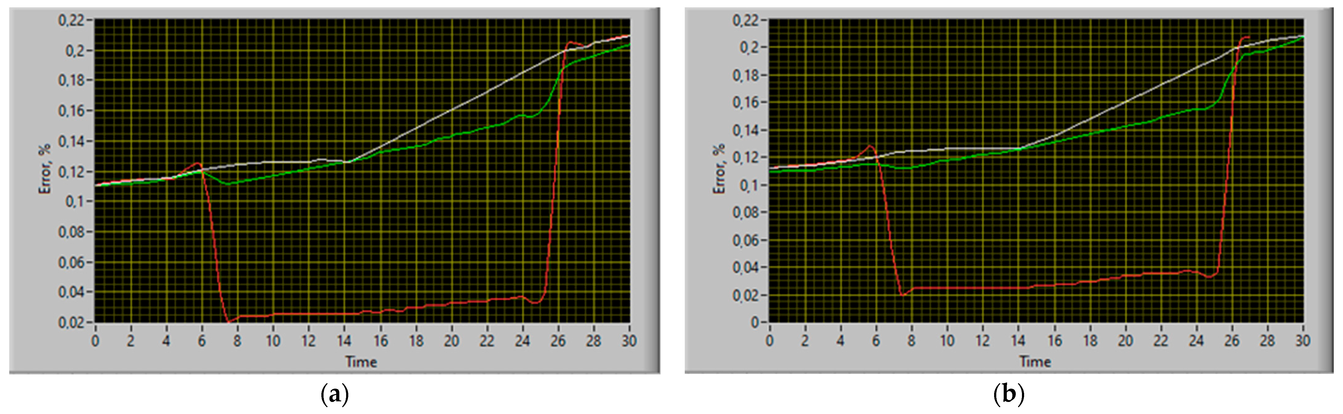
    A single sensor failure (break) example used for the TV3-117 turboshaft engine—it was established that the maximum error in restoring its parameters does not exceed 0.39%, while the maximum error in restoring its parameters using the basic functional diagram of the system for restoring lost information, developed by Zhernakov and Musluhov, is 0.42% [9,10,11], which is almost 10% more and can be critical during the complex dynamic object parameter identification, such as the TV3-117 turboshaft engine, under operating conditions;
    -
    A double (multiple) failure example used for the TV3-117 turboshaft engine sensors (breaks)—it was established that the maximum error in restoring its parameters does not exceed 0.50%, while the maximum error in restoring its parameters using the basic functional diagram of the system for restoring lost information, developed by Zhernakov and Musluhov, is 0.58% [9,10,11], which is almost 14% more and can be critical during the complex dynamic object parameter identification, such as the TV3-117 turboshaft engine, under operating conditions.
  • The auto-associative neural network (autoencoder) using effectiveness as part of the functional diagram for lost information restoration system of complex dynamic objects has been experimentally confirmed in comparison with other auto-associative neural network (autoencoder) models (convolutional autoencoder) and classical machine learning methods (linear regression, SVM, optimized SVM) according to these methods evaluation metrics such as precision, recall, F-measure, AUC, as well as training time:
    -
    When using an auto-associative neural network (autoencoder) with an improved basic algorithm for its training, the precision, recall, F-measure, and AUC metric values for normal data are 0.989, 0.987, 0.988, and 0.990, respectively, and for abnormal data—0.967, 0.967, 0.968, and 0.990, accordingly; when using a convolutional autoencoder, for normal data, they are 0.953, 0.949, 0.951, and 0.957, respectively, and for anomalous data—0.903, 0.902, 0.903, and 0.957, respectively, which is almost 3.33 to 6.81% more. At the same time, the training time for the auto-associative neural network (autoencoder) with an improved basic algorithm for its training was 5 min 43 s, and for the convolutional autoencoder—38 min 16 s, which indicates a reduction in training time and, as a consequence, improvement in lost information restoration by 6.69 times.
    -
    When using an auto-associative neural network (autoencoder) with an improved basic algorithm for its training, the precision, recall, F-measure, and AUC metric values for normal data are 0.989, 0.987, 0.988, and 0.990, respectively, and for abnormal data—0.967, 0.967, 0.968, and 0.990, accordingly; when applying a model based on linear regression, for normal data, they are 0.772, 0.622, 0.594, and 0.654, respectively, and for abnormal data—0.685, 0.522, 0.466, and 0.654, respectively, which is almost 21.94 to 51.86% more. At the same time, the training time for an auto-associative neural network (autoencoder) with an improved basic algorithm for its training was 5 min 43 s, and for a model based on linear regression—2 min 11 s. Although models based on linear regression train 2.62 times faster than auto-associative neural network models (autoencoder), their use in lost information restoration tasks for complex dynamic objects reduces accuracy by 21.94 to 51.86%.
    -
    When using an auto-associative neural network (autoencoder) with an improved basic algorithm for its training, the precision, recall, F-measure, and AUC metric values for normal data are 0.989, 0.987, 0.988, and 0.990, respectively, and for abnormal data—0.967, 0.967, 0.968, and 0.990, accordingly; when using a model based on the SVM, for normal data, they are 0.902, 0.903, 0.902, and 0.904, respectively, and for abnormal data—0.788, 0.781, 0.784, and 0.904, respectively, which is almost 8.51 to 19.23% more. At the same time, the training time for an auto-associative neural network (autoencoder) with an improved basic algorithm for its training was 5 min 43 s, and for a model based on the SVM—6 min 11 s, which indicates a reduction in training time and, as a consequence, improvement in restoring lost information by 1.08 times.
    -
    When using an auto-associative neural network (autoencoder) with an improved basic algorithm for its training, the precision, recall, F-measure, and AUC metric values for normal data are 0.989, 0.987, 0.988, and 0.990, respectively, and for abnormal data—0.967, 0.967, 0.968, and 0.990, accordingly; when using a model based on the optimized SVM, for normal data, they are 0.949, 0.943, 0.945, and 0.948, respectively, and for abnormal data—0.795, 0.798, 0.793, and 0.948, respectively, which is almost 4.04 to 18.08% more. At the same time, the training time of the auto-associative neural network (autoencoder) with an improved basic algorithm for its training was 5 min 43 s. The model based on the optimized SVM was 18 min 24 s, which indicates a reduction in training time and, as a consequence, improvement in lost information restoration by 3.22 times.

6. Conclusions

This work demonstrates a significant improvement in recovering lost information in the event of complex dynamic object sensor failures using an auto-associative neural network (autoencoder), providing restoration accuracy of more than 99%. An improved autoencoder training algorithm with regularization has been experimentally verified to reduce the model overfitting risk, and a new weight-updating hypothesis using gradient descent highlights this approach’s importance. The auto-associative neural network’s additional implementation to identify object parameters significantly increases the accuracy and efficiency of the lost information restoration process.

Author Contributions

Conceptualization, S.V. and V.V.; methodology, S.V.; software, V.V. and V.L.; validation, S.V., V.V. and V.L.; formal analysis, S.V.; investigation, M.N.; resources, S.V., R.Y. and V.V.; data curation, M.N.; writing—original draft preparation, S.V. and V.V.; writing—review and editing, M.N. and V.L.; visualization, V.V. and V.L.; supervision, S.V.; project administration, R.Y.; funding acquisition, M.N. All authors have read and agreed to the published version of the manuscript.

Funding

This research received no external funding.

Data Availability Statement

Data available upon request.

Acknowledgments

This research was supported by the Ministry of Internal Affairs of Ukraine as “Theoretical and applied aspects of the aviation sphere development” under project No. 0123U104884 and by the Ministry of Education and Science of Ukraine “Methods and means of identification of combat vehicles based on deep learning technologies for automated control of target distribution” under project No. 0124U000925.

Conflicts of Interest

The authors declare no conflicts of interest.

References

  1. Lutsenko, I.; Mykhailenko, O.; Dmytriieva, O.; Rudkovskyi, O.; Kukharenko, D.; Kolomits, H.; Kuzmenko, A. Development of a method for structural optimization of a neural network based on the criterion of resource utilization efficiency. East.-Eur. J. Enterp. Technol. 2019, 2, 57–65. [Google Scholar] [CrossRef]
  2. Pang, S.; Li, Q.; Ni, B. Improved nonlinear MPC for aircraft gas turbine engine based on semi-alternative optimization strategy. Aerosp. Sci. Technol. 2021, 118, 106983. [Google Scholar] [CrossRef]
  3. Kuzin, T.; Borovicka, T. Early Failure Detection for Predictive Maintenance of Sensor Parts. CEUR Workshop Proc. 2016, 1649, 123–130. Available online: https://ceur-ws.org/Vol-1649/123.pdf (accessed on 23 December 2023).
  4. Li, D.; Wang, Y.; Wang, J.; Wang, C.; Duan, Y. Recent advances in sensor fault diagnosis: A review. Sens. Actuators A Phys. 2020, 309, 111990. [Google Scholar] [CrossRef]
  5. Ntantis, E.L.; Botsaris, P. Diagnostic methods for an aircraft engine performance. J. Eng. Sci. Technol. 2015, 8, 64–72. [Google Scholar] [CrossRef]
  6. Krivosheev, I.; Rozhkov, K.; Simonov, N. Complex Diagnostic Index for Technical Condition Assessment for GTE. Procedia Eng. 2017, 206, 176–181. [Google Scholar] [CrossRef]
  7. Krukowski, M. Majority rule as a unique voting method in elections with multiple candidates. arXiv 2023, arXiv:2310.12983. Available online: https://arxiv.org/pdf/2310.12983.pdf (accessed on 29 December 2023).
  8. Shen, Y.; Khorasani, K. Hybrid multi-mode machine learning-based fault diagnosis strategies with application to aircraft gas turbine engines. Neural Netw. 2020, 130, 126–142. [Google Scholar] [CrossRef] [PubMed]
  9. Zhernakov, S.V.; Musluhov, I.I. Neurocomputer for recovering lost information from standard sensors of the on-board monitoring and diagnostic system. Neuroinformatics 2006, 3, 180–188. [Google Scholar]
  10. Zhernakov, S.V.; Musluhov, I.I. Parrying sensor failures in gas turbine engines using neural networks. Comput. Technol. New Inf. Technol 2003, 1, 35–41. [Google Scholar]
  11. Vasiliev, V.I.; Zhernakov, S.V.; Musluhov, I.I. Onboard algorithms for control of GTE parameters based on neural network technology. Bull. USATU 2009, 12, 61–74. [Google Scholar]
  12. Li, B.; Zhao, Y.-P.; Chen, Y.-B. Unilateral alignment transfer neural network for fault diagnosis of aircraft engine. Aerosp. Sci. Technol. 2021, 118, 107031. [Google Scholar] [CrossRef]
  13. Zocco, F.; McLoone, S. Recovery of linear components: Reduced complexity autoencoder designs. Eng. Appl. Artif. Intell. 2022, 109, 104663. [Google Scholar] [CrossRef]
  14. Gong, D.; Liu, L.; Le, V.; Saha, B.; Mansour, M.R.; Venkatesh, S.; van den Hengel, A. Memorizing Normality to Detect Anomaly: Memory-augmented Deep Autoencoder for Unsupervised Anomaly Detection. In Proceedings of the 2019 IEEE/CVF International Conference on Computer Vision (ICCV), Seoul, Republic of Korea, 27 October–2 November 2019; pp. 1705–1714. [Google Scholar] [CrossRef]
  15. Karpenko, D.; Dolgikh, S.; Prystavka, P.; Cholyshkina, O. Automated object recognition system based on convolutional autoencoder. In Proceedings of the 10th International Conference on Advanced Computer Information Technologies (ACIT-2020), Deggendorf, Germany, 16–18 September 2020. [Google Scholar] [CrossRef]
  16. Phan, P.H.; Nguyen, A.Q.; Quach, L.-D.; Tran, H.N. Robust Autonomous Driving Control using Auto-Encoder and End-to-End Deep Learning under Rainy Conditions. In Proceedings of the 2023 8th International Conference on Intelligent Information Technology, New York, NY, USA, 24–26 February 2023; pp. 271–278. [Google Scholar] [CrossRef]
  17. Campo, D.; Slavic, G.; Baydoun, M.; Marcenaro, L.; Regazzoni, C. Continual Learning of Predictive Models In Video Sequences Via Variational Autoencoders. In Proceedings of the 2020 IEEE International Conference on Image Processing (ICIP), Abu Dhabi, United Arab Emirates, 25–28 October 2020. [Google Scholar] [CrossRef]
  18. Fu, Y.; Yang, B.; Ye, O. Spatiotemporal Masked Autoencoder with Multi-Memory and Skip Connections for Video Anomaly Detection. Electronics 2024, 13, 353. [Google Scholar] [CrossRef]
  19. Nazarkevych, M.; Dmytruk, S.; Hrytsyk, V.; Vozna, O.; Kuza, A.; Shevchuk, O.; Sheketa, V.; Maslanych, I.; Voznyi, Y. Evaluation of the Effectiveness of Different Image Skeletonization Methods in Biometric Security Systems. Int. J. Sens. Wirel. Commun. Control. 2020, 11, 542–552. [Google Scholar] [CrossRef]
  20. Baranovskyi, D.; Bulakh, M.; Michajłyszyn, A.; Myamlin, S.; Muradian, L. Determination of the Risk of Failures of Locomotive Diesel Engines in Maintenance. Energies 2023, 16, 4995. [Google Scholar] [CrossRef]
  21. Baranovskyi, D.; Myamlin, S. The criterion of development of processes of the self organization of subsystems of the second level in tribosystems of diesel engine. Sci. Rep. 2023, 13, 5736. [Google Scholar] [CrossRef]
  22. Shi, H.; Shi, X.; Dogan, S. Speech Inpainting Based on Multi-Layer Long Short-Term Memory Networks. Future Internet 2024, 16, 63. [Google Scholar] [CrossRef]
  23. Dutta, R.; Kandath, H.; Jayavelu, S.; Xiaoli, L.; Sundaram, S.; Pack, D. A decentralized learning strategy to restore connectivity during multi-agent formation control. Neurocomputing 2023, 520, 33–45. [Google Scholar] [CrossRef]
  24. Ushakov, N.; Ushakov, V. Statistical analysis of rounded data: Recovering of information lost due to rounding. J. Korean Stat. Soc. 2017, 46, 426–437. [Google Scholar] [CrossRef]
  25. Lin, R.; Liu, S.; Jiang, J.; Li, S.; Li, C.; Jay Kuo, C.-C. Recovering sign bits of DCT coefficients in digital images as an optimization problem. J. Vis. Commun. Image Represent. 2024, 98, 104045. [Google Scholar] [CrossRef]
  26. Takada, T.; Hoogland, J.; van Lieshout, C.; Schuit, E.; Collins, G.S.; Moons, K.G.M.; Reitsma, J.B. Accuracy of approximations to recover incompletely reported logistic regression models depended on other available information. J. Clin. Epidemiol. 2022, 143, 81–90. [Google Scholar] [CrossRef]
  27. Shiroma, Y.; Kinoshita, Y.; Imoto, K.; Shiota, S.; Ono, N.; Kiya, H. Missing data recovery using autoencoder for multi-channel acoustic scene classification. In Proceedings of the 2022 30th European Signal Processing Conference (EUSIPCO), Belgrade, Serbia, 29 August–2 September 2022. [Google Scholar] [CrossRef]
  28. Manuel Lopez-Martin, M.; Carro, B.; Sanchez-Esguevillas, A.; Lloret, J. Conditional Variational Autoencoder for Prediction and Feature Recovery Applied to Intrusion Detection in IoT. Sensors 2017, 17, 1967. [Google Scholar] [CrossRef] [PubMed]
  29. Yu, X.; Li, H.; Zhang, Z.; Gan, C. The Optimally Designed Variational Autoencoder Networks for Clustering and Recovery of Incomplete Multimedia Data. Sensors 2019, 19, 809. [Google Scholar] [CrossRef] [PubMed]
  30. Abitbul, K.; Dar, Y. Recovery of Training Data from Overparameterized Autoencoders: An Inverse Problem Perspective. arXiv 2023, arXiv:2310.02897. Available online: https://arxiv.org/pdf/2310.02897.pdf (accessed on 10 February 2024). [CrossRef]
  31. Liu, Y.; Tan, X.; Bao, Y. Machine learning-assisted intelligent interpretation of distributed fiber optic sensor data for automated monitoring of pipeline corrosion. Measurement 2024, 226, 114190. [Google Scholar] [CrossRef]
  32. Casella, M.; Dolce, P.; Ponticorvo, M.; Marocco, D. Autoencoders as an alternative approach to Principal Component Analysis for dimensionality reduction. An application on simulated data from psychometric models. CEUR Workshop Proc. 2022, 3100. Available online: https://ceur-ws.org/Vol-3100/paper19.pdf (accessed on 15 February 2024).
  33. Casella, M.; Dolce, P.; Ponticorvo, M.; Marocco, D. From Principal Component Analysis to Autoencoders: A comparison on simulated data from psychometric models. In Proceedings of the 2022 IEEE International Conference on Metrology for Extended Reality, Artificial Intelligence and Neural Engineering (MetroXRAINE), Rome, Italy, 26–28 October 2022. [Google Scholar] [CrossRef]
  34. Shah, B.; Sarvajith, M.; Sankar, B.; Thennavarajan, S. Multi-Auto Associative Neural Network based sensor validation and estimation for aero-engine. In Proceedings of the 2013 IEEE AUTOTESTCON, Schaumburg, IL, USA, 16–19 September 2013. [Google Scholar] [CrossRef]
  35. Catana, R.M.; Dediu, G. Analytical Calculation Model of the TV3-117 Turboshaft Working Regimes Based on Experimental Data. Appl. Sci. 2023, 13, 10720. [Google Scholar] [CrossRef]
  36. Gebrehiwet, L.; Nigussei, Y.; Teklehaymanot, T. A Review-Differentiating TV2 and TV3 Series Turbo Shaft Engines. Int. J. Res. Publ. Rev. 2022, 3, 1822–1838. [Google Scholar] [CrossRef]
  37. Vladov, S.; Shmelov, Y.; Yakovliev, R.; Petchenko, M. Modified Neural Network Fault-Tolerant Closed Onboard Helicopters Turboshaft Engines Automatic Control System. CEUR Workshop Proc. 2023, 3387, 160–179. Available online: https://ceur-ws.org/Vol-3387/paper13.pdf (accessed on 24 February 2024).
  38. Vladov, S.; Yakovliev, R.; Hubachov, O.; Rud, J.; Stushchanskyi, Y. Neural Network Modeling of Helicopters Turboshaft Engines at Flight Modes Using an Approach Based on “Black Box” Models. CEUR Workshop Proc. 2024, 3624, 116–135. Available online: https://ceur-ws.org/Vol-3624/Paper_11.pdf (accessed on 24 February 2024).
  39. Vladov, S.; Yakovliev, R.; Bulakh, M.; Vysotska, V. Neural Network Approximation of Helicopter Turboshaft Engine Parameters for Improved Efficiency. Energies 2024, 17, 2233. [Google Scholar] [CrossRef]
  40. Corotto, F.S. Appendix C—The method attributed to Neyman and Pearson. In Wise Use of Null Hypothesis Tests; Academic Press: San Diego, CA, USA, 2023; pp. 179–188. [Google Scholar] [CrossRef]
  41. Motsnyi, F.V. Analysis of Nonparametric and Parametric Criteria for Statistical Hypotheses Testing. Chapter 1. Agreement Criteria of Pearson and Kolmogorov. Stat. Ukr. 2018, 83, 14–24. [Google Scholar] [CrossRef]
  42. Babichev, S.; Krejci, J.; Bicanek, J.; Lytvynenko, V. Gene expression sequences clustering based on the internal and external clustering quality criteria. In Proceedings of the 2017 12th International Scientific and Technical Conference on Computer Sciences and Information Technologies (CSIT), Lviv, Ukraine, 5–8 September 2017. [Google Scholar] [CrossRef]
  43. Hu, Z.; Kashyap, E.; Tyshchenko, O.K. GEOCLUS: A Fuzzy-Based Learning Algorithm for Clustering Expression Datasets. Lect. Notes Data Eng. Commun. Technol. 2022, 134, 337–349. [Google Scholar] [CrossRef]
  44. Andresini, G.; Appice, A.; Malerba, D. Autoencoder-based deep metric learning for network intrusion detection. Inf. Sci. 2021, 569, 706–727. [Google Scholar] [CrossRef]
  45. Gornyi, B.E.; Ryjov, A.P.; Strogalov, A.S.; Zhuravlev, A.D.; Khusaenov, A.A.; Shergin, I.A.; Feshchenko, D.A.; Abdullaev, A.M.; Kontsevaya, A.V. The adverse clinical outcome risk assessment by in-depth data analysis methods. Intell. Syst. Theory Appl. 2021, 25, 23–45. [Google Scholar]
  46. Khusaenov, A.A. Autoassociative neural networks in a classification problem with truncated dataset. Intell. Syst. Theory Appl. 2022, 26, 33–41. [Google Scholar]
  47. Dong, X.; Bai, Y.-L.; Wan, W.-D. Kernel functions embed into the autoencoder to identify the sparse models of nonlinear dynamics. Commun. Nonlinear Sci. Numer. Simul. 2024, 131, 107869. [Google Scholar] [CrossRef]
  48. Kanishima, Y.; Sudo, T.; Yanagihashi, H. Autoencoder with Adaptive Loss Function for Supervised Anomaly Detection. Procedia Comput. Sci. 2022, 207, 563–572. [Google Scholar] [CrossRef]
  49. Impraimakis, M. A Kullback–Leibler divergence method for input–system–state identification. J. Sound Vib. 2024, 569, 117965. [Google Scholar] [CrossRef]
  50. Vladov, S.I.; Doludarieva, Y.S.; Siora, A.S.; Ponomarenko, A.V.; Yanitskyi, A.A. Neural network computer for recovering lost information from standard sensors of the on-board system for control and diagnosing of TV3-117 aircraft engine. Innov. Technol. Sci. Solut. Ind. 2020, 4, 147–154. [Google Scholar] [CrossRef]
  51. Safronov, D.A.; Kazer, Y.D.; Zaytsev, K.S. Anomaly detection with autoencoders. Int. J. Open Inf. Technol. 2022, 10, 39–45. [Google Scholar]
  52. Gus’kov, S.Y.; Lyovin, V.V. Confidence interval estimation for quality factors of binary classifiers–ROC curves, AUC for small samples. Eng. J. Sci. Innov. 2015, 3, 1–15. Available online: http://engjournal.ru/catalog/mesc/idme/1376.html (accessed on 10 March 2024).
Figure 1. The proposed auto-associative neural network architecture diagram for lost information restoration in the TV3-117 turboshaft engine sensor failure event [9,10,11,32,33].
Asi 07 00053 g001
Figure 2. An auto-associative neural network training error dependence diagram example of the neurons’ number in the hidden layer [9,10,11].
Asi 07 00053 g002
Figure 3. Functional information restoration diagram based on auto-associative neural network [9,10,11].
Asi 07 00053 g003
Figure 4. Functional control diagram of a complex nonlinear technical object based on an auto-associative neural network ([9]).
Asi 07 00053 g004
Figure 5. Clustering outcomes: (a) original experimental data set (I…VIII—classes); (b) training data set (authors’ research, published in [37,38,39,40]).
Asi 07 00053 g005
Figure 6. The main component diagram for the set Xn on a two-dimensional plane where black points are F2(V) and white points are X: (a) Experiment I; (b) Experiment II; (c) Experiment III; (d) Experiment IV; (e) Experiment V; (f) Experiment VI (authors’ research, based on [45]).
Asi 07 00053 g006
Figure 7. The feature set diagram for one of the two-dimensional planes: (b) errors set for the plane (a) where the black points are Y0 and the white points are Y1 (authors’ research, based on [45]).
Asi 07 00053 g007
Figure 8. Classification diagram on the error plane where the black points are Y0 and the white points are Y1 (authors’ research, based on [45]).
Asi 07 00053 g008
Figure 9. The auto-associative neural network training feature diagram: (a) permissible generalizing ability; (b) retraining [45].
Asi 07 00053 g009
Figure 10. The loss function dynamics diagram at the model training and validation stages.
Asi 07 00053 g010
Figure 11. Kullback–Leibler divergence diagram.
Asi 07 00053 g011
Figure 12. Virtual installation in the LabVIEW software package, simulating a system with three sensors.
Asi 07 00053 g012
Figure 13. The lost information restoration result diagrams: (a) in the failure case of one of the regular sensors; (b) in a single failure case of sensors (their breaks) (authors’ research, based on [9,10,11,50]).
Asi 07 00053 g013
Figure 14. Improved functional diagram for the lost information restoring system (authors’ research, based on [9,10,11,50]).
Asi 07 00053 g014
Figure 15. The auto-associative neural network lost information restoration from the gas temperature sensor in the compressor turbine front for the TV3-117 turboshaft engine in the sensor failure event (authors’ research, based on [9,10,11,50]).
Asi 07 00053 g015
Table 1. Training sample fragment (authors’ research, published in [37,38,39]).
NumberFree Turbine Rotor SpeedGas Generator
Rotor r.p.m
Gas Temperature in the Compressor Turbine FrontFuel
Consumption
10.9430.9290.9320.952
580.9850.9830.8990.931
1440.9820.9800.8760.925
2560.9810.9730.9530.960
Table 2. Auto-associative neural network training parameters (authors’ research based on [44]).
EncoderDecoderEpochBatch SizeTraining DataTest DataOptimizer
ReLUSigmoid2002505 × 10−41 × 10−4Adam
Table 3. Auto-associative neural network information restoration results in sensor failure cases.
Auto-Associative Neural Network StructureTV3-117 Turboshaft Engine Parameter Restoration Error,%
GTnTCnFT T G
4–3–4 as part of the proposed improved functional diagram (Figure 14)0.310.280.190.31
5–4–5 as part of a basic functional diagram developed by Zhernakov and Musluhov [9,10,11]0.330.310.240.42
Table 4. Auto-associative neural network information restoration results in double (multiple) sensor failure cases.
Auto-Associative Neural Network StructureTV3-117 Turboshaft Engine Parameter Restoration Error,%
GTnTCnFT T G *
4–3–4 as the proposed improved functional diagram part (Figure 14)0.420.390.400.43
5–4–5 as a basic functional diagram part developed by Zhernakov and Musluhov [9,10,11]0.560.450.440.58
Table 5. A comparative analysis results of the proposed auto-associative neural network with a convolutional autoencoder and classical machine learning methods (authors’ research, based on [52]).
Algorithm for Restoring Lost InformationData
Types
Metrics for Evaluating MethodsTraining
Time
PrecisionRecallF-MeasureAUC
Proposed ANNNormal0.9890.9870.9880.9905 min 43 s
Abnormal0.9670.9670.968
Convolutional autoencoderNormal0.9530.9490.9510.95738 min 16 s
Abnormal0.9020.9030.902
Linear regressionNormal0.7720.6220.5940.6542 min 11 s
Abnormal0.6850.5220.466
SVMNormal0.9020.9030.9020.9046 min 11 s
Abnormal0.7880.7810.784
SVM (optimized)Normal0.9490.9430.9450.94818 min 24 s
Abnormal0.7950.7980.793
Table 6. A comparative analysis results of the proposed auto-associative network with a famous auto-associative network in the lost information restoring method, developed by Zhernakov and Musluhov in [9,10,11].
CriterionProposed MethodThe Closest Analog [9,10,11]Proposed Method Advantages
ANN structure choiceANN structure choice is carried out according to a decrease in the neuron number in the output layer by one.ANN structure choice is carried out based on the minimum error in reconstructing ANN information from the neurons’ number in the “shaft”.A simpler criterion for determining the ANN structure without losing its training accuracy (see metrics in Table 5).
ANS training methodModified ANN training method—gradient descent method with regularization.Traditional ANS training method—gradient descent method.The model overtraining risk reducing, with its strong adaptation to training data and the ability loss to generalize new data (see the loss function diagram, the maximum value of which does not exceed 2.5%, Figure 10)
Restoring lost informationThe maximum error in restoring lost information does not exceed 0.50% (see Table 4) in the TV3-117 TE sensor double (multiple) failure situations.The maximum error in restoring lost information does not exceed 0.58% (see Table 4) in the TV3-117 TE sensor double (multiple) failure situations.The lost information restoration accuracy increasing by 10 to 14% is of key importance when operating complex dynamic objects such as the TV3-117 TE in helicopter flight mode.
AccuracyThe lost ANN information restoration task solving accuracy on the test data set is 0.988 (98.8%).The lost ANN information restoration task solving accuracy on the test data set is 0.901 (90.1%).The lost ANN information restoration task solving accuracy increase on a test data set by 8.8% is critical when operating complex dynamic objects such as the TV3-117 TE in helicopter flight mode.
Training rateThe ANN training time using the proposed method of training was 5 min 43 s–343 s (AMD Ryzen 5 5600 processor, 32 KB third-level cache, Zen 3 architecture, 6 cores, 12 threads, 3.5 GHz, RAM—32 GB DDR-4).The ANN training time using the traditional method of training was 5 min 34 s–334 s (AMD Ryzen 5 5600 processor, 32 KB third-level cache, Zen 3 architecture, 6 cores, 12 threads, 3.5 GHz, RAM—32 GB DDR-4).During the ANN training using the proposed method, the speed practically does not decrease compared with the classical method of training (the decrease is by 9 s, which is insignificant), while the regularization introduction into the classical method of training reduces the risk of overtraining the model.
Generalization abilityThe determination coefficient was 0.996.The determination coefficient was 0.850.An increase in the determination coefficient by 14.7% indicates a 14.7% increase in the ANN efficiency to work on new data that it did not see during training.
Resource efficiencyTesting was carried out on an AMD Ryzen 5 5600 processor, 32 KB L3 cache, Zen 3 architecture, 6 cores, 12 threads, 3.5 GHz, 32 GB DDR-4 RAM, with an efficiency metric of 0.00288.Testing was carried out on an AMD Ryzen 5 5600 processor, 32 KB L3 cache, Zen 3 architecture, 6 cores, 12 threads, 3.5 GHz, 32 GB DDR-4 RAM, with an efficiency metric of 0.00270.The ANN proposed in this work demonstrates a 6.25% accuracy compared with [9,10,11] by the resources expended, which can be significant when operating complex dynamic objects such as the TV3-117 TE in helicopter flight mode.
RobustnessThe average deviation was 0.00524.The average deviation was 0.01148.A decrease in the average deviation by 45.6% indicates that the ANN proposed in this work is almost two times more robust compared with [9,10,11], which indicates the possibility of maintaining high accuracy on different data sets or under different conditions.
Table 7. Indicators of calculation result accuracy for the proposed auto-associative network with a famous network in the restoration of lost information method, developed by Zhernakov and Musluhov in [9,10,11], with a training sample of 256 elements divided into 8 subsamples of 32 elements each.
Subsample Number12345678 A c c ¯
Proposed Method (ANN 1)0.9910.9820.9840.9810.9850.9940.9950.9920.988
The closest Analog [9,10,11] (ANN 2)0.9140.9130.9060.8890.8930.8880.9150.8890.901
Disclaimer/Publisher’s Note: The statements, opinions and data contained in all publications are solely those of the individual author(s) and contributor(s) and not of MDPI and/or the editor(s). MDPI and/or the editor(s) disclaim responsibility for any injury to people or property resulting from any ideas, methods, instructions or products referred to in the content.

