Switched Observer Design for a Class of Non-Linear Systems

Abstract

This paper is concerned with the switched observer design for a class of systems subject to locally Lipschitz non-linearities. By performing a suitable description of the estimation error dynamics into a linear parameter varying (LPV) system representation, sufficient conditions for the existence of a switching output injection gain are proposed such that the asymptotic stability of the estimation error is guaranteed. These conditions can be conveniently expressed by means of linear matrix inequalities (LMIs), which are easily computationally tractable. A numerical example is provided to show the favorable performance achieved by the proposed observer, which can be applied to a large class of non-linear systems.

1. Introduction

State observer design for continuous-time dynamical systems is still a topic of significant research interest in control engineering. In several applications, a reliable state estimation of the unmeasurable state variables is required, particularly, when they are employed for either monitoring or model-based control design purposes. The state observer design problem is substantially more challenging when dealing with non-linear dynamical systems, which have attracted a lot of interest in control and systems literature for several decades. As a result, numerous results addressing the design of state observers and filters for non-linear systems were proposed, having different levels of conservatism; see, e.g., [1,2,3,4,5] and the references therein.

Throughout recent decades, significant attention arose for the class of Lipschitz non-linear control systems that have been extensively studied in the literature. As we know, most physical systems models satisfy the Lipschitz condition, at least locally. Specifically, in the context of state estimation, the so-called Lipschitz non-linear observer has been thoroughly investigated in the literature (see, for instance [6,7,8,9,10]). The limitation of all these approaches is that the synthesis conditions usually become unfeasible for systems with large Lipschitz constants. Some relatively recent results offer a proper reformulation of non-linear dynamical systems by the application of mathematical principles that, for the general class of Lipschitz systems, directly lead to the linear parameter varying (LPV) approach and, hence, to less restrictive synthesis conditions [11,12].

On the other hand, many stabilization techniques on the field of dynamical systems use the concept of switching structure to compensate for system variations and fluctuations caused by uncertainties and perturbations. Switching stabilization methods have been proven to be successful against parameter uncertainties [13,14,15,16,17]. The  general approach consists of constructing a state-dependent switching strategy and adaptive stabilization control law consisting of a set of feedback gains, each of which is selected at certain time instants according to the switching strategy, which is derived from the Lyapunov stability theory.

Most of the previously published LMI-based observer design methods for non-linear systems consider a single observer gain matrix, whereas a set of observer gain matrices in a switched scheme of implementation are also needed in order to achieve and/or increase the feasibility range of the design parameters as well as to improve the state estimation performance. A recent result of importance develops a hybrid switched-gain observer for non-monotonic non-linear systems [18] and whose application has been depicted in [19,20,21,22]. Furthermore, the hybrid switched-gain observer design has been extended for systems with disturbances in both the state dynamics and in the output measurements, and its $H_{\infty }$ performance has been investigated  [23]. In regard to non-linear systems with asynchronous switching, some recent results involve observer-based control for time-delayed non-linear systems [24] and robust state and sensor fault estimation [25,26,27].

Although the results from the literature above show a considerable advancement in the development of workable switched observer design methods, most of them consider asynchronous switching schemes of implementation for systems that incorporate switching in their dynamics, which limits their applicability to practical non-linear systems where switching may be included to take advantage of the previously mentioned benefits of this scheme. In particular, this study considers an LPV representation of the non-linear state estimation error dynamics, which is inferred directly from the general Lipschitz condition and the application of the differential mean value theorem (DMVT), requiring no extra assumptions on system non-linearities. The convergence and performance analysis is studied in the framework of a semi-definite programming (SDP) problem in terms of LMI conditions which contain more degrees of freedom than the classical approach of invariant structure observer. It is also shown that the proposed method encompasses the switching strategy design and a set of observer gains, which ensure the local exponential stability of the estimation error dynamics while estimating a set of admissible initial conditions. Finally, we extend the observer design methodology to cope with energy bounded exogenous disturbances into an $H_{\infty }$ setting. Analytical and simulation comparisons are also provided to demonstrate the superiority of the new LMI design methodology compared to previous results. In this context, the contribution of this work can be summarized as follows:

• A non-linear Luenberger-like switched observer with a guaranteed decay rate and $H_{\infty }$ cost for the estimation of error dynamics is designed in terms of LMI constraints, considering a class of non-linear systems locally satisfying a Lipschitz condition.

The remainder of this paper is organized as follows. Section 2 describes the system dynamics along with some preliminary assumptions introduced in order to ensure the well-posedness of the LPV formulation of the state estimation error dynamics. Section 2.1 proposes LMI design conditions considering the representative LPV system, which guarantees both the local exponential stability of the closed loop system with prescribed decay rate and an $H_{\infty }$ guaranteed cost. Section 4 applies the proposed methodology to a representative system, and Section 5 draws concluding remarks and points out some possible research lines.

The following notation and definitions will be used throughout the paper:

• ${\mathbb{N}}_{+}$, $\mathbb{R}$, ${\mathbb{R}}^n$, and ${\mathbb{R}}^{n_x\times n_y}$ represent, respectively, the set of non-negative integer numbers, real numbers, n-dimensional real vectors, and of $n\times m$ real matrices;
• ${\mathbb{S}}^n\subset {\mathbb{R}}^{n\times n}$ represents the subspace of square symmetric matrices;
• For $A\in {\mathbb{R}}^{r\times m}$, $A^T$ denotes the transpose of A;
• For $P\in {\mathbb{S}}^n$, $P>0(P<0)$ means that P is positive definite (negative definite), and ${\mathrm{H}}_{\mathrm{e}}\left\{P\right\}=P+P^T$ represents the Hermitian operator applied to P;
• The set $\mathrm{Co}(x,\widehat{x})=\{\lambda x+(1-\lambda )\widehat{x}:\lambda \in [0,1]\}$ is the convex hull of $\{x,\widehat{x}\}$;
• $e_s\left(i\right)=\underset{s\mathrm{components}}{\underbrace{{\{0,...,0,\stackrel{i\mathrm{th}}{\overbrace{1}},0,...,0\}}^T}}\in {\mathbb{R}}^s$ is a vector of the canonical basis of ${\mathbb{R}}^s$;
• The set of all vectors $\lambda ={[{\lambda }_1,...,{\lambda }_N]}^T$, such that ${\lambda }_i\ge 0$, $i\in \{1,...,N\}$ and ${\lambda }_1+...+{\lambda }_N=1$ is designated by ${\Lambda }_N$;
• The convex combination of a set of matrices $Q_1,...,Q_N\in {\mathbb{R}}^{n\times m}$ is denoted by

  $$Q_{\lambda }=\sum _{i=1}^N{\lambda }_i{Q}_i,$$

  where $\lambda \in {\Lambda }_N$;
• The subset of Metzler matrices denoted $\mathcal{M}$ consists of all matrices $\Pi \in {\mathbb{R}}^{n\times n}$ with elements ${\pi }_{ji}$ such that ${\pi }_{ji}\ge 0\forall i\ne j$ and

  $$\sum _{j=1}^{n_p}{\pi }_{ji}=0,i,j\in \{1,...,n_p\};$$
• $\parallel ·\parallel$ is the Euclidean norm in ${\mathbb{R}}^n$, for every $n\in {\mathbb{N}}_{+}$;
• The set of trajectories $\zeta \left(t\right)\in {\mathbb{R}}^n$ with finite energy, i.e.,  ${\int }_0^{\infty }{\zeta }^T\left(t\right)\zeta \left(t\right)dt<\infty$, is denoted by ${\mathcal{L}}_2^n$.

Instrumental Tools. The following statements are instrumental for deriving the main theoretical results of this paper.

Lemma 1

(Differential mean value theorem [28]). Let $f:{\mathbb{R}}^{n_x}\to {\mathbb{R}}^{n_f}$. Let $x,\widehat{x}\in {\mathbb{R}}^{n_x}$. We assume that f is a differentiable function on $\mathrm{Co}(x,\widehat{x})$. Then, there are constant vectors ${\breve{x}}_1,...{\breve{x}}_{n_f}\in Co(x,\widehat{x})$, ${\breve{x}}_i\ne x$, ${\breve{x}}_i\ne \widehat{x}$ for $i=1,...,n_f$ such that:

$$f\left(x\right)-f\left(\widehat{x}\right)=\left(\sum _{i=1}^{i=n_f}\sum _{j=1}^{j=n_x}{e}_{n_f}\left(i\right)e_{n_x}{\left(j\right)}^T{\displaystyle \frac{\partial f_i}{\partial x_j}}\left({\breve{x}}_i\right)\right)(x-\widehat{x}).$$

Lemma 2

([11]). Considering the function $f(·):{\mathbb{R}}^{n_x}\to {\mathbb{R}}^{n_f}$, the two following statements are equivalent

• $f(·):{\mathbb{R}}^{n_x}\to {\mathbb{R}}^{n_f}$ is locally Lipschitz continuous in x, i.e., there exists a constant scalar $L_f$ such that

  $$\parallel f\left(x\right)-f\left(\widehat{x}\right)\parallel \le L_f\parallel (x-\widehat{x})\parallel$$

  (1)
  holds for all $x,\widehat{x}\in \mathcal{X}\subset {\mathbb{R}}^{n_x}$.
• for all $i,j=1,\cdots ,n$ there exist functions

  $$h_{ij}:{\mathbb{R}}^{n_x}\to \mathbb{R}$$
  and constants ${\overline{h}}_{ij}$ and ${\underline{h}}_{ij}$, such that $\forall x,\widehat{x}\in \mathcal{X}\subset {\mathbb{R}}^{n_x}$,

  $$f\left(x\right)-f\left(\widehat{x}\right)=\sum _{i=1}^{i=n_x}\sum _{j=1}^{j=n_x}{e}_{n_f}\left(i\right)e_{n_x}{\left(j\right)}^T{h}_{ij}(x-\widehat{x})$$
  and

  $${\underline{h}}_{ij}\le h_{ij}\le {\overline{h}}_{ij}.$$

Lemma 3

([29]). For a function

$$V\left(x\left(t\right)\right)=\underset{i\in 1,...,n_p}{min}{x}^T\left(t\right)P_{i}x\left(t\right),P_i\in {\mathbb{S}}^{n_x}$$

where $x\left(t\right)\in {\mathbb{R}}^{n_x}$ is a generic trajectory of the linear system $\dot{x}\left(t\right)=Ax\left(t\right)$, for all $t\ge 0$. For $h\to 0^{+}$, then $x(t+h)=x\left(t\right)+h\dot{x}\left(t\right)=x\left(t\right)+hAx\left(t\right)$ and hence the right-hand Dini derivative is defined as

$$D^{+}V(x\left(t\right),Ax\left(t\right))=\underset{h\to 0^{+}}{lim}{\displaystyle \frac{V\left(x\right(t)+hAx(t\left)\right)-V\left(x\right(t\left)\right)}{h}}$$

and applying Danskin’s Theorem [30], we obtain

$$\begin{array}{c}\hfill D^{+}V(x\left(t\right),Ax\left(t\right))=\underset{i\in 1,...,n_p}{\min }{x}^T\left(t\right)\left(A^T{P}_i+P_{i}A\right)x\left(t\right).\end{array}$$

2. System and Observer Description

Consider the following class of systems with Lipschitz non-linearity.

$$\begin{array}{cc}\hfill \dot{x}\left(t\right)& =Ax\left(t\right)+B_{f}f\left(x\left(t\right)\right)+g(y\left(t\right),u\left(t\right))+B_{d}d\left(t\right)\hfill \\ \hfill y\left(t\right)& =Cx\left(t\right)\hfill \end{array}$$

(2)

where $x\left(t\right)\in \mathcal{X}\subset {\mathbb{R}}^{n_x}$, with $\mathcal{X}$ being a compact domain, is the state vector, $u\left(t\right)\in {\mathbb{R}}^{n_u}$ is the input vector, $y\left(t\right)\in {\mathbb{R}}^{n_y}$ is the output measurement vector, and $d\in {\mathcal{L}}_2^{n_d}$ is an exogenous disturbance vector. The known functions $f:{\mathbb{R}}^{n_x}\to {\mathbb{R}}^{n_f}$, $g:{\mathbb{R}}^{n_y}\times {\mathbb{R}}^{n_u}\to {\mathbb{R}}^{n_x}$ are locally Lipschitz on the domain of interest. The matrices $A\in {\mathbb{R}}^{n_x\times n_x}$, $B_f\in {\mathbb{R}}^{n_x\times n_f}$, $B_d\in {\mathbb{R}}^{n_x\times n_d}$, and $C\in {\mathbb{R}}^{n_y\times n_x}$ are known constant matrices of appropriate dimensions. The initial condition is $x\left(0\right)=x_0\in {\mathbb{R}}^{n_x}$.

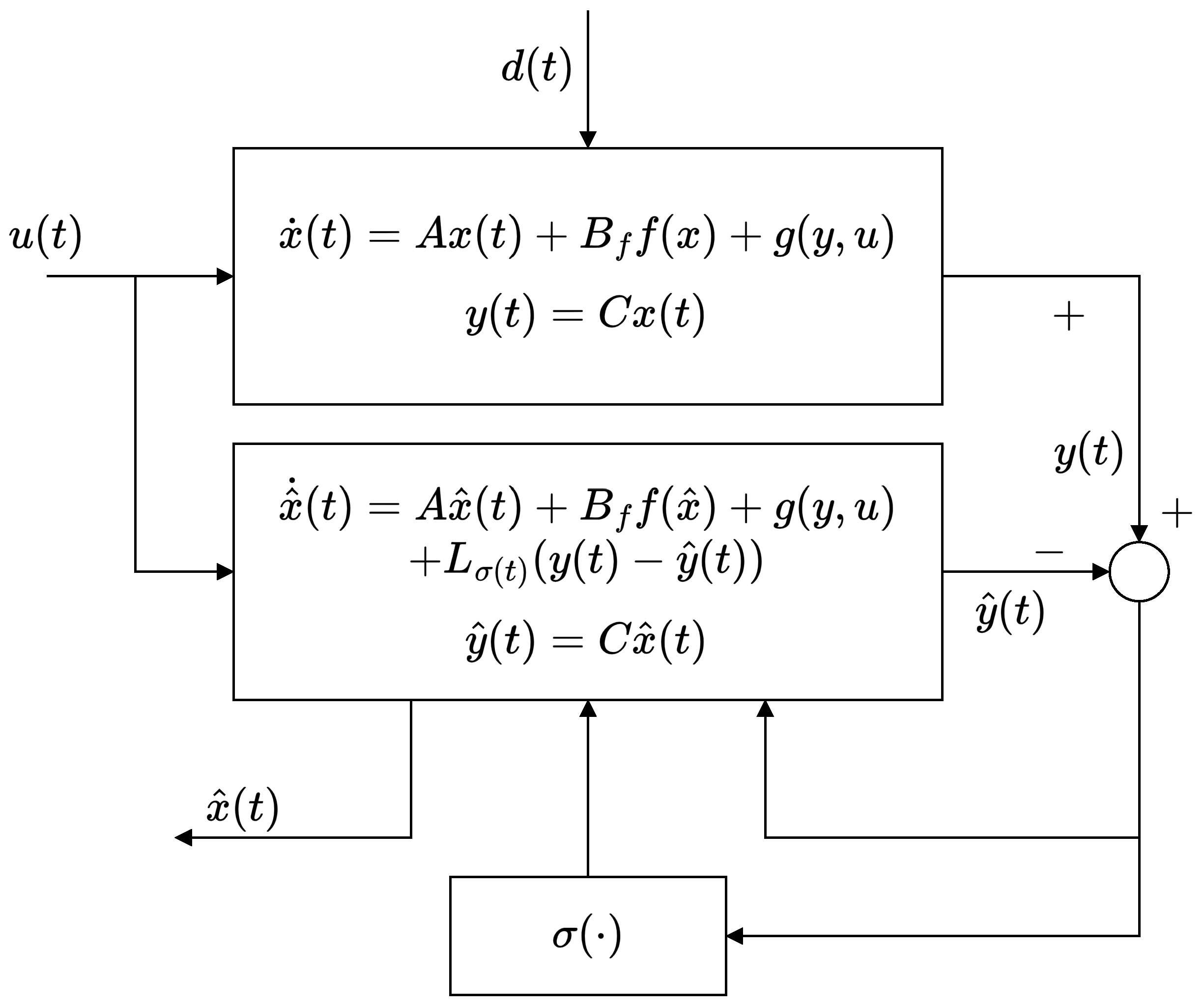
2.1. Switched Luenberger-like Observer

The following extended Luenberger-like observer is proposed to estimate the state vector $x\left(t\right)$:

$$\begin{array}{cc}\hfill \dot{\widehat{x}}\left(t\right)& =A\widehat{x}\left(t\right)+B_{f}f\left(\widehat{x}\left(t\right)\right)+g(y\left(t\right),u\left(t\right))+L_{\sigma \left(t\right)}(\widehat{y}\left(t\right)-y\left(t\right))\hfill \\ \hfill \widehat{y}\left(t\right)& =C\widehat{x}\left(t\right)\hfill \end{array}$$

(3)

where $\widehat{x}\left(t\right)\in {\mathbb{R}}^{n_x}$ is the estimated state and $L_{\sigma \left(t\right)}\in {\mathbb{R}}^{n_x\times n_y}$ is a switched output injection gain with $\sigma :{\mathbb{R}}^{n_y}\to \mathbb{N}$ as a switching rule to be designed. Now, let

$$\tilde{x}\left(t\right)=x\left(t\right)-\widehat{x}\left(t\right)$$

(4)

be the state estimation error and $\tilde{\mathcal{X}}$ be the set induced by

$$\tilde{\mathcal{X}}=\left\{\tilde{x}\in {\mathbb{R}}^{n_x}:\tilde{x}=x-\widehat{x},x,\widehat{x}\in \mathcal{X}\right\}.$$

Then, the estimation error dynamics is given by

$$\dot{\tilde{x}}\left(t\right)=A\tilde{x}\left(t\right)+B_f(f\left(x\left(t\right)\right)-f\left(\widehat{x}\left(t\right)\right))+L_{\sigma \left(t\right)}(\widehat{y}\left(t\right)-y\left(t\right))+B_{d}d\left(t\right)$$

(5)

where $\tilde{x}\in \tilde{\mathcal{X}}$. The switched observation problem consists in finding a gain $L_{\sigma \left(t\right)}$ and the corresponding switching rule $\sigma \left(y\right(t\left)\right)$ to ensure the stability of the estimation error dynamics (5).

2.2. LPV Formulation

Notice from the DMVT, there exists an $\breve{x}\in Co(x,\widehat{x})$ such that:

$$f\left(x\right)-f\left(\widehat{x}\right)=\left(\sum _{i=1}^{i=n_f}\sum _{j=1}^{j=n_x}{e}_{n_f}\left(i\right)e_{n_x}{\left(j\right)}^T{\displaystyle \frac{\partial f_i}{\partial x_j}}\left(\breve{x}\right)\right)(x-\widehat{x}).$$

Hence, using the notations

$$\begin{array}{cc}\hfill h_{ij}\left(t\right)& ={\displaystyle \frac{\partial f_i}{\partial x_j}}\left(\breve{x}\left(t\right)\right)\hfill \\ \hfill h\left(t\right)& =(h_{11}\left(t\right),...,h_{n_f{n}_x}\left(t\right))\hfill \end{array}$$

(6)

we may define

$$A\left(h\left(t\right)\right)=A+\sum _{i,j=1}^{n_f,n_x}{h}_{ij}\left(t\right)B_f{e}_{n_f}\left(i\right)e_{n_x}{\left(j\right)}^T$$

(7)

which casts the observer error dynamics in (5) as follows:

$$\dot{\tilde{x}}\left(t\right)=(A\left(h\left(t\right)\right)+L_{\sigma \left(t\right)}C)\tilde{x}\left(t\right)+B_{d}d\left(t\right).$$

(8)

Indeed, this representation allows us to have a more appropriate and flexible handling of the non-linearities in consideration while still making use of all of its time-varying properties according to the so called LPV formulation [31]. In light of this, and using the results presented in Lemma 2 for locally Lipschitz non-linear functions, the functions $h_{ij}$ in (7) are bounded according to

$${\overline{h}}_{ij}<h_{ij}\left(t\right)<{\underline{h}}_{ij},\forall t\ge 0$$

suggesting that the parameter $h\left(t\right)$ evolves in a bounded domain $\mathcal{H}$, of which its $n_p\le 2^{n_x{n}_f}$ vertices are defined by:

$${\mathcal{V}}_{\mathcal{H}}=\left\{(h_{11},...,h_{n_f{n}_x}):h_{ij}\in \left\{{\underline{h}}_{ij},{\overline{h}}_{ij}\right\}\right\}.$$

(9)

At this stage, we may even describe the estimation error dynamics in (8) as an uncertain-switched polytopic linear system

$$\dot{\tilde{x}}\left(t\right)=(A(\alpha \left(h\left(t\right)\right)+L_{\sigma \left(t\right)}C)\tilde{x}\left(t\right)+B_{d}d\left(t\right)$$

(10)

with

$$A\left(\alpha \left(h\left(t\right)\right)\right)=\sum _{j=1}^{n_p}{\alpha }_j\left(t\right)A_j$$

(11)

and the matrices $A_j,j=1,...,n_p$ are constructed by taking all elements of the set ${\mathcal{V}}_{\mathcal{H}}$ defined in (9) and

$$\begin{array}{cc}\hfill & \alpha \left(t\right)\in \Lambda =\hfill \\ \hfill & \left\{{[{\alpha }_1,...,{\alpha }_{n_p}]}^T\in {\mathbb{R}}^{n_p}:\sum _{j=1}^{n_p}{\alpha }_j=1,{\alpha }_j\ge 0\right\}.\hfill \end{array}$$

(12)

This description is the foundation of the switching design approach put forward in this work, which aims to improve the estimation performance in addition to reducing the conservatism of the stabilizing conditions, particularly in cases when the range of the time variant parameters is large [32].

2.3. Minimum-Type Switching Rule

Based on the results of [29], the minimum-type switching strategy is proposed

$$\sigma \left(t\right)=\underset{i\in \{1,...,n_p\}}{\mathrm{arg\; min}}{\tilde{y}}^T\left(t\right)Q_i\tilde{y}\left(t\right),$$

(13)

with $\tilde{y}\left(t\right)=y\left(t\right)-\widehat{y}\left(t\right)$ and $Q_i\in {\mathbb{S}}^{n_y}$ as a stabilizing rule for the switched observation scheme. Furthermore, the  set of optimal indexes

$$\mathcal{I}\left(\tilde{y}\left(t\right)\right)=\{i\in 1,...,n_p:\underset{i\in \{1,...,n_p\}}{\min }{\tilde{y}}^T{Q}_i\tilde{y}={\tilde{y}}^T{Q}_i\tilde{y}\}$$

(14)

and at $t\in {\mathbb{R}}^{+}$, the switching rule is given by $\sigma \left(\tilde{y}\left(t\right)\right)=i$ for some $i\in \mathcal{I}\left(\tilde{y}\left(t\right)\right)$.

Considering a matrix dependent on the unknown parameter $\alpha$ defined in (12) [33], that is, $\Pi \left(\alpha \right):\Lambda \to {\mathbb{R}}^{n_p\times n_p}$ whose entries are defined by

$${\pi }_{ji}\left(\alpha \right)=\left\{\begin{array}{cc}\mu {\alpha }_j,\hfill & j\ne i\hfill \\ \mu {(\alpha }_i-1),\hfill & j=i\hfill \end{array}\right.$$

(15)

with $\mu \ge 0$, we can verify that they constitute entries of a Metzler matrix $\Pi \left(\alpha \right)\in \mathcal{M}$ for all $\alpha$ defined in (12). Indeed, based on definition (15), all elements outside the main diagonal are non-negative and the identities

$$\begin{array}{ccc}\sum _{j=1}^{n_p}{\pi }_{ji}\left(\alpha \right)\hfill & =& \sum _{j\ne i=1}^{n_p}\mu {\alpha }_j+\mu ({\alpha }_i-1)\hfill \\ \hfill & =& \mu (\sum _{j=1}^{n_p}{\alpha }_j-1)\hfill \\ \hfill & =& 0\hfill \end{array}$$

(16)

are verified for all $i\in \{1,...,n_p\}$. Furthermore, using $\Pi \left(\alpha \right)\in \mathcal{M}$ defined in (15), the following statements are verified

$$\begin{array}{ccc}\sum _{j=1}^{n_p}{\pi }_{ji}\left(\alpha \right)Q_j\hfill & =& \mu \sum _{j\ne i=1}^{n_p}{\alpha }_j{Q}_j+\mu ({\alpha }_i-1)Q_i\hfill \\ \hfill & =& \mu \sum _{j=1}^{n_p}{\alpha }_j{Q}_j-\mu Q_i\hfill \\ \hfill & =& \mu \sum _{j=1}^{n_p}{\alpha }_j(Q_j-Q_i).\hfill \end{array}$$

(17)

Furthermore, for $i\in \mathcal{I}\left(\tilde{y}\right)$ and $\Pi \left(\alpha \right)\in \mathcal{M}$

$$\begin{array}{ccc}{\tilde{y}}^T\left(\sum _{j=1}^{n_p}{\pi }_{ji}\left(\alpha \right)Q_j\right)\tilde{y}\hfill & =& {\pi }_{ii}\left(\alpha \right){\tilde{y}}^T{Q}_i\tilde{y}+\sum _{j\ne i}^{n_p}{\pi }_{ji}\left(\alpha \right){\tilde{y}}^T{Q}_j\tilde{x}\hfill \\ \hfill & \ge & {\pi }_{ii}\left(\alpha \right){\tilde{y}}^T{Q}_i\tilde{y}+\sum _{j\ne i}^{n_p}{\pi }_{ji}\left(\alpha \right){\tilde{y}}^T{Q}_i\tilde{y}\hfill \\ \hfill & \ge & \left(\sum _{j=1}^{n_p}{\pi }_{ji}\left(\alpha \right)\right){\tilde{y}}^T{Q}_i\tilde{y}\hfill \\ \hfill & \ge & 0,\forall \tilde{y}\in {\mathbb{R}}^{n_y}.\hfill \end{array}$$

(18)

These instrumental statements provide the foundation of the switched observer design that follows.

3. Switched Observer Design

In this paper, our main goal is to determine a set of observer gains $\{L_1,...,L_{n_p}\}$ to compose the switched output injection term in (3)

$$L_{\sigma \left(t\right)}(\widehat{y}\left(t\right)-y\left(t\right))$$

(19)

along with a closed-loop switching strategy $\sigma (·):{\mathbb{R}}^{n_y}\to \{1,...,n_p\}$ in order to make the origin $\tilde{x}=0$ of the polytopic switched linear system (10) an exponentially stable equilibrium point when $d\left(t\right)=0,\forall {\tilde{x}}_0\in \tilde{\mathcal{X}}\subset {\mathbb{R}}^{n_x}$, where $\tilde{\mathcal{X}}$ is a set to be determined. Moreover, the observer design must also take into account an $H_{\infty }$ performance when $d\left(t\right)\ne 0$. Both problems will be formulated in the sequel so that we can use the block diagram in Figure 1 to illustrate the switched observer implementation approach.

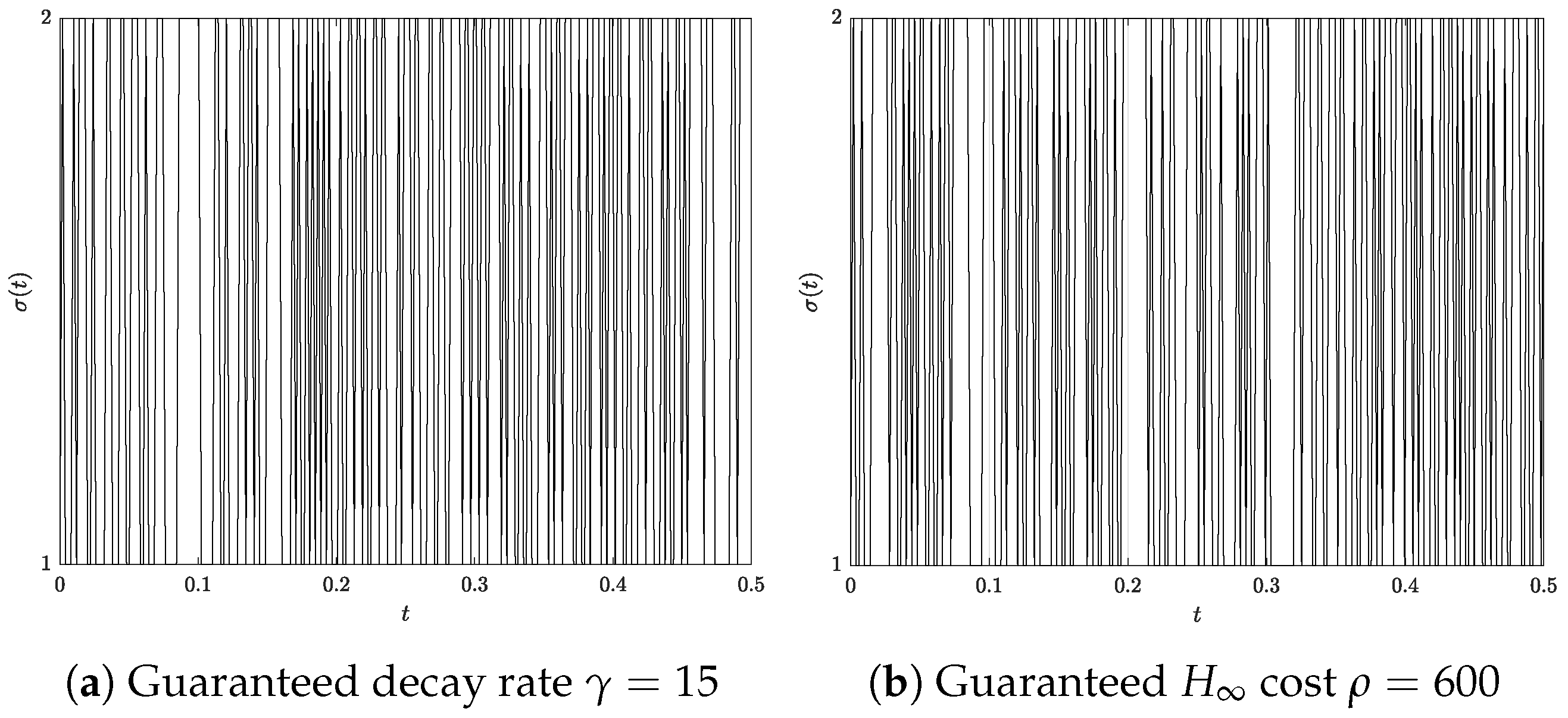
3.1. Guaranteed Decay Rate

The state estimation convergence is evaluated within a Lyapunov framework, considering a minimum-type piecewise quadratic Lyapunov function [29]. The analysis of the corresponding dissipation mechanism leads to a set of LMI conditions for the purpose of the switched observer design. To this end, let $V:{\mathbb{R}}^{n_x}\to {\mathbb{R}}^{+}$ be the (positive definite) weight functional candidate as defined below:

$$\begin{array}{cc}\hfill V\left(\tilde{x}\left(t\right)\right)& =\underset{i\in \{1,...,n_p\}}{\min }{\tilde{x}}^T\left(t\right)P_i\tilde{x}\left(t\right)\hfill \\ \hfill & =\underset{\lambda \in \Lambda }{\min }\left(\sum _{i=1}^{n_p}{\lambda }_i{\tilde{x}\left(t\right)}^T{P}_i\tilde{x}\left(t\right)\right)\hfill \end{array}$$

(20)

where $P_i>0\in {\mathbb{S}}^{n_x}$$\forall i\in \{1,...,n_p\}$. In order to ensure the convergence of the estimated states, consider the following dissipation inequality:

$$D^{+}V\left(t\right)+2\gamma V\left(t\right)\le 0,$$

(21)

where $\gamma$ is a positive scalar and $D^{+}V\left(t\right)$ denotes the Dini time derivative [34] of the piecewise Lyapunov function in (20). If (21) is satisfied along the trajectories of (10), the estimation error dynamics are exponentially stable with a guaranteed decay rate $\gamma$, since it can be readily shown that the following holds

$$\parallel \tilde{x}\left(t\right)\parallel \le M_x\parallel \tilde{x}\left(0\right)\parallel {\mathrm{e}}^{-\gamma t}$$

(22)

for every $\tilde{x}\left(0\right)\in \tilde{\mathcal{X}}\subset {\mathbb{R}}^{n_x}$.

Problem 1.

Determine a switching strategy $\sigma (·):{\mathbb{R}}^{n_y}\to \{1,...,n_s\}$ such that: $\sigma (·)=\varphi \left(y\right(t\left)\right)$, $\forall ,t\ge 0$, which makes the origin $\tilde{x}=0$ of the error system (10), supposing that $d\left(t\right)=0$ for $t\ge 0$, an exponentially stable equilibrium point.

A solution for Problem 1 is presented in the following theorem.

Theorem 1.

Consider the error dynamics defined in (10). Let μ and γ be given positive scalars, Suppose there exist $P_i\in {\mathbb{S}}^{n_x}$, $Q_i\in {\mathbb{S}}^{n_y}$, $M_i\in {\mathbb{R}}^{n_x\times n_y}$, $i=1,\dots ,n_p$, such that

$$\begin{array}{cc}\hfill & P_i>0,i=1,\dots ,n_p\hfill \end{array}$$

(23)

$$\begin{array}{cc}\hfill & {\mathrm{H}}_{\mathrm{e}}\{P_i{A}_j+M_{i}C\}+\mu C^T(Q_j-Q_i)C+2\gamma P_i<0,i,j=1,\dots ,n_p\hfill \end{array}$$

(24)

Then, the estimation error dynamics are locally exponentially stable with a guaranteed decay rate γ, with the switching strategy as defined in (13) and the following observer gains:

$$L_i=P_i^{-1}{M}_i,i=1,...,n_p.$$

(25)

Proof. 

Multiplying (23) by ${\alpha }_j$, summing up all terms for all $j\in \{1,...,n_p\}$, and considering (16), yields

$${(A\left(\alpha \right)+L_{i}C)}^T{P}_i+P_i(A\left(\alpha \right)+L_{i}C)+2\gamma P_i+C^T\left(\sum _{j=1}^{n_p}{\pi }_{ji}\left(\alpha \right)Q_j\right)C<0.$$

(26)

Pre- and post-multiplying (26) by the vector $x^T\left(t\right)$ and its transpose, respectively, yields

$${\tilde{x}}^T\left(t\right)〔{(A\left(\alpha \right)+L_{i}C)}^T{P}_i+P_i(A\left(\alpha \right)+L_{i}C)+2\gamma P_i〕\tilde{x}\left(t\right)<-{\tilde{y}}^T\left(t\right)\left(\sum _{j=1}^{n_p}{\pi }_{ji}\left(\alpha \right)Q_j\right)\tilde{y}\left(t\right)$$

(27)

Considering that $i\in \mathcal{I}\left(\tilde{y}\left(t\right)\right)$, we obtain  

$${\tilde{y}}^T\left(t\right)\left(\sum _{j=1}^{n_p}{\pi }_{ji}\left(\alpha \right)Q_j\right)\tilde{y}\left(t\right)>0$$

(28)

and then, from (27), the following sufficient conditions are true

$${\tilde{x}}^T\left(t\right)〔{(A\left(\alpha \right)+L_{i}C)}^T{P}_i+P_i(A\left(\alpha \right)+L_{i}C)+2\gamma P_i〕\tilde{x}\left(t\right)<0$$

(29)

On the other hand, for the quadratic Lyapunov candidate function defined in (20), the RHS of the dissipation inequality (21) satisfies

$$\begin{array}{c}{D}^{+}V\left(t\right)+2\gamma V\left(t\right)=\underset{l\in I\left(x\right(t\left)\right)}{\min }{\tilde{x}}^T\left(t\right)〔{(A\left(\alpha \right)+L_{i}C)}^T{P}_i+P_i(A\left(\alpha \right)+L_{i}C)+2\gamma P_i〕\tilde{x}\left(t\right)\hfill \\ \hfill \le {\tilde{x}}^T\left(t\right)〔{(A\left(\alpha \right)+L_{i}C)}^T{P}_i+P_i(A\left(\alpha \right)+L_{i}C)+2\gamma P_i〕\tilde{x}\left(t\right).\end{array}$$

(30)

It follows that (29) implies

$$D^{+}V\left(t\right)+2\gamma V\left(t\right)<0$$

(31)

and hence (22) is fulfilled and the proof is completed.    □

3.2. $H_{\infty }$ Guaranteed Cost

Next, we address the non-linear $H_{\infty }$ switched observer design problem when $d\left(t\right)\ne 0$ by defining an output performance vector $z\left(t\right)=E\tilde{x}\left(t\right)$, with $z\in {\mathbb{R}}^{n_z}$ and $E\in {\mathbb{R}}^{n_z\times n_x}$, which, along with the error dynamics, yields

$$\begin{array}{cc}\hfill \dot{\tilde{x}}\left(t\right)& =(A\left(\alpha \left(t\right)\right)+L_{\sigma \left(t\right)}C)\tilde{x}\left(t\right)+B_{d}d\left(t\right)\hfill \\ \hfill z\left(t\right)& =E\tilde{x}\left(t\right).\hfill \end{array}$$

(32)

Then, the ${\mathcal{L}}_2$-gain of the non-linear error dynamics (often referred as the $H_{\infty }$ cost) can be defined as follows:

$$J_{\infty }:=\underset{0\ne d\in {\mathcal{L}}_2}{sup}{\displaystyle \frac{{∥z∥}_2^2}{{∥d∥}_2^2}}.$$

(33)

which allows us to formulate the following problem.

Problem 2.

Determine a switching strategy $\sigma (·):{\mathbb{R}}^{n_y}\to \{1,...,n_p\}$, with $\sigma (·)=\varphi \left(y\right(t\left)\right)$, which guarantees that the origin of the unforced estimation error dynamics, i.e., the system defined in (10) with $d\left(t\right)=0$, is locally exponentially stable while ensuring that

$$\underset{d\in {\mathcal{L}}_2}{sup}{\displaystyle \frac{{∥z∥}_2^2}{{∥d∥}_2^2}}<\rho$$

(34)

for a given $\rho >0$.

A solution for Problem 2 is proposed in the following theorem

Theorem 2.

Consider the error dynamics in (32). Let μ and γ be given positive scalars. Suppose there exists $P_i\in {\mathbb{S}}^{n_x}$, $Q_i\in {\mathbb{S}}^{n_y}$, $M_i\in {\mathbb{R}}^{n_x\times n_x}$, $i=1,\dots ,n_p$, and $\rho \in \mathbb{R}$ such that the following is satisfied:

$$\begin{array}{cc}\hfill & P_i>0,i=1,\dots ,n_p\hfill \end{array}$$

(35)

$$\begin{array}{cc}\hfill & \left[\begin{array}{ccc}{\Pi }_{i,j}& P{B}_d& E^T\\ B_d^{T}P& -\rho I& 0\\ E& 0& -I\end{array}\right]<0,i,j=1,\dots ,n_p\hfill \end{array}$$

(36)

where

$${\Pi }_{i,j}={\mathrm{H}}_{\mathrm{e}}\{P_i{A}_j+M_{i}C\}+\mu C^T(Q_j-Q_i)C.$$

Then, the switching strategy defined in (13) with $L_i=P_i^{-1}{M}_i$, $i=1,\dots ,n_p$, guarantees that the origin of the estimation error dynamics defined in (8) with $d\left(t\right)=0$ is locally exponentially stable and $J_{\infty }\le \rho$.

Proof. 

Multiplying (35) by ${\alpha }_j$, summing up all terms for all $j\in \{1,...,n_p\}$, yields

$$\left[\begin{array}{ccc}\Pi {\left(\alpha \right)}_{i,j}& P{B}_d& E^T\\ B_d^{T}P& -\rho I& 0\\ E& 0& -I\end{array}\right]<0$$

(37)

with

$$\Pi {\left(\alpha \right)}_{i,j}={\mathrm{H}}_{\mathrm{e}}\{PA\left(\alpha \right)+M_{i}C\}+C^T\left(\sum _{j=1}^{n_p}{\pi }_{ji}\left(\alpha \right)Q_j\right)C.$$

Performing the Schur complement in (37) and rearranging the terms, we obtain

$$\left[\begin{array}{cc}\Pi {\left(\alpha \right)}_{i,j}& P{B}_d\\ B_d^{T}P& -\rho I\end{array}\right]+\left[\begin{array}{c}{E}^T\\ 0\end{array}\right]\left[\begin{array}{cc}E& 0\end{array}\right]<0.$$

(38)

Pre- and post-multiplying (38) by the vector $\left[x{\left(t\right)}^{T}d{\left(t\right)}^T\right]$ and its transpose, respectively, yields

$$\begin{array}{c}{\tilde{x}}^T\left(t\right)〔{(A\left(\alpha \right)+L_{i}C)}^T{P}_i+P_i(A\left(\alpha \right)+L_{i}C)+E^{T}E〕\tilde{x}\left(t\right)+{\tilde{x}}^T\left(t\right)P{B}_{d}d\left(t\right)\\ +d^T\left(t\right)B_{d}P\tilde{x}\left(t\right)-\rho d^T\left(t\right)d\left(t\right)<-{\tilde{y}}^T\left(t\right)\left(\sum _{j=1}^{n_p}{\pi }_{ji}\left(\alpha \right)Q_j\right)\tilde{y}\left(t\right).\end{array}$$

(39)

According to the definition in $i\in \mathcal{I}\left(\tilde{y}\left(t\right)\right)$, from (39), the following condition is true

$$D^{+}V\left(t\right)+z^T\left(t\right)z\left(t\right)-\rho d^T\left(t\right)d\left(t\right)<0.$$

(40)

Rearranging and integrating each element in the inequality above from $t=0$ to $t\to \infty$ yields

$${\parallel z\left(t\right)\parallel }^2-\rho {\parallel d\left(t\right)\parallel }^2<V\left(0\right)-V(\infty )$$

(41)

and under zero initial conditions $V\left(0\right)=0$, one has

$${\displaystyle \frac{{∥z\left(t\right)∥}_2^2}{{∥d\left(t\right)∥}_2^2}}<\rho .$$

(42)

Hence, the proof is concluded.    □

Remark 1.

Notice that the term $\mu C^T(Q_j-Q_i)C$ included in the conditions (23) and (35) of the previous theorems may be cast as BMIs since $Q_i$ and μ are decision variables. However, if the parameter $\mu >0$ is set to be known, those conditions become standard LMIs. Further, a proposed algorithm will exploit the optimisation of the parameters μ in order to achieve suboptimal values for the guaranteed $H_{\infty }$ cost.

3.3. Stability Regions

A practical way of determining regions of stability comes from Lyapunov Theory [35]. It is well known that if $V\left(\tilde{x}\left(t\right)\right)$ is a Lyapunov function, such that $\dot{V}\left(\tilde{x}\left(t\right)\right)<0$, $\forall \tilde{x}\in \tilde{X}\subset {\mathbb{R}}^{n_x}$ along the trajectories of the system, and $\tilde{X}$ is a set containing the origin in its interior. In addition, to derive computationally tractable solutions, the state error domain $\tilde{X}$ may be constrained to be a given polytopic set as defined below

$$\tilde{X}=\left\{\tilde{x}\in {\mathbb{R}}^{n_x}:c_k^T\tilde{x}\le 1,k=1,...,n_g\right\}$$

(43)

where $c_1,...,c_{n_g}\in {\mathbb{R}}^{n_x}$ define the $n_g$ faces of $\tilde{X}$.

To apply the result presented in [35], we have to determine the largest contour curve of the Lyapunov function

$$\begin{array}{c}\hfill V\left(x\left(t\right)\right)=\underset{i\in \{1,...,n_p\}}{\min }{\tilde{x}}^T\left(t\right)P_i\tilde{x}\left(t\right)\end{array}$$

(44)

Hence, the following developments are instrumental for the derivation of results to determine estimates of the basin of attraction, using ellipsoidal domains contained in the set $\tilde{X}$. With this aim, we can normalize the associated level sets [35]

$$\tilde{\mathcal{X}}=\left\{\tilde{x}\in {\mathbb{R}}^{n_x}:V\left(x\right)\le \eta \right\},\mathrm{with}\eta >0,$$

(45)

to be given by ellipsoidal domains ${\tilde{\mathcal{X}}}_i$ defined as follows:

$${\tilde{\mathcal{X}}}_i=\left\{\tilde{x}\in {\mathbb{R}}^{n_x}:{\tilde{x}}^T{P}_i\tilde{x}\le 1\right\}$$

(46)

and seek an LMI formulation for the inclusion problem ${\tilde{\mathcal{X}}}_i\subset \tilde{X}$. This inclusion relationship may be rewritten as

$$\begin{array}{cc}\hfill & 2-c_k^{T}x-x^T{c}_k\ge 0,k=1,...,n_g\hfill \\ \hfill & \forall \tilde{x}:{\tilde{x}}^T{P}_i\tilde{x}-1\le 0,i=1,...,n_p\hfill \end{array}$$

(47)

then, applying the S-procedure [36] to the last set of inequalities, we obtain

$$\begin{array}{cc}\hfill & {\left[\begin{array}{c}1\\ -x\end{array}\right]}^T\left[\begin{array}{cc}1& c_k^T\\ c_k& P_i\end{array}\right]\left[\begin{array}{c}1\\ -x\end{array}\right]\ge 0,\hfill \\ \hfill & i=1,...,n_p,k=1,...,n_g.\hfill \end{array}$$

(48)

The above condition is satisfied if there is a solution feasible for the following LMI:

$$\begin{array}{cc}\hfill 1-c_k^T{P}_i{c}_k& \ge 0,\hfill \\ \hfill i=1,...,n_p,& k=1,...,n_g.\hfill \end{array}$$

(49)

3.4. Limited Observer Gain Norm

In actual applications, it is frequently undesirable for the LMI-based observer design to yield high observer gains. Since $L_{\sigma }$ is not a decision variable, we are unable to directly restrict it; instead, we must limit its norm. Specifically, let $\chi$ be the highest permitted norm for the observer gain $L_{\sigma }$. Thus, the  following inequality holds

$$L_i^T{L}_i=M_i^T{P}_i^{-2}{M}_i\le \chi I$$

From the Schur complement, we obtain

$$\left[\begin{array}{cc}\chi I& M_i^T\\ M_i& P_i^2\end{array}\right]\ge 0.$$

(50)

As the matrix inequality in (50) quadratically depends on the decision variable P, we propose the following relaxation

$$P_i-ϵI\ge 0\left[\begin{array}{cc}\chi I& M_i^T\\ M_i& {ϵ}^{2}I\end{array}\right]\ge 0$$

(51)

that has to be jointly solved along with the above LMIs in order to confine the norm of $L_i$, with $ϵ>0$ denoting a given small positive scalar that the designer will assign.

On the other hand, an optimization problem may be used to find a solution to the stabilization problem that maximizes the estimation $\tilde{\mathcal{X}}$ of the stability region. Since $\widetilde{{\mathcal{X}}_i}$ is an ellipse, we can maximize the volume of $\tilde{\mathcal{X}}$ by formulating an convex optimization problem. An algorithm for the switched observer design with an estimate stability region is provided below, based on the preceding developments.

Remark 2.

Notice that Algorithm 1 sets noteworthy improved features on a flexible design framework in terms of LMIs by ensuring not only exponential stability and guaranteed $H_{\infty }$ cost for the estimation error dynamics, but also optimum guaranteed stability regions of convergence.

Algorithm 1: Switched Observer Design with Guaranteed Stability Region

Build vectors ${\tilde{c}}_1,...,{\tilde{c}}_{n_g}$ that characterize the polytopic set $\tilde{X}$ as given by (43). Build the matrices $A_1,...,A_{n_p}$, which define the polytopic matrix in (11). For the purpose of obtaining an optimized estimate of the stability region, we consider the following convex optimization problem $$\underset{i\in \{1,...,n_p\}}{\min }\underset{M_i,Q_i}{\max }log\det \left(P_i\right)$$ (52) subject to (a) (23), (48), about the setting in which Theorem 1 is applied, and (51) for the state estimation with prescribed decay rate $\gamma$ and an upper bound $\chi$ for the switched observer gain matrices norm. (b) (35), (48), about the setting in which Theorem 2 is applied, and (51) for the state estimation with upper bounds $\rho$ and $\chi$ for the $H_{\infty }$ cost and the switched observer gain matrices norm, respectively.

4. Simulation Results

In this section, we illustrate the proposed observer design procedure through a numerical example. Consider a one link manipulator with revolute joints actuated by a DC motor. The elasticity of the joint may be well-modeled by a linear tensional spring. The elastic coupling of the motor shaft to the link introduces an additional degree of freedom. The states of this system are motor position and velocity, and the link position and velocity. The corresponding state-space model is

$$\begin{array}{cc}\hfill {\dot{\theta }}_m& ={\omega }_m\hfill \\ \hfill {\dot{\omega }}_m& ={\displaystyle \frac{k}{J_m}}({\theta }_1-{\theta }_m)-{\displaystyle \frac{B}{J_m}}{\omega }_m+{\displaystyle \frac{K_{\tau }}{J_m}}\tau \hfill \\ \hfill {\dot{\theta }}_1& ={\omega }_1\hfill \\ \hfill {\dot{\omega }}_1& =-{\displaystyle \frac{k}{J_1}}({\theta }_1-{\theta }_m)-{\displaystyle \frac{mgh}{J_1}}sin\left({\theta }_1\right)\hfill \end{array}$$

(53)

where ${\theta }_m$, ${\omega }_m$, ${\theta }_l$ and ${\omega }_l$ are the motor and link position and velocities, respectively. $J_m$ and $J_l$ are the inertia of the motor and link, respectively, h, and M represent the length and mass of the link, b is the viscous friction, and $K_{\tau }$ is the amplifier gain. The torque due to the stiffening spring is $\tau$.

The system modeled by (53) takes the form of (3) by considering

$$\begin{array}{cc}\hfill & x\left(t\right)={\left[\begin{array}{cccc}{\theta }_m\left(t\right)& {\omega }_m\left(t\right)& {\theta }_l\left(t\right)& {\omega }_l\left(t\right)\end{array}\right]}^T\hfill \\ \hfill & A={\left[\begin{array}{cccc}0& 1& 0& 0\\ -{\displaystyle \frac{k}{J_m}}& -{\displaystyle \frac{B}{J_m}}& {\displaystyle \frac{k}{J_m}}& 0\\ 0& 0& 0& 1\\ -{\displaystyle \frac{k}{J_1}}& 0& {\displaystyle \frac{k}{J_1}}& 0\end{array}\right]}^T,\hfill \\ \hfill & B_f={\left[\begin{array}{cccc}0& 0& 0& -{\displaystyle \frac{mgh}{J_1}}\end{array}\right]}^T,B_u={\left[\begin{array}{cccc}0& {\displaystyle \frac{K_{\tau }}{J_m}}& 0& 0\end{array}\right]}^T\hfill \\ \hfill & f\left(x\left(t\right)\right)=sin\left(x_3\left(t\right)\right).\hfill \end{array}$$

(54)

The adopted numerical values for the process parameters are taken from

Table 1. Parameter values.

Parameters	Numerical Values
$J_m$	$3.7\times {10}^{-3}$ kg m2
$J_l$	$9.3\times {10}^{-3}$ kg m2
h	$1.5\times {10}^{-1}$ m
m	$0.21$ kg
B	$4.6\times {10}^{-2}$ m
$K_{\tau }$	$8\times {10}^{-2}$ Nm/V
k	1 Nm/rad
g	$9.8$ m/s2

.

Applying our approach, we obtain

$$\begin{array}{cc}\hfill h_{1,j}& =0,j=1,2,3\hfill \\ \hfill h_{1,3}& =-3.33cos\left({\breve{x}}_3\left(t\right)\right)\hfill \end{array}$$

(55)

then

$$\begin{array}{cc}\hfill {\overline{h}}_{1,3}& =-3.33\hfill \\ \hfill {\underline{h}}_{1,3}& =3.33\hfill \end{array}$$

which defines the set of matrix vertices of the uncertain polytopic matrix $A\left(\alpha \right)$ in (11) as follows

$$\begin{array}{cc}\hfill A_1& =\left(\begin{array}{cccc}0& 1.0& 0& 0\\ -270.3& -12.43& 270.3& 0\\ 0& 0& 0& 1.0\\ -107.5& 0& 218.1& 0\end{array}\right)\hfill \\ \hfill A_2& =\left(\begin{array}{cccc}0& 1.0& 0& 0\\ -270.3& -12.43& 270.3& 0\\ 0& 0& 0& 1.0\\ -107.5& 0& -3.008& 0\end{array}\right)\hfill \end{array}$$

On the other side, $\tilde{X}$ defined in (43) is normalized considering the following polytopic set

$$\tilde{X}=\left\{\tilde{x}\in {\mathbb{R}}^4:|{\tilde{x}}_1|\le 0.5,|{\tilde{x}}_2|\le 0.25,|{\tilde{x}}_3|\le 0.5,|{\tilde{x}}_4|\le 0.5\right\}.$$

The procedure defined in Algorithm 1 is used to determine the appropriate selection of the design parameters. Thus, Figure 2 shows the feasibility region of the optimization problem (52) subject to the LMI conditions in (23), (48), and (51) with respect to $\mu$ and the upper bound of the decay rate $\gamma$, considering the cases given by $\chi =1.0\times {10}^5$, $\chi =5.0\times {10}^5$, $\chi =1.0\times {10}^6$, and $ϵ=0.01$ as parameters of design which allow the numerical implementability of the state observer.

Similarly, Figure 3 shows the feasibility region of the optimization problem (52) subject to the LMI conditions in (35), (48), and (51) under the same selection of design parameters.

As expected, Figure 2 and Figure 3 show that whenever the upper bound of the prescribed decay rate $\gamma$ and the guaranteed $H_{\infty }$ cost are set to be higher, respectively, the feasibility region associated with the solution of the corresponding convex optimization problem decreases for required low upper bound of the observer gain norm $\chi$. Moreover, no feasible region is obtained for $\chi =1.0\times {10}^5$ when the equivalent procedure with identical values of design parameters is applied in a non-switched implementation scheme of the observer design.

4.1. Optimized Initial Conditions

It is clear from this that the observer designer has two independent means for enhancing the condition that $\parallel \tilde{x}\left(t\right)\parallel$ in (22) promptly converges. First, the set of gain matrices $L_{\sigma }$ can be designed to make $\gamma$ as large as possible. Secondly, the value of $\widehat{x}\left(0\right)$ can be designed to minimize the ‘start-up error norm’

$$\parallel \tilde{x}\left(0\right)\parallel = \parallel x\left(0\right)-\widehat{x}\left(0\right)\parallel .$$

(56)

In particular, given that $x\left(0\right)$ is often unknown and by the virtue of the triangular inequality $\parallel x\left(0\right)-\widehat{x}\left(0\right)\parallel \le \parallel x\left(0\right)\parallel +\parallel \widehat{x}\left(0\right)\parallel$, we have that our objective implies the minimization of $\parallel \widehat{x}\left(0\right)\parallel$. Then, the physically realizable design is related to meet the initial measurements $y\left(0\right)$, which are assumed to be known. Thus, the solution of the following semi-definite programming (SDP) problem

$$\begin{array}{cc}\hfill & \min \parallel \widehat{x}\left(0\right)\parallel \hfill \\ \hfill & \text{subject to}\hfill \\ \hfill & \left\{\begin{array}{c}C\widehat{x}\left(0\right)=y\left(0\right)\hfill \end{array}\right.\hfill \end{array}$$

(57)

Thus, the solution of (57) may be addressed by using conventional quadratic programming tools providing a local optimal selection for $\widehat{x}\left(0\right)$.

4.2. Observer Tests

The observer and system responses are generated via numerical simulation with initial profiles $x_0=\left[\begin{array}{cccc}1& 0& 1& 0\end{array}\right]$ and ${\widehat{x}}_0$ obtained from the optimization problem (57).

Figure 4 shows the evolution of the estimation error norm for both estimation schemes: guaranteed $H_{\infty }$ cost (with $d\left(t\right)$ selected as a unitary pulse in $t=0.05$), $\rho$, and upper bound decay rate $\gamma$ ($d\left(t\right)=0$) for the design parameters $\chi =5.0\times {10}^5$ and $ϵ=0.01$. Furthermore, plots that result from the implementation of observers with constant injection gains are shown for comparison purposes. We can observe that the error evolution is indeed bounded and exponentially convergent in both cases, but with an enhanced performance when switching gains are implemented. Since the initial estimation profiles are already a good approximation of the actual variable states, the estimation error norm converges quickly, and hence, provides very satisfactory estimates.

Furthermore, Figure 5 depicts the switching among the available output injection gains, which triggers an enhanced performance of the estimates.

5. Concluding Remarks

In this work, we have proposed an switched observer design for semi-linear systems. Specifically, an uncertain polytopic linear equivalent model for the semi-linear estimate error dynamics equations has been derived using the LPV formulation method. Then, an LMI-based condition was proposed for designing a non-linear Luenberger observer considering a switching rule that selects the adequate observer gain along the course of system operation. In addition, a stability region estimation algorithm (embedded into the observer design) was also proposed to properly select the initial condition of the estimation error. The proposed results were illustrated and numerically tested with a representative case example. It has been clearly noted that the proposed observer provides accurate estimation of the states via the computationally tractable state observer design based on convex optimization tools, such as LMIs. The switched observer design from the LPV formulation for the non-linear estimation error dynamics as presented in [11] allow us to increase the feasibility regions for the design parameters associated to the LMI conditions, which increases the flexibility of the design. These design features provide meaningful improvements when compared to similar approaches taken from specialized literature [37] in which the LPV formulations with constant observer gains are approached, yielding conservative designs in a smaller feasibility region of the design parameters.

References

1. Kang, W.; Krener, A.J.; Xiao, M.; Xu, L. A survey of observers for nonlinear dynamical systems. In Data Assimilation for Atmospheric, Oceanic and Hydrologic Applications (Vol. II); Springer: Berlin/Heidelberg, Germany, 2013; pp. 1–25. [Google Scholar]
2. Radke, A.; Gao, Z. A survey of state and disturbance observers for practitioners. In Proceedings of the 2006 American Control Conference, Minneapolis, MN, USA, 14–16 June 2006; pp. 6–11. [Google Scholar]
3. Bernard, P.; Andrieu, V.; Astolfi, D. Observer design for continuous-time dynamical systems. Annu. Rev. Control 2022, 53, 224–248. [Google Scholar] [CrossRef]
4. Zhang, X.M.; Han, Q.L. State estimation for static neural networks with time-varying delays based on an improved reciprocally convex inequality. IEEE Trans. Neural Netw. Learn. Syst. 2017, 29, 1376–1381. [Google Scholar] [CrossRef] [PubMed]
5. Zhang, X.M.; Han, Q.L.; Ge, X. Sufficient conditions for a class of matrix-valued polynomial inequalities on closed intervals and application to H filtering for linear systems with time-varying delays. Automatica 2021, 125, 109390. [Google Scholar] [CrossRef]
6. Zemouche, A.; Rajamani, R. Observer design for non-globally lipschitz nonlinear systems using hilbert projection theorem. IEEE Control Syst. Lett. 2022, 6, 2581–2586. [Google Scholar] [CrossRef]
7. Phanomchoeng, G.; Rajamani, R. Observer design for Lipschitz nonlinear systems using Riccati equations. In Proceedings of the 2010 American Control Conference, Baltimore, MD, USA, 30 June–2 July 2010; pp. 6060–6065. [Google Scholar]
8. Papageorgiou, P.C.; Alexandridis, A.T. A New Approach for Designing Stable Nonlinear bounded-Lipschitz Observers. In Proceedings of the 2020 28th Mediterranean Conference on Control and Automation (MED), Saint-Raphaël, France, 16–18 September 2020; pp. 150–155. [Google Scholar]
9. Zhang, W.; Su, H.; Zhu, F.; Azar, G.M. Unknown input observer design for one-sided Lipschitz nonlinear systems. Nonlinear Dyn. 2015, 79, 1469–1479. [Google Scholar] [CrossRef]
10. Arefanjazi, H.; Ataei, M.; Ekramian, M.; Montazeri, A. A robust distributed observer design for Lipschitz nonlinear systems with time-varying switching topology. J. Frankl. Inst. 2023, 360, 10728–10744. [Google Scholar] [CrossRef]
11. Zemouche, A.; Boutayeb, M. On LMI conditions to design observers for Lipschitz nonlinear systems. Automatica 2013, 49, 585–591. [Google Scholar] [CrossRef]
12. Phanomchoeng, G.; Rajamani, R.; Piyabongkarn, D. Nonlinear observer for bounded Jacobian systems, with applications to automotive slip angle estimation. IEEE Trans. Autom. Control 2011, 56, 1163–1170. [Google Scholar] [CrossRef]
13. Lam, H.; Leung, F.H.; Tam, P.K. A switching controller for uncertain nonlinear systems. IEEE Control Syst. Mag. 2002, 22, 7–14. [Google Scholar]
14. Li, S.; Ahn, C.K.; Xiang, Z. Command-filter-based adaptive fuzzy finite-time control for switched nonlinear systems using state-dependent switching method. IEEE Trans. Fuzzy Syst. 2020, 29, 833–845. [Google Scholar] [CrossRef]
15. Niu, B.; Zhao, P.; Liu, J.D.; Ma, H.J.; Liu, Y.J. Global adaptive control of switched uncertain nonlinear systems: An improved MDADT method. Automatica 2020, 115, 108872. [Google Scholar] [CrossRef]
16. Elias, L.J.; Faria, F.A.; Magossi, R.F.; Oliveira, V.A. Switched control design for nonlinear systems using state feedback. J. Control Autom. Electr. Syst. 2022, 33, 733–742. [Google Scholar] [CrossRef]
17. Liu, C.; Wen, G.; Zhao, Z.; Sedaghati, R. Neural-network-based sliding-mode control of an uncertain robot using dynamic model approximated switching gain. IEEE Trans. Cybern. 2020, 51, 2339–2346. [Google Scholar] [CrossRef] [PubMed]
18. Rajamani, R.; Jeon, W.; Movahedi, H.; Zemouche, A. On the need for switched-gain observers for non-monotonic nonlinear systems. Automatica 2020, 114, 108814. [Google Scholar] [CrossRef]
19. Rajamani, R.; Jeon, W.; Movahedi, H.; Zemouche, A. Vehicle motion estimation using a switched gain nonlinear observer. In Proceedings of the 2020 American Control Conference (ACC), Denver, CO, USA, 1–3 July 2020; pp. 3047–3052. [Google Scholar]
20. Nouriani, A.; McGovern, R.A.; Rajamani, R. Step length estimation with wearable sensors using a switched-gain nonlinear observer. Biomed. Signal Process. Control 2021, 69, 102822. [Google Scholar] [CrossRef]
21. Ba, M.; Pianosi, P.; Rajamani, R. A switched-gain nonlinear observer for estimation of thoracoabdominal displacements and detection of asynchrony. Biomed. Signal Process. Control 2024, 96, 106494. [Google Scholar] [CrossRef]
22. N’Doye, I.; Zhang, D.; Zemouche, A.; Rajamani, R.; Laleg-Kirati, T.M. A switched-gain nonlinear observer for LED optical communication. IFAC-PapersOnLine 2020, 53, 4941–4946. [Google Scholar] [CrossRef]
23. Mohite, S.; Zemouche, A.; Haddad, M.; Alma, M.; Delattre, C.; Singh, N. H Switched-Gain Based Observer vs Nonlinear Transformation Based Observer for a Vehicle Tracking Model. IFAC-PapersOnLine 2021, 54, 126–131. [Google Scholar] [CrossRef]
24. Taghieh, A.; Mohammadzadeh, A.; Tavoosi, J.; Mobayen, S.; Rojsiraphisal, T.; Asad, J.H.; Zhilenkov, A. Observer-based control for nonlinear time-delayed asynchronously switching systems: A new LMI approach. Mathematics 2021, 9, 2968. [Google Scholar] [CrossRef]
25. Garbouj, Y.; Dinh, T.N.; Raissi, T.; Zouari, T.; Ksouri, M. Optimal interval observer for switched Takagi–Sugeno systems: An application to interval fault estimation. IEEE Trans. Fuzzy Syst. 2020, 29, 2296–2309. [Google Scholar] [CrossRef]
26. Tabbi, I.; Jabri, D.; Chekakta, I.; Belkhiat, D.E. Robust state and sensor fault estimation for switched nonlinear systems based on asynchronous switched fuzzy observers. Int. J. Adapt. Control Signal Process. 2024, 38, 90–120. [Google Scholar] [CrossRef]
27. Han, J.; Liu, X.; Wei, X.; Zhang, H. Adjustable dimension descriptor observer based fault estimation for switched nonlinear systems with partially unknown nonlinear dynamics. Nonlinear Anal. Hybrid Syst. 2021, 42, 101083. [Google Scholar] [CrossRef]
28. Zemouche, A.; Boutayeb, M.; Bara, G.I. Observer Design for Nonlinear Systems: An Approach Based on the Differential Mean Value Theorem. In Proceedings of the 44th IEEE Conference on Decision and Control, Seville, Spain, 12–15 December 2005; pp. 6353–6358. [Google Scholar]
29. Geromel, J.C.; Colaneri, P. Stability and stabilization of continuous-time switched linear systems. SIAM J. Control Optim. 2006, 45, 1915–1930. [Google Scholar] [CrossRef]
30. Lasdon, L.S. Optimization Theory for Large Systems; Dover Publications Inc.: Mineola, NY, USA, 2002. [Google Scholar]
31. Mohammadpour, J.; Scherer, C.W. Control of Linear Parameter Varying Systems with Applications; Springer Science & Business Media: Berlin/Heidelberg, Germany, 2012. [Google Scholar]
32. He, T.; Al-Jiboory, A.K.; Swei, S.S.M.; Zhu, G.G. Switching state-feedback LPV control with uncertain scheduling parameters. In Proceedings of the 2017 American Control Conference (ACC), Seattle, WA, USA, 24–26 May 2017; pp. 2381–2386. [Google Scholar]
33. Deaecto, G.S.; Geromel, J.C. Switched state feedback control for continuous-time polytopic systems and its relationship with LPV control. In Proceedings of the 2009 European Control Conference (ECC), Budapest, Hungary, 23–26 August 2009; pp. 2073–2078. [Google Scholar] [CrossRef]
34. Garg, K.M. Theory of Differentiation: A Unified Theory of Differentiation via New Derivate Theorems and New Derivatives; John Wiley & Sons: Hoboken, NJ, USA, 1998; Volume 28. [Google Scholar]
35. Khalil, H.K. Nonlinear Systems, 3rd ed.; Prentice Hall: Hoboken, NJ, USA, 2002. [Google Scholar]
36. Boyd, S.; El Ghaoui, L.; Feron, E.; Balakrishnan, V. Linear Matrix Inequalities in System and Control Theory; SIAM: Philadelphia, PA, USA, 1994. [Google Scholar]
37. Alaridh, I.; Aitouche, A.; Zemouche, A. Fault sensor detection and estimation based on LPV observer for vehicle lateral dynamics. In Proceedings of the 2018 7th International Conference on Systems and Control (ICSC), Valencia, Spain, 24–26 October 2018; pp. 71–77. [Google Scholar]
Figure 1. Switched observer implementation scheme.
Asi 07 00071 g001
Figure 2. Feasibility region for guaranteed decay rate γ with ϵ = 0.01 .
Asi 07 00071 g002
Figure 3. Feasibility region for guaranteed H cost ρ with ϵ = 0.01 .
Asi 07 00071 g003
Figure 4. Time evolution of the estimation error norm.
Asi 07 00071 g004
Figure 5. Time evolution of the swiching rule σ ( t ) .
Asi 07 00071 g005