Abstract
In a labor-intensive cell production system, it is important to train operators effectively because their skills are essential for productivity. Our previous study proposed a method to classify these skills according to a “skill index” based on the time required for each task and the allocated operators based on this method. However, in actual workplaces, it is assumed that operators accumulate fatigue due to the repetition of work, which affects the assembly time. In this study, we propose an operator allocation method that considers the effect of fatigue and verify its effectiveness compared with the results of the previous study by computer experiments. In addition, an assembly experiment with a toy is conducted based on the operator allocation method derived from the computer experiments. The experimental results show that the proposed method is effective and indicate that appropriate parameter setting is crucial when applying it in real-world scenarios.
1. Introduction
The manufacturing industry is transitioning from high-volume, low-volume production to high-mix, low-volume production (HMLV) [,,,] as consumer needs diversify. This transition requires more flexibility in the manufacturing process. Manual assembly operators remain essential in many manufacturing industries [] and they provide flexibility to the assembly line that is not possible with automated systems []. Manual handling is essential, especially in situations where flexibility is important.
Cell production systems are attracting attention as a form of production suitable for high-mix, low-volume production. In this system, operators are responsible for a wide range of tasks, and their skills have a significant impact on quality and productivity. Therefore, in cell production systems, it is important to accurately identify the skills of operators and effectively train them accordingly.
In recent years, the use of virtual reality (VR) and augmented virtual reality (AVR) technology has been reported as a training method to improve operators’ skills []. Qian-Wen Fu et al. (2024) [] study how to design VR systems to reduce cognitive load. Immersion in a virtual environment (VE) allows operators to experience the same emotions and sensations during training as they experience, such as the same anxiety, fear, and concern []. This is especially important in operations where a minor mistake can result in a serious accident []. Since this study targets simple assembly tasks, VR technology is not considered.
In the manufacturing industry, a skill management chart called a “skill map” is generally used to clarify the skills required for a task and to confirm and visualize the current skills of the operators. We proposed the “skill index”, which classifies operators’ skills based on the time required for a task, as a notation method for skill maps []. Operators become more proficient by repeating the same task, and the time required decreases. The skill index updates the skill level by estimating the time required to complete a task by simulating proficiency. However, in actual workplaces, it has been found that factors affecting assembly time are related to proficiency and other factors related to operator ability and the work environment [,]. These factors include age and experience, work design, and the effects of forgetting due to differences in the length of breaks separating work cycles [,,]. Furthermore, human factors, such as fatigue, affect the change in proficiency rate []. There are several learning models that incorporate fatigue parameters, which have been proposed by Asadayoobi et al. (2021) [], Mályusz et al. (2014) [], Digiesi et al. (2009) [], Knecht (1974) [], and Boone (2018) [], among others. In previous studies, these models were applied to datasets, and it was reported that the model by Asadayoobi et al. (2021) was the most effective [].
In this study, we focus on the effect of fatigue among various human factors to simulate more realistically a task-division-type multi-person cell production system. Haraguchi et al.’s method [] is used as the conventional method, and the method of Asadayoobi et al. [] is incorporated into the conventional method to propose an operator allocation method that considers the effects of fatigue. Therefore, the structure of this thesis is as follows: Section 2 describes the methodology used in the paper. Next, in Section 3, we design a specific mathematical model for the subject. In Section 4, we conduct computer experiments to verify the mathematical model’s properties; in Section 5, we conduct assembly experiments, which are important, to validate the model with the mathematical model. To ensure the fairness of the comparison of the two experiments, the computer experiments are conducted again in Section 5 under the same conditions as the assembly experiments. The final chapter, Section 6, summarizes this study.
2. Methods
2.1. Skill Index
In this study, the “skill index” proposed by Haraguchi et al. [] is used to represent the skills of operators. If the standard assembly time for each task of product is and the actual assembly time for each operator is , the skill index value is obtained by Equation (1).
For example, if the standard assembly time for Task 3 of Product 1 is 90 and the actual assembly time for Operator 2 is 100, the value of the skill index is 0.9. A smaller value for the skill index indicates that the operator is not good at the task, while a larger value indicates that the operator is good at the task. The skill index is used to classify operators’ skills into three levels: Newcomer, Standard, and Expert. Newcomers have , Standard operators have , and Experts have . This classification is based on the study of Haraguchi et al. []. The reduction in assembly time through learning can be significantly increased through repetition, but actual human skills are limited. Therefore, in this study, the upper limit of the skill index is set at 1.5 and the lower limit at 0.6.
In this study, the values of the skill index are used and assigned to tasks that require training. The skill index values of the assigned tasks are summed, and the smaller the value, the more difficult the task is assigned. This way, the training can be efficient. Ultimately, by aiming to build a highly robust group of operators, the project is expected to prevent productivity loss due to operator vacancies and reduce costs over the medium to long term.
2.2. Proficiency
Generally, as operators repeat the same task, the time required decreases. This phenomenon is called proficiency []. The learning curve represents an individual’s performance (time or cost) per repetitive task. Learning curves can predict the time required for an operator’s task and are typically used to optimize production planning and operator allocation. The learning curve has been studied quite a lot since it was first proposed by Wright []. The model proposed by Wright [] represents a constant percentage decrease in task time required for each doubling of cumulative output. Wright’s model is shown in Equation (2).
where is the assembly time of the unit, is the assembly time of the first unit, is the learning exponent, and is the learning rate. Wright’s learning curve has become a prominent model because of its simplicity and ability to fit a wide range of training data well [,,]. The learning curves at learning rates of 70%, 80%, and 90% are shown in Figure 1. Haraguchi et al. estimated skill index values by using Wright’s learning curve. Since the studies of Wright [], various learning curves have been developed, including exponential, hyperbolic, and S-shaped curves [,]. Several two- and three-parameter exponential function models have been developed [,,,]. The exponential model provides a more accurate production rate estimate than the log-linear model [,]. Anzanello and Fogliatto [] also showed that hyperbolic models are more robust than three-parameter exponential and time constant models []. The S-curve reflects three behaviors of performance. The learning curve is slow initially, steadily improves in the middle, and slows again when proficiency is reached []. A review of learning curves can be found in Yelle [], Dutton et al. [] and Dar-El [].
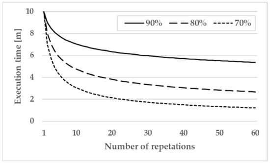
Figure 1.
Learning curve (learning rates of 70%, 80%, and 90%).
2.3. Learning Rate with Fatigue
The decrease in physical and cognitive resources that accompanies an increase in the number of tasks results in fatigue, which has been shown to negatively affect the progress of learning []. Accumulated fatigue can lead to a decline in operators’ judgment, decision making, and reaction time [,]. Furthermore, it has been shown that low levels of fatigue improve operator performance, while high levels of fatigue negatively affect operator performance [,]. Examples of tasks with high levels of fatigue include heavy-load tasks and tasks with long cycles [].
Asadayoobi et al. [] proposed Equation (4), which indicates a learning index that takes fatigue into account. This equation incorporates the effect of fatigue accumulation in the learning index by setting a fatigue index for each task. This is a crucial consideration, as fatigue accumulated through the repetition of tasks can deteriorate operator performance. Understanding and accounting for this factor is essential in our efforts to optimize operator performance.
where is learning index that varies with the number of iterations . is shown in Equation (3). Also, is the fatigue index, with . A small value of the fatigue index indicates a slow rate of fatigue accumulation, while a large value of the fatigue index indicates a fast rate of fatigue accumulation. The fatigue index is a task-specific value. By incorporating from Equation (4) into Equation (2), the assembly time of the th unit can be estimated, taking fatigue into account. Figure 2 shows the learning–fatigue curves when the learning rate is 80% and the fatigue index is 0.15, 0.20, and 0.25.
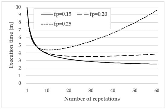
Figure 2.
Learning–fatigue curve (learning rate of 80%, fatigue index of 0.15, 0.20, 0.25).
From Figure 2, the accumulation of fatigue at the end of the workday results in a U-shaped curve. This is consistent with the study of Winkelhaus et al. [], who found that the performance of most operators subjected to learning and fatigue effects improved to a certain threshold and worsened beyond it.
3. The Target Model
3.1. Ditails
The target model is a labor-intensive cellular production system in which an operator’s skills play a major role in productivity. The features are as follows:
- The same order consisting of multiple products is received repeatedly.
- Each product is completely assembled in a single cell.
- More than one operator can be placed in a single cell, and operators must always be assigned to one of the cells.
- The operator is placed in only one cell.
- In the case of a multi-person cell, the cell shall be configured as a task-divided cell.
- Within the same cell, there is a task-dedicated assembly where only one person is assigned to a single task.
- If an operator is responsible for multiple tasks, the tasks should be performed consecutively.
- This is a job shop-type cell where the processing order of tasks varies for each product.
3.2. Symbols
Table 1 shows the symbols used to formulate the features in Section 3.1.

Table 1.
Symbols.
3.3. Formulation
In this study, we incorporate a learning index that accounts for fatigue when updating the skill index at the end of each order. In the study of Haraguchi et al. [], proficiency progressed as tasks were assigned, but in this study, skill improvement was hampered by fatigue depending on the number of tasks assigned. Therefore, tasks that each operator struggles with are assigned preferentially to facilitate skill proficiency. Consequently, the objective function is set to minimize the sum of the skill index for each task allocated to operators, as defined in Equation (5), where is the skill index values for each operator’s task, the decision variable represents who is assigned to which cell, and represents who is assigned to which task.
The constraints are defined by Equations (6)–(9). Equation (6) is the constraint that operators are always placed in one cell, and Equation (7) is the constraint that the maximum number of people in one cell must not exceed .
Equation (8) is a constraint that ensures that operators are assigned to adjacent tasks when they are responsible for multiple tasks.
In Equation (9), the number of operators who can be assigned to the same task within a cell is set to be one, achieving a task-dedicated system.
The tact time for each cell is calculated by Equation (10). Based on the tact time, the number of products to be assigned to each cell is determined by Equation (11).
The assembly time after the order completion is calculated based on the tasks assigned to the operators and the number of products. The conventional method [] is obtained by Equation (12) and the proposed method by Equation (13).
where in Equation (12) is calculated using Equation (3) and in Equation (13) is calculated using Equation (4).
4. Computational Experiments
In this section, we conduct computational experiments on the operator allocation method formulated in the previous chapter and compare it with conventional methods.
4.1. Solution Procedure
For each order, we determine the operator allocation, and the number of products allocated to each cell. Then, we update the skill index values based on the allocated tasks and number of products and determine the operator allocation and quantity of products for the following order. This is repeated until the order is completed. We use the Simulated Annealing (SA) algorithm to find a solution for each order. The Simulated Annealing (SA) algorithm is one of the effective probabilistic approximation methods for NP-hard problems, such as combinatorial optimization problems. As a feature, the variable called temperature is used. The higher the temperature, the greater the probability of accepting a worse solution, which helps prevent the algorithm from becoming stuck in a local optimum. As the temperature gradually decreases, the algorithm increasingly favors selecting better solutions. Figure 3 illustrates the solution procedure.
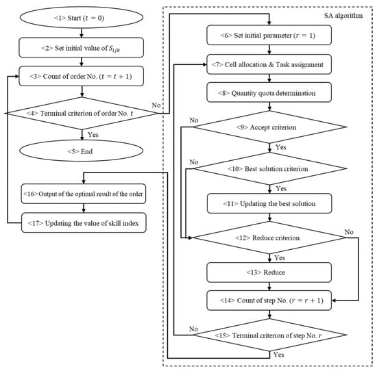
Figure 3.
Solution procedure.
First, we set the skill index values in <2>, and in <4>, we judge the terminal criterion for the number of orders t. After that, we enter the SA algorithm. After initializing the temperature and the number of steps in <6> (), the operators are allocated to each cell and task in <7>. After the number of products in each cell is determined in <8>, the solution acceptance judgment is performed in <9>. The acceptance judgment is determined by Equation (14), where is the current solution, is the following solution, and is the value of .
If , we update the best solution in <11>. If and is accepted, we do not update the best solution, and we proceed to the cooling judgment in <12>. represents the temperature at step . In <13>, the next temperature is set using Equation (15) with cooling rate .
The terminal criterion of the SA algorithm is determined by the number of steps . We return to <7> operator allocation and task assignment if the terminal criterion is not reached. After completing the step and terminating the SA algorithm, the best solution is output as the order t solution in <16>. Then, in <17>, based on the task assigned and the number of products assigned to each cell , the execution time is determined, and the skill index values are updated using Equations (12) and (13). This is repeated until the value of the order count t satisfies the termination criterion in <4>.
4.2. Conditions
Table 2 shows the configuration of the cells used in the experiment. The three cells (C1 to C3) are all equipped similarly and can accommodate either single or multiple cells. The total number of operators is eight (O1 to O8), and each cell can be staffed with one to four operators. The order details are as follows: there are three types of products (G1 to G3), four tasks for each type of product (K1 to K4), a quantity of 50 for each product, and five orders in total (T1 to T5).
Table 2.
Experimental conditions.
For the skill index, we use Table 3, which was used in the conventional method []. The eight operators consisted of two Expert operators, four Standard operators, and two Newcomer operators.
Table 3.
Operator’s skill index.
The learning rate was randomly set for each task in the range of 90% to 95%, as shown in Table 4.
Table 4.
Operator’s learning rate.
The fatigue index for all tasks is standardized using Patterns I to V, with values of 0.15, 0.20, 0.25, 0.30, and 0.35, respectively (Table 5).
Table 5.
Operator’s fatigue index.
The conditions for the Simulated Annealing (SA) used in the solution are as follows: The initial value is determined randomly, and the search progresses using the exchange neighborhood. The cooling rate is set at 0.95, with cooling performed every 100 steps. The termination criterion for each order is when the number of steps reaches 10,000. At the end of each order, the number of steps and the temperature are reset. One experiment consists of orders 1 through 5 (T1 to T5), and the experiments are conducted 20 times for each of the five fatigue index patterns of the proposed method and the conventional method for comparison.
4.3. Results
Figure 4 shows the progression of the best values in T1 of the first experiment for Patterns I to V of the proposed and conventional methods. In the initial phase of the number of steps, the proposed method has a smaller best value than the conventional method. However, after 1000 steps, the conventional method has a lower best value than the proposed method. The fastest to obtain the best solution was in Pattern III, with no variation from the 124th step onward. Subsequently, the best solutions were obtained in the order of the conventional method: Pattern II, Pattern I, Pattern V, and Pattern IV.
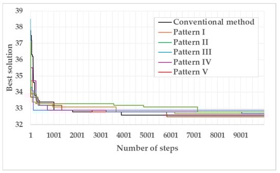
Figure 4.
Best values at order 1 of the first experiment for each pattern.
Table 6 shows the basic statistics of the minimum value of the sum of the skill index for each order for 20 trials for both the conventional method and Patterns I to V of the proposed method. In Table 6, the maximum average value for each order is indicated in red, and the minimum average is in blue. For the average values, Pattern III has the minimum value, and Pattern V has the maximum value for T1. For T2 to T5, Pattern V has the minimum value, and Pattern I has the maximum value. However, for T1, the average values are almost the same for both the proposed and conventional methods. The average value of T5 for Pattern I (=52.483) is closest to the maximum value of the sum of the skill index (=54), indicating that the operators have almost reached the Expert level. The average values of Patterns I and II of the proposed method exceeded those of the conventional method, and the gap widened as the orders progressed. For Patterns III to V of the proposed method, the average values were smaller than those of the conventional method from T2 onwards. For the conventional method and Patterns, I to III of the proposed methods, the value of the best solution increased as the order progressed, while for Patterns IV and V of the proposed method, the value of the best solution decreased as the order progressed.
Table 6.
Basic statistics of results.
4.4. Discussion of Computer Experiment
Table 6 shows that the average value of the best solution of the proposed method is smaller than that of the conventional method for Patterns III-V. Due to the influence of the fatigue index, the increase in actual assembly time after the completion of each order was reduced. Additionally, in Pattern IV and Pattern V of the proposed method, the value of the best solution decreased as the orders progressed. This is because the effect of the fatigue index exceeded that of proficiency. Therefore, by incorporating the fatigue index into Equation (13), it is possible to reflect not only the reduction in assembly time due to proficiency but also the negative impact of fatigue on assembly time.
On the other hand, Pattern I and Pattern II of the proposed method exceeded the average value of the conventional method as the orders progressed. A comparison of the learning rate values showed that the values of Pattern I and Pattern II of the proposed method were smaller than the values of the learning rate of the conventional method. Therefore, the progress of proficiency was faster in Pattern I and Pattern II of the proposed method than in the conventional method. This indicates that fatigue cannot be considered in some cases, depending on the combination of learning rate and fatigue index.
5. Assembly Experiment
To verify the effectiveness of the proposed method, this chapter compares the assembly time estimated by the proposed method with the assembly time obtained from an actual LEGO block robot assembly experiment. First, we conduct a computer simulation using the proposed method and then perform an actual assembly experiment according to the operator allocation that yielded the best value.
5.1. Experimental Subject
The subject work used in these experiments is shown in Figure 5. This robot is made of LEGO bricks, with 86 work elements and 163 parts. The entire process of the subject work was divided into four tasks (K1~K4). Figure 6 shows the subject’s work at the end of each task. The assembly time of the Standard operator was set as the standard assembly time. Table 7 shows the number of processes, parts, and standard assembly time for each task.
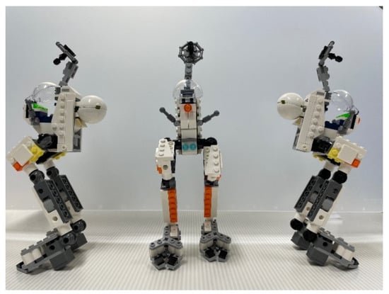
Figure 5.
A LEGO block robot used in the assembly experiment.
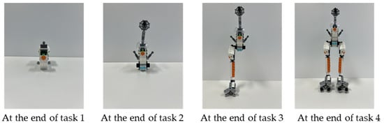
Figure 6.
A LEGO block robot after completion of each task in the assembly process.
Table 7.
The number of processes, parts and standard assembly time for each task.
5.2. Setting
Table 8 shows the composition of the cells subjected to the experiment. All three cells (C1 to C3) have equivalent facilities and can accommodate single and multiple cells. The number of operators is eight (O1 to O8), and the number of operators that can be placed in one cell is one to four. The order content is 1 (G1) for the product type, 4 (K1 to K4) for the number of tasks, and 30 for the order quantity. The operators consisted of two Experts, three Standards, and three Newcomers. Two subjects with the same operator composition (Group A and Group B) are tested. Since each operator’s exact skill index values are unknown, the midpoint value for each skill level is used. Additionally, since the exact values for the learning rate and fatigue index are unknown, they are all assumed to be constant. The learning rate was standardized to 93% for all operators and tasks, and the fatigue index was standardized to 0.20 for all tasks.
Table 8.
The composition of the cells.
5.3. Computational Experiment
The conditions of the Simulated Annealing (SA) used for the solution are the same as those described in Section 4.2. At the end of Order 1 (T1), the actual assembly time of the operator was updated, and the skill index was calculated. As a result of the experiment, the sum of the skill index for both Group A and Group B was 10.7. Table 9 shows the operator allocation and the number of products allocated to each cell for the best solutions in both Group A and Group B.
Table 9.
The operator allocation and the number of products allocated to each cell.
5.4. The Assembly Experiment
We set up an experimental cell production assembly station. Then, we assigned tasks according to the operator allocation obtained in the previous section and assembled a LEGO block. When an operator completes an assigned task, the work is handed over to the next operator for the subsequent task. After the previous task is completed, the operator of the next task starts assembling. The operator has a manual and a parts box for each task. The manual illustrates the parts and tasks for each assembly unit and is compiled into a booklet. The inside of the parts box is divided into partitions, and each section contains parts for 2–3 steps (Figure 7). The operators assemble the parts by referring to the manual and taking the parts from the parts box. Before the assembly experiment, Expert operators practiced assembly five times and Standard operators twice. The operators responsible for the Newcomers should have practiced in advance and participated in the experiment after receiving only brief guidance just before the experiment. During the experiment, a smartphone is placed on the workbench to record a video of the work conducted using an online meeting system. The assembly time was measured by watching the video after the experiment, and the assembly time per task was recorded for each operator.
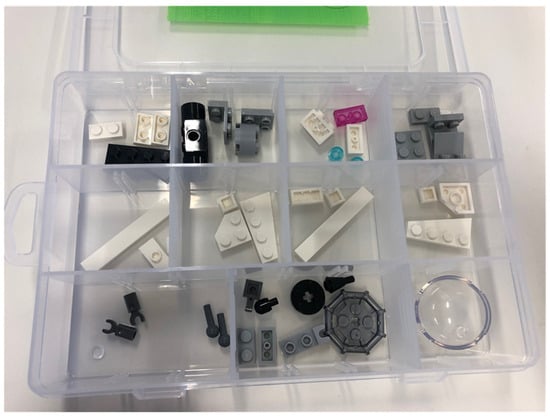
Figure 7.
Example of a parts box.
5.5. Comparison of Experimental Results
Table 10 shows the values of the skill index after the end of one order. The shaded cells represent the assigned tasks, and the skill index values have been updated. The values after the computational experiment were calculated from the post-training assembly times obtained using Equation (13) after the completion of the assigned tasks, and the values after the assembly experiment were calculated from the final assembly time. The skill index values after the computational experiment were higher than before. Expert operators reached the maximum value of the skill index (=1.50), Standard operators’ values were like the Experts’ and Newcomer operators’ values were like the Standard operators’.
Table 10.
Changes in the skill index.
On the other hand, after the assembly experiment, the values of the skill index were higher for the Standard and Newcomer operators than before the start of the work. The values were lower for all but one of the Expert operators. Looking at the differences in the skill index, the largest difference was 0.50 for the expert O1 in Group B, and the smallest difference was 0.00 for the skilled O2 in Group B. Additionally, it was found that the differences varied depending on the task, even for the same operator, indicating that the learning rate changes based on the type of work. The overall average of the difference was 0.037 and 0.039, and the standard deviation was 0.128 and 0.113, showing no significant differences between the groups.
Figure 8 provides a visual comparison of the assembly time for the computational and assembly experiments for each group. The final assembly time of the assembly experiment was generally shorter than that of the computational experiment, particularly for Group A in K3 and K4 of C1, K4 of C2, and K3 and K4 of C3, and for Group B, in K2 to K4 of C1, K2 and K4 of C2, and K4 of C3. However, in more than half of the tasks, the final assembly time of the assembly experiment exceeded that of the computational experiment. The degree of agreement between the assembly times of the two experiments varied depending on the task. For instance, for K3 of C1 in Group A and K2 and K3 of C2 in Group B, the data curves of the computational and assembly experiments were roughly consistent. In contrast, for K1 of C3 in Group A and K1 of C2 in Group B, there was a significant difference between the two data curves. In C2 of Group A and C3 of Group B, which had a larger number of work units, the data curves of the assembly experiment showed greater fluctuations.
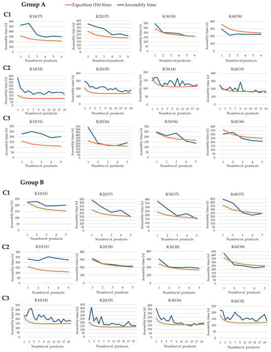
Figure 8.
The assembly time for the computational and assembly experiments for each group.
5.6. Discussion of Assembly Experiment
A comparison of the skill index of operators after the computer experiment and the assembly experiment shows differences. However, no significant difference was observed in the t-test, suggesting that the observed difference was not substantial. Examining the assembly time for each unit revealed that as the number of units increased, the variability in the assembly time of the assembly experiment also increased. The results show that there are other influences on the change in working time than proficiency and that the greater the number of repetitions of a task, the greater the effect. The skill index and proficiency rate values were estimated using the working time measured in the assembly experiment. The results differed from the values set before the experiment. Due to this, it is considered that there was a difference between the predicted assembly time and the actual assembly time. Therefore, when applying the proposed method to actual workplaces, it is essential to set appropriate parameters.
6. Conclusions
In this study, we proposed an operator allocation model that considers the decrease in proficiency due to fatigue. First, a comparison between the conventional method and the proposed method was conducted through computer simulations. The results show that the proposed method can consider the negative effects of working time due to fatigue and reduced working time due to proficiency. On the other hand, it was found that fatigue cannot be considered in some cases, depending on the combination of the fatigue index and the learning rate. More accurate simulation results can be expected by investigating the differences in results based on the combination of the learning rate and fatigue index.
Next, to verify the effectiveness of the proposed method, an actual assembly experiment was conducted based on the operator allocation obtained from the computer simulations, and the process of proficiency development was compared. As a result, although there was a difference between the calculated and measured assembly times, no significant difference was observed.
On the other hand, significant differences between operators were noted. This is considered to be due to the fact that, in this experiment, the operators’ skills and learning were treated uniformly. If the differences in the operators’ skills, learning rates, and fatigue indices can be considered, it is expected that the gap between the calculated values and the measured values will be reduced.
However, due to time constraints, this experiment was unable to individually consider each operator’s skill index, learning rate, and fatigue index. If these factors were to be considered, it would be possible to individually evaluate these parameters through preliminary experiments and incorporate them into the model. When applying this approach to a real-world setting, it is possible to calculate individual parameters by analyzing performance over several cycles of tasks; however, this may involve certain costs. Therefore, estimating general parameters based on specific workplace and task conditions and applying them to the model is considered a practical and cost-effective approach.
Future works will include creating a model that reflects differences in operators’ skill and proficiency, as well as developing a model that considers other human factors.
Author Contributions
Conceptualization, M.E. and H.H.; methodology, M.E.; software, M.E.; validation, M.E. and H.H.; data curation, M.E. and H.H.; writing—original draft preparation, M.E.; writing—review and editing, H.H. All authors have read and agreed to the published version of the manuscript.
Funding
The authors did not receive support from any organization for the submitted work.
Data Availability Statement
Raw data were generated at Author. Derived data supporting the findings of this study are available from the corresponding author H.H. on request.
Conflicts of Interest
The authors declare no conflict of interest.
References
- Katsuhisa, H.; Yasuaki, F.; Shin, S. A Study on the Workload in Cell Production. Jpn. J. Ergon. 2009, 45, 219–225. [Google Scholar]
- Gan, Z.L.; Musa, S.N.; Yap, H.J. A Review of the High-Mix, Low-Volume Manufacturing Industry. Appl. Sci. 2023, 13, 1687. [Google Scholar] [CrossRef]
- Abu-Samah, A.; Shahzad, M.K.; Zamai, E. Bayesian based methodology for the extraction and validation of time bound failure signatures for online failure prediction. Reliab. Eng. Syst. Saf. 2017, 167, 616–628. [Google Scholar] [CrossRef]
- Alduaij, A.; Hassan, N.M. Adopting a circular open-field layout in designing flexible manufacturing systems. Int. J. Comput. Integr. Manuf. 2020, 33, 572–589. [Google Scholar] [CrossRef]
- Fantini, P.; Tavola, G.; Taisch, M.; Barbosa, J.; Leitao, P.; Liu, Y.; Sayed, M.S.; Lohse, N. Exploring the integration of the human as a flexibility factor in CPS enabled manufacturing environments: Methodology and results. In Proceedings of the IECON 2016—42nd Annual Conference of the IEEE Industrial Electronics Society, Florence, Italy, 24–27 October 2016; pp. 5711–5716. [Google Scholar]
- Hoedt, S.; Claeys, A.; Aghezzaf, E.H.; Cottyn, J. Real Time Implementation of Learning-Forgetting Models for Cycle Time Predictions of Manual Assembly Tasks after a Break. Sustainability 2020, 12, 5543. [Google Scholar] [CrossRef]
- Nazir, S.; Totaro, R.; Brambilla, S.; Colombo, S.; Manca, D. Virtual Reality and Augmented-Virtual Reality as Tools to Train Industrial Operators. Comput. Aided Chem. Eng. 2012, 30, 1397–1401. [Google Scholar]
- Fu, Q.W.; Liu, Q.H.; Hu, T. Multi-objective optimization research on VR task scenario design based on cognitive load. Facta Univ. Ser. Mech. Eng. 2024, 22, 293–313. [Google Scholar] [CrossRef]
- Nazir, S.; Kluge, A.; Manca, D. Can Immersive Virtual Environments make the difference in training industrial operators? In Proceedings of the Human Factors and Ergonomics Society Europe Chapter 2013 Annual Conference, Torino, Italy, 26–28 October 2013.
- Haraguchi, H.; Toshiya, K.; Nobutada, F. A study on operator allocation aiming at the skill improvement for cell production system. Trans. JSME Jpn. 2015, 81, 825. [Google Scholar]
- Abubakar, M.I.; Wang, Q. Prioritizing Key Human Factors on Effect of Human Centred Assembly Performance Using the Extent Analysis Method. J. Ind. Intell. Inf. 2018, 6, 23–30. [Google Scholar] [CrossRef]
- Karwowski, W.; Kern, D.; Murata, A.; Ahram, T.; Gutiérrez, E.; Sapkota, N.; Marek, T. The complexity of human performance variability on watch standing task. Appl. Ergon. 2019, 79, 169–177. [Google Scholar] [CrossRef]
- Abubakar, M.I.; Wang, Q. Key human factors and their effects on human centered assembly performance. Int. J. Ind. Ergon. 2019, 69, 48–57. [Google Scholar] [CrossRef]
- Neumann, W.; Kolus, A.; Wells, R.W. Human Factors in Production System Design and Quality Performance—A Systematic Review. IFAC-Pap. 2016, 49, 1721–1724. [Google Scholar] [CrossRef]
- Sikström, S.; Jaber, M.Y. The Depletion–Power–Integration–Latency (DPIL) model of spaced and massed repetition. Comput. Ind. Eng. 2012, 63, 323–337. [Google Scholar] [CrossRef]
- Daria, B.; Martina, C.; Alessandro, P.; Fabio, S.; Valentina, V. Fatigue and recovery: Research opportunities in order picking systems. IFAC-Pap. 2017, 50, 6882–6887. [Google Scholar] [CrossRef]
- Asadayoobi, N.; Jaber, M.Y.; Taghipour, S. A new learning curve with fatigue-dependent learning rate. Appl. Math. Model. 2021, 93, 644–656. [Google Scholar] [CrossRef]
- Mályusz, L.; Pém, A. Model for “Bath Tub” effect in construction. In Proceedings of the Creative Construction Conference 2014, Prague, Czech Republic, 21–24 June 2014. [Google Scholar]
- Digiesi, S.; Kock, A.A.A.; Mummolo, G.; Rooda, J.E. The effect of dynamic worker behavior on flow line performance. Int. J. Prod. Econ. 2009, 120, 368–377. [Google Scholar] [CrossRef]
- Knecht, G.R. Costing, technological growth and generalized learning curves. J. Oper. Res. Soc. 1974, 25, 487–491. [Google Scholar] [CrossRef]
- Boone, E.R. An Analysis of Learning Curve Theory and the Flattening Effect at the End of the Production Cycle, Air Force Institute of Technology. Available online: https://scholar.afit.edu/etd/1877/ (accessed on 20 June 2024).
- Morooka, K. Learning engineering. J. Jpn. Soc. Mech. Eng. 1968, 71, 83–88. [Google Scholar]
- Wright, T.P. Factors affecting the cost of airplanes. J. Aeronaut. Sci. 1936, 3, 122–128. [Google Scholar] [CrossRef]
- Yelle, L.E. The learning curves: Historical review and comprehensive survey. Decis. Sci. 1979, 10, 302–328. [Google Scholar] [CrossRef]
- Badiru, A.B. Computational survey of univariate and multivariate learning curve models. IEEE Trans. Eng. Manag. 1992, 39, 176–188. [Google Scholar] [CrossRef]
- Jaber, M.Y. Learning and Forgetting Models and Their Applications. In Handbook of Industrial and Systems Engineering, 1st ed.; CRC Press: Boca Raton, FL, USA, 2006; p. 28. [Google Scholar]
- Jaber, M.Y.; Givi, Z.S.; Neumann, W.P. Incorporating human fatigue and recovery into the learning–forgetting process. Appl. Math. Model. 2013, 37, 7287–7299. [Google Scholar] [CrossRef]
- Anzanello, M.J.; Fogliatto, F.S. Learning curve models and applications: Literature review and research directions. Int. J. Ind. Ergon. 2011, 41, 573–583. [Google Scholar] [CrossRef]
- Mazur, J.E.; Hastie, R. Learning as accumulation: A reexamination of the learning curve. Psychol. Bull. 1978, 85, 1256–1274. [Google Scholar] [CrossRef]
- Towill, D.R. Forecasting learning curves. Int. J. Forecast. 1990, 6, 25–38. [Google Scholar] [CrossRef]
- Naim, M.M.; Towill, D.R. An engineering approach to LSE modelling of experience curves in the electricity supply industry. Int. J. Forecast. 1990, 6, 549–556. [Google Scholar] [CrossRef]
- Nembhard, D.A.; Uzumeri, M.V. An individual-based description of learning within an organization. IEEE Trans. Eng. Manag. 2000, 47, 370–378. [Google Scholar] [CrossRef]
- Anzanello, M.J.; Fogliatto, F.S. Learning curve modelling of work assignment in mass customized assembly lines. Int. J. Prod. Res. 2007, 45, 2919–2938. [Google Scholar] [CrossRef]
- Peltokorpi, J.; Jaber, M.Y. Potential Models of Group Learning in Production. Adv. Transdiscipl. Eng. 2020, 13, 205–216. [Google Scholar]
- Dutton, J.M.; Thomas, A.; Butler, J.E. The History of Progress Functions as a Managerial Technology. Bus. Hist. Rev. 1984, 58, 204–233. [Google Scholar] [CrossRef]
- Dar-El, E.M. HUMAN LEARNING: From Learning Curves to Learning Organizations, 1st ed.; Kluwer Academic Publishers: Norwell, MA, USA, 2000. [Google Scholar]
- Hartzler, B.M. Fatigue on the flight deck: The consequences of sleep loss and the benefits of napping. Accid. Anal. Prev. 2014, 62, 309–318. [Google Scholar] [CrossRef] [PubMed]
- Langner, R.; Steinborn, M.B.; Chatterjee, A.; Sturm, W.; Willmes, K. Mental fatigue and temporal preparation in simple reaction-time performance. Acta Psychol. 2010, 133, 64–72. [Google Scholar] [CrossRef] [PubMed]
- Bahdur, K.; Gilchrist, R.; Park, G.; Nina, L.; Pruna, R. Effect of HIIT on cognitive and physical performance. Apunts. Med. De L’esport 2019, 54, 113–117. [Google Scholar] [CrossRef]
- Hillman, C.H.; Snook, E.M.; Jerome, G.J. Acute cardiovascular exercise and executive control function. Int. J. Psychophysiol. 2003, 48, 307–314. [Google Scholar] [CrossRef] [PubMed]
- Chang, Y.K.; Labban, J.D.; Gapin, J.I.; Etnier, J.L. The effects of acute exercise on cognitive performance: A meta-analysis. Brain Res. 2012, 1453, 87–101. [Google Scholar] [CrossRef]
- Winkelhaus, S.; Sgarbossa, F.; Calzavara, M.; Grosse, E.H. The effects of human fatigue on learning in order picking: An explorative experimental investigation. IFAC-PapersOnLine 2018, 51, 832–837. [Google Scholar] [CrossRef]
Disclaimer/Publisher’s Note: The statements, opinions and data contained in all publications are solely those of the individual author(s) and contributor(s) and not of MDPI and/or the editor(s). MDPI and/or the editor(s) disclaim responsibility for any injury to people or property resulting from any ideas, methods, instructions or products referred to in the content. |
© 2024 by the authors. Published by MDPI on behalf of the International Institute of Knowledge Innovation and Invention. Licensee MDPI, Basel, Switzerland. This article is an open access article distributed under the terms and conditions of the Creative Commons Attribution (CC BY) license (https://creativecommons.org/licenses/by/4.0/).