Article

Enhancing Industrial Valve Diagnostics: Comparison of Two Preprocessing Methods on the Performance of a Stiction Detection Method Using an Artificial Neural Network

by
Bhagya Rajesh Navada
1,
Vemulapalli Sravani
2 and
Santhosh Krishnan Venkata
1,*
1
Department of Instrumentation and Control Engineering, Manipal Institute of Technology, Manipal Academy of Higher Education, Manipal 576104, India
2
Department of Electronics and Communication, Manipal Institute of Technology Bengaluru, Manipal Academy of Higher Education, Manipal 576104, India
*
Author to whom correspondence should be addressed.
Appl. Syst. Innov. 2024, 7(6), 104; https://doi.org/10.3390/asi7060104
Submission received: 25 June 2024 / Revised: 23 September 2024 / Accepted: 25 October 2024 / Published: 29 October 2024

Abstract

:
The detection and mitigation of stiction are crucial for maintaining control system performance. This paper proposes the comparison of two preprocessing methods for detecting stiction in control valves via pattern recognition via an artificial neural network (ANN). This method utilizes process variables (PVs) and controller outputs (OPs) to accurately identify stiction within control loops. The ANN was comprehensively trained using data from a data-driven model after processing them. Validation and testing were conducted with real industrial data from the International Stiction Database (ISDB), ensuring a practical assessment framework. This study evaluated the impact of two preprocessing methods on fault detection accuracy, namely, the D-value and principal component analysis (PCA) methods, where the D-value method achieved a commendable overall accuracy of 76%, with 86% precision in stiction prediction and a 66% success rate in nonstiction scenarios. This signifies that feature reduction leads to a degraded stiction detection. The data-driven model was implemented in SIMULINK, and the ANN was trained in MATLAB with the Pattern Recognition Toolbox. These promising results highlight the method’s reliability in diagnosing stiction in industrial settings. Integrating this technique into existing control systems is expected to enhance maintenance protocols, reduce operational downtime, and improve efficiency. Future research should aim to expand this method’s applicability to a wider range of control systems and operational conditions, further solidifying its industrial value.

1. Introduction

Industrial valve diagnostics play a vital role in maintaining plant efficiency and preventing costly breakdowns. They facilitate predictive maintenance by enabling timely interventions based on key performance metrics such as actuator torque trends, cycle counts, and travel span. This proactive approach ensures that maintenance is performed during scheduled downtimes, optimizing resource utilization. Since their inception in nuclear power plants three decades ago, advancements in smart actuation have significantly enhanced diagnostic capabilities. Although these diagnostics can be labor intensive, they are essential for verifying valve functionality, identifying potential issues, and supporting preventive maintenance, thereby preventing unexpected plant shutdowns and enhancing overall productivity. Present developments in society signify people’s dependence on industrial products [1,2]. Thus, industries play an important role in satisfying consumer needs and increasing consumer trust. To sustain customers, industries are very specific in developing consistent and reliable end products. To develop such trustworthy products to satisfy the needs of customers, the automation of industrial processes is necessary. Monitoring these industrial processes is imperative for producing quality end products [3,4]. The majority of process loops are flow control loops in several industries, such as the oil and gas [5,6], steel [7,8], chemical [9,10], iron and pharmaceutical [11,12], food [13,14,15], and pulp and paper [16,17] industries, to control material flow and seed flow [18,19] involving the control of steam, water, material, oil, etc. In a control loop, pneumatic control valves usually act as a final control element. In a flow control loop, pneumatic control valves are used to regulate the flow of any fluid with respect to the control input signal. A pneumatic control valve is one of the essential elements in process industries. Therefore, ensuring that a control valve performs impeccably is critical.
Pneumatic actuators are extensively employed in a wide range of industrial applications because they are easy to operate, dependable, and efficient at controlling valves and other mechanical devices. The pneumatic actuator comprises three major subparts as follows: a control valve, a pneumatic servomotor, and a positioner. However, abnormalities may strongly influence the operation of the process loop, thus affecting the end product. The faults associated with pneumatic actuators are categorized into four groups [20], as represented in Figure 1. Among these groups, three are based on the source of abnormalities in parts, such as control valve faults, pneumatic servomotor faults, and positioner faults. The fourth group is general faults, which include faults that are not specific to one particular component.
Faults are primarily categorized into two types, namely, abrupt and gradual (incipient) faults, based on the time taken for fault development. When the abnormal behavior of the pneumatic actuator is reflected as a sudden change in the normal behavior, it is considered to be an abrupt fault. These faults take less time to show the change in the behavior of the actuator. Other faults whose abnormalities are not visible through continuous monitoring, as the changes are not distinguishable, are referred to as gradual or incipient faults. The detection of abrupt faults is comparatively easy because they show sudden changes in the normal behavior for a given input. However, the detection of gradual faults is difficult because some vital parameters or patterns must be observed continuously to identify such faults; thus, the detection of these faults is comparatively challenging [21].
Fault diagnosis carried out conventionally is becoming challenging because of the specific needs for accuracy and efficiency; hence, there is a need for intelligent diagnosis to meet the demands of the current industry. Data-driven and model-based techniques with the concepts of information fusion have laid an efficient path for diagnosing faults in industrial valves [22,23,24,25]. One of the data-driven approaches for fault analysis is machine learning along with its subset; deep learning can be applied to different types of valves [26,27,28,29]. The use of reliable data acquisition systems in real time generates huge volumes of data, which marked the beginning of the usage of dimensionality reduction techniques such as Canonical Variate Analysis (CVA) and crincipal component analysis (PCA) for the detection of various faults [30,31].
The most frequent incipient flaw in process industries is the static friction provided by the movement of the control valve stem. The continuous movement of the stem and the environmental conditions can cause wear and tear in a control valve. This static friction, also referred to as “stiction”, describes the situation in which a change in the controller output causes the valve to stick or resist moving [32]. One such fault is the presence of stiction, which causes oscillations in the control loops, which is an undesired behavior. These continuous oscillations decrease the performance and health of the valve, thus reducing its life. Oscillations increase operating costs roughly in proportion to the deviation [33]. This causes instability in the control system and speeds up equipment wear, leading to inconsistency in product quality. This instability or nonlinearity is mainly referred to as a stuck valve. Stiction is generally denoted by plotting the manipulated variable, that is, the valve position, for a change in controller output.

Stiction

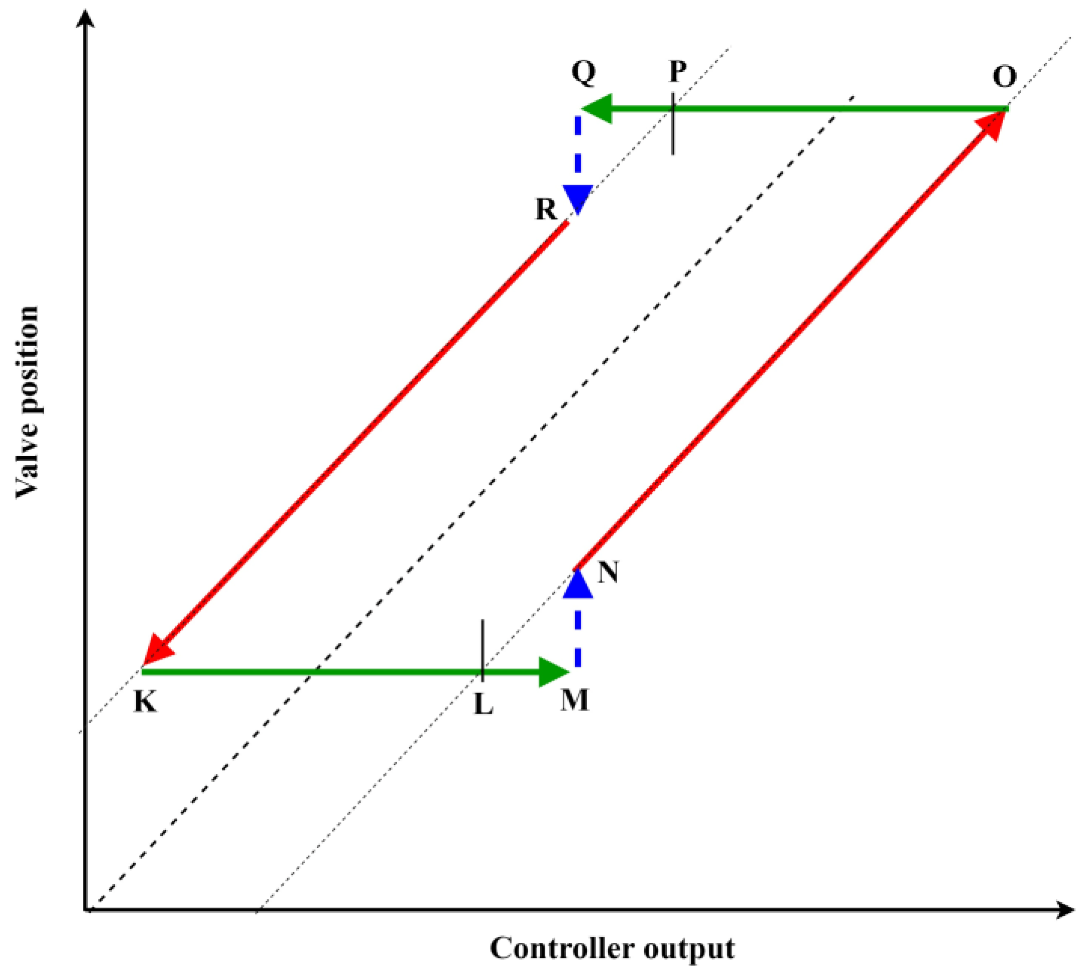
The main cause of static friction or stiction is opposition to the movement of the valve stem. Thus, valve movement is achieved when the pressure applied on the valve to cause movement in the valve stem must overcome the opposing forces obstructing valve movement. When the applied force surpasses the static friction force, a sudden movement in the valve stem can be observed, which is due to the dynamic friction force based on the velocity of the stem movement. Then, because of the velocity, the valve becomes stuck in the new position. The controller starts reducing the input when the actual valve position is more than the required position. Thus, such repeated movements cause stick and slip movements in the valve, representing stiction in the control valve. The stiction behavior of the valve is represented by the following three regions: constant, jump, and movement or motion [34], as shown in Figure 2. The constant is the region where there is a change in controller output, whereas no change is observed in the actual valve position or manipulating variable, represented as region ‘KLM’, where ‘KL’ represents the deadband, whereas ‘LM’ represents the stick band. The jump is the region where a sudden change in the valve stem movement is observed, depicted as ‘MN’. Movement or motion is the third region, where the actual valve keeps moving with a very slight variation in the control input, represented as ‘NO’. This behavior is observed when the controller input continuously increases, and stick jump operations are also observed when the controller output is reduced, as represented by ‘OPQK’. In Figure 2, the green line represents the constant region, the movement of the valve is represented by the red line, and the jump phases are represented by the blue dashed line.
The stiction in a valve is nonlinear, thus exhibiting abnormal behavior that affects the valve behavior slowly. It is one of the incipient faults in pneumatic control valves; thus, the detection of stiction is challenging. For this reason, many researchers have worked in the area of modeling stiction to gain sound knowledge of stiction faults and determine their behavior under various conditions. An empirical model that simulates the stiction behavior for various stick band and jump values was detailed in [35]. The enhanced version of the model specified in [35], also known as the Choudhury stiction model, was reported with the inclusion of other parameters in [36]. Another nonlinear model that considers stiction was reported in [37], in which stiction was also detected. The identification of friction faults using a smoothed model was highlighted in [38], and the use of a data-driven fuzzy system was reported in [39]. Some researchers have added their contributions to the stiction detection domain. A technique for identifying stiction in control valves by calculating the cross-correlation between a control signal and a loop output was described in [40]. The signals shifted because of static friction by approximately π/2, resulting in an odd cross-correlation function.
An even cross-correlation function is produced in the presence of additional disturbances. Therefore, the presence of stiction in control valves is implied by the occurrence of odd cross-correlation functions. This technique was examined utilizing industry statistics regarding oscillation occurrence. Three stiction detection techniques, relay, bicoherence, and cross-correlation, were described in [41] with a comparative inference of better performance on the use of the bicoherence method. The detection of stiction based on the movement of the plot of controller output and valve position was described in [42]. This method is a qualitative approach, and an indicator is used for the detection of stiction. Multiple stiction detection algorithms were utilized in [43], where one of them was selected for the detection of stiction. The methods used were histograms, the area ratio, curve fitting, and cross-correlation, with the inclusion of an index for each method. A study based on various distinctive regions between valve movement and controller output was reported in [44]. The final detection was carried out by observing the regions created by plotting the controller output with the valve position plot. In [45], an approach was used to quantify the deadband, stick band, and slip jump properties of valve stiction by using the special shape created on the Riemannian manifold. A method for detecting stiction by computing the Hurst exponent after the extraction of slow features from the processed controller output and controlled process variable data was reported in [46]. A technique that combines the moving window approach and K-means clustering to identify severe valve stiction or unexpected valve shuts was discussed in [47]. There are some issues in the process of stiction detection in industrial process systems, such as the presence of noise, disturbance, and low sampling, which affect the accuracy of detection [48].
In [49], stiction in control valves was detected based on the Poincaré plot, which is mainly based on correlation in a given time series. These Poincaré plots are given as input to a convolution neural network for training and detecting a stiction fault. A method for the detection of stiction was developed in [50] using a convolution neural network in which the network was trained using time series data. A method for stiction severity identification was reported in [51], where a convolutional neural network was used to detect a stiction fault. The severity is identified by the neural network based on the statistical process control chart generated by principal component analysis.
Our work aims to develop a method for detecting stiction in control valves designed through pattern recognition using an ANN. The discussed method uses the process variable (PV) and controller output (OP) to determine if a control loop suffers from stiction. The data used to train the network are artificially generated using a data-driven model. Two preprocessing techniques, i.e., the D-value method, by calculating the distance between each data point from the centroid, and a feature reduction PCA method, are applied before training the network. The importance of features in stiction detection techniques is the primary objective of this paper. Validation and testing are performed on real industrial data provided by the International Stiction Database (ISDB) [51]. The data-driven model is implemented on SIMULINK, and the ANN is trained on MATLAB using the Pattern Recognition Toolbox.

2. Background Study

Most stiction detection techniques are based on the features of the plot between the controller output and the process variable. To observe the impact of features in stiction detection methods, preprocessing methods, namely, the D-value method and a feature reduction PCA method, are considered. In this section, the introduction to methods used in stiction detection such as data fusion, neural networks, the D-value, and principal component analysis (PCA) are detailed.

2.1. Multisensor Data Fusion

Sensor fusion is a technique that combines data from various sensors to produce information superior to what would be possible from any single sensor. This rapidly growing field is increasingly applied across diverse sectors, including biomedical, aerospace, and environmental systems. The benefits of sensor fusion are manifold, offering deeper analysis, enhanced system resilience, and more precise predictions with reduced uncertainty. Multisensor data fusion, in particular, integrates observations from multiple sensors, both similar and different, to create a more comprehensive and robust depiction of a target environment or process. This approach has recently gained significant traction, with applications in navigation, robotics, and industrial automation, among others. It leverages the redundancy of measurements to improve system robustness and accuracy, leading to better performance of integrated multisensory systems. The fusion process encompasses various related fields, such as signal processing, sensor management, and artificial intelligence techniques.

2.2. Neural Network

Neural networks are learning algorithms used in the machine learning domain. They are vaguely modeled as biological neural networks in animals. A neural network learns to perform tasks by analyzing the example inputs and outputs provided to it. They are predominantly used in pattern recognition applications, and the recognized patterns are represented numerically in a vector.
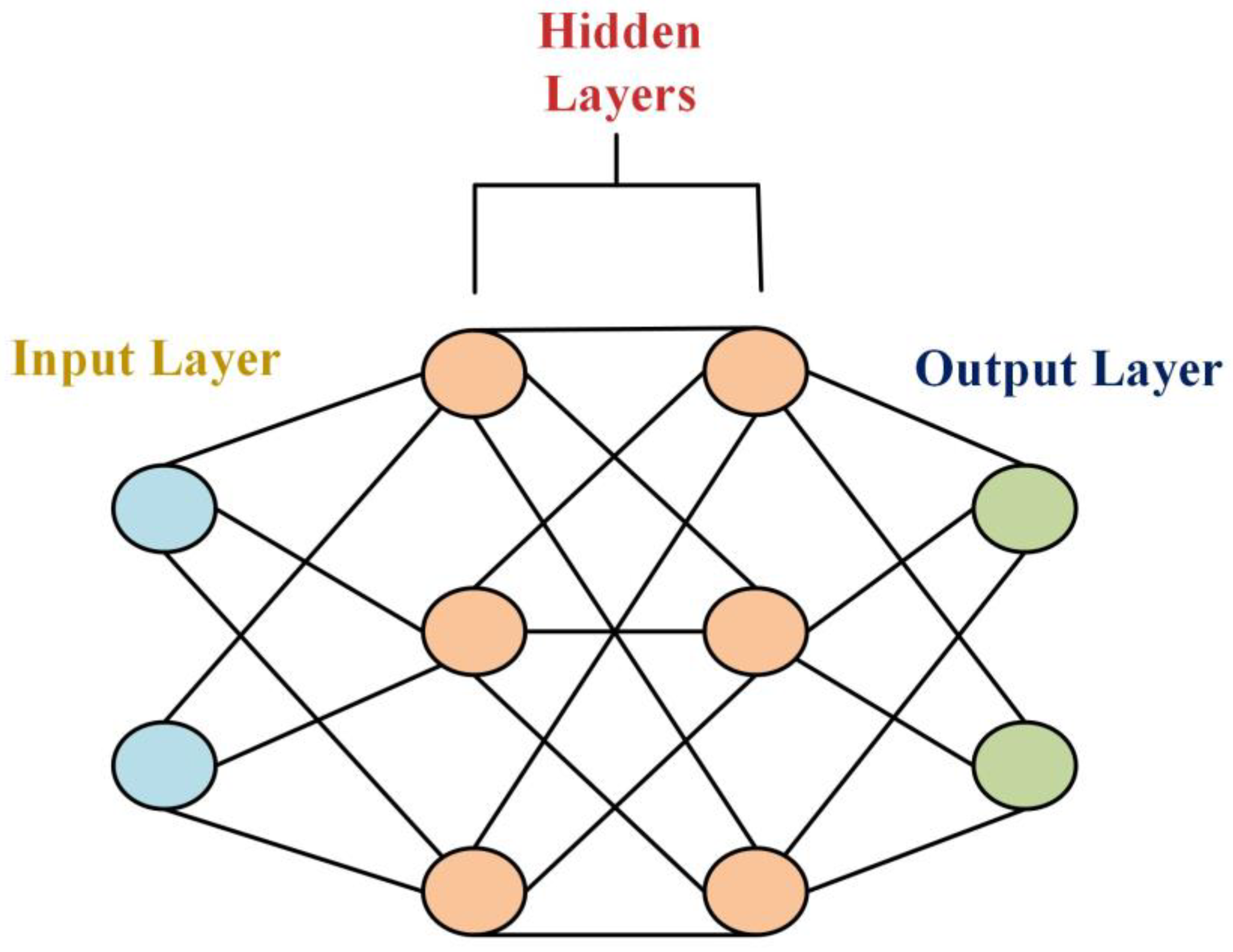
A typical neural network consists of multiple hidden layers with multiple neurons, as shown in Figure 3. The larger the neural network is, the greater the computational cost and time, with or without a significant increase in performance due to phenomena such as overfitting. A neural network learns by adjusting its weights, which is performed by calculating the cost function. The cost function is the difference between the actual and predicted values. The fundamental goal of training a neural network is to minimize this cost function. Based on this calculated cost function, the weights are adjusted. This process of adjusting the weights based on the cost function is called backpropagation.

2.3. D-Value

The D-value is merely a distance and is based on the concept of the centroid. The centroid is the center of mass of the data and is calculated using Equations (1) and (2) on both the x-axis and y-axis for OP and PV, respectively. As discussed in the Introduction, the plot of controller output versus process variable generates a pattern that changes based on the S and J values. Instead of considering the pair of process variable and controller output, calculating the distance of each data point from the centroid reduces the number of input neurons required in the network. Once the centroid of the values in each axis is calculated, the distance of every single data point from the centroid is calculated as represented in Equation (3).
  x c = 1 N i = 1 N x i
y c = 1 N i = 1 N y i
D i = ( x i x c ) 2 + ( y i y c ) 2
where N is the total number of time samples, x i is the i t h OP value, and y i is the i t h PV value.

2.4. PCA

PCA is a prominent dimensionality reduction technique. It distinctly merges the input variable such that only the important or most valuable set of variables is preserved. The new set of variables obtained after performing PCA are bound to be linearly independent of each other and will be the rank order of the variance in each variable (the most important principal axis comes first).
The simplified overall procedure for performing PCA is as follows:
  • Calculate the covariance matrix Σ of the data points.
Σ = 1 m   i = 1 n x ( i ) ( x ( i ) ) T  
where m is the total number of samples and n is the number of dimensions.
2.
Compute the eigenvectors of covariance matrix Σ.
3.
Choose the first k eigenvectors, which are the new k-dimensions.
4.
Transform the original n-dimensional data points into k-dimensions.
  [ n e w   d a t a ] k × 1 = [ t o p   k   e i g e n v e c t o r s ] k × n [ o r i g i n a l   d a t a ] n × 1  
In this work, the Choudhury stiction model is simulated to obtain the open loop response of the stiction behavior. In this paper, two preprocessing methods for training an ANN are compared. Preprocessing the training data enhances the results of a neural network [52]. To emphasize the influence of the preprocessing method on stiction detection, two methods, one with reduction in neural network points without reduction in the features, namely, the D-value method [53], and a feature reduction PCA method of the data, are calculated. These methods are compared for their performance in further sections, and the results emphasize that the feature reduction technique leads to a lowered stiction detection rate.

3. Methodology

This section discusses the approach followed in this work. Fault detection is performed through a pattern recognition neural network. The process of building an artificial neural network for pattern recognition, which includes data processing, training the network, and testing its performance, is examined here.
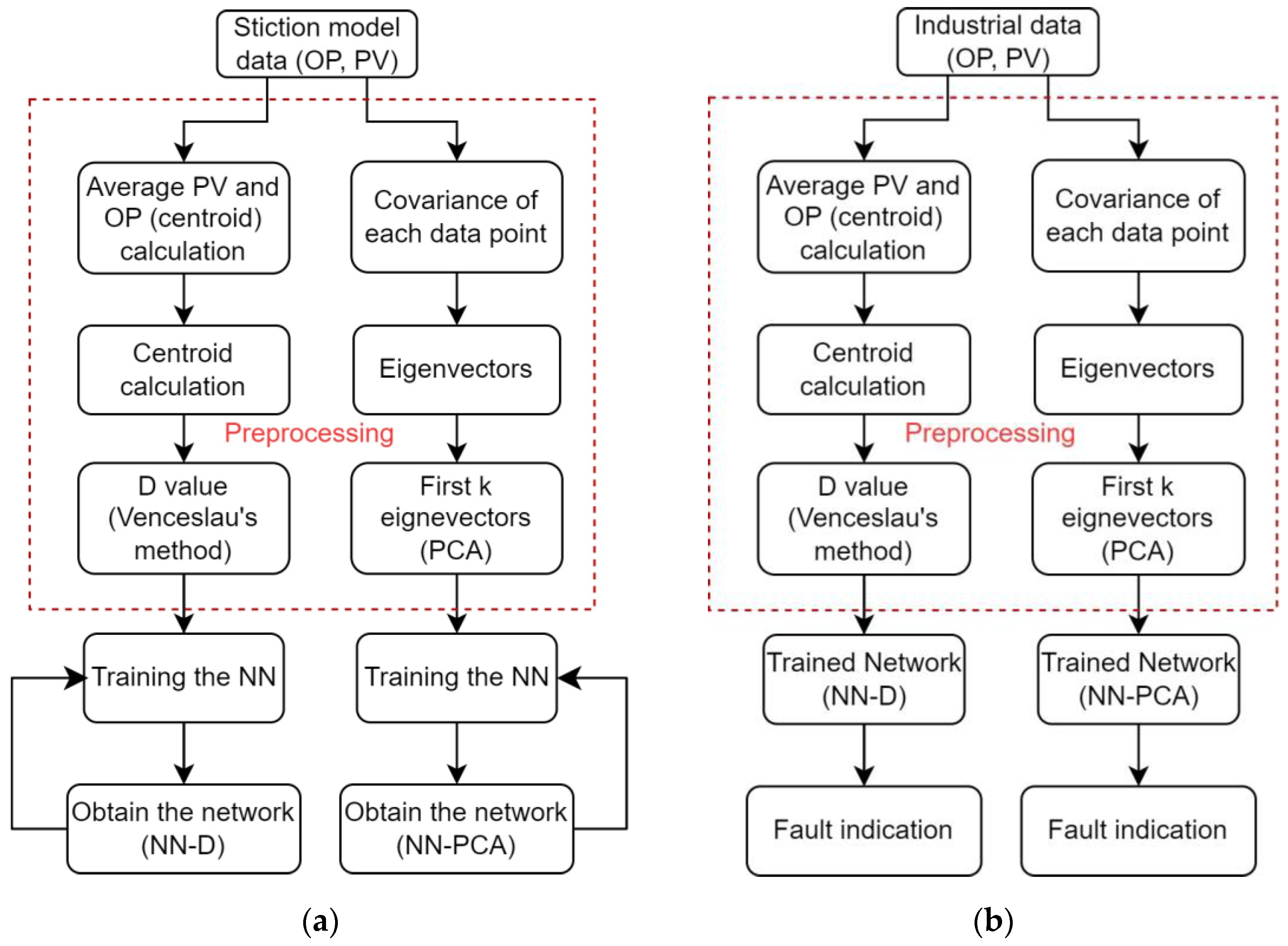
Artificial neural networks have gained significant importance in detection and classification applications because of their ability to perceive data behavior. The performance of ANNs mainly depends on the training methods, the data used for training, and the network structure. To analyze the influence of preprocessing the data utilized for training the network, in this work, two methods of data preprocessing, namely, the D-value method proposed by Venceslau [53] and PCA, are used. Figure 4a shows the steps involved in training the neural network, and Figure 4b shows the steps involved in testing the detection rate of the trained neural network.
In the training process, the simulated stiction data from the Choudhury striction model are generated for various combinations of the deadband plus stick band (S) and slip jump (J) values (represented in Figure 2). These simulated data are then sent to the preprocessing block where the D value and PCA are calculated. These processed data are input to the neural network to train the network. The trained network is then subjected to offline industrial data with and without stiction to test the performance of the networks. A comparison of these methods based on the detection rate is discussed in the Results Section. cata fusion is mainly performed in the preprocessing and training stages of the neural network, as the result mainly depends on the combination of PVs and MVs. In this paper, a comparison of fault detection methods based on two preprocessing methods is carried out.

3.1. Artificial Data Generation

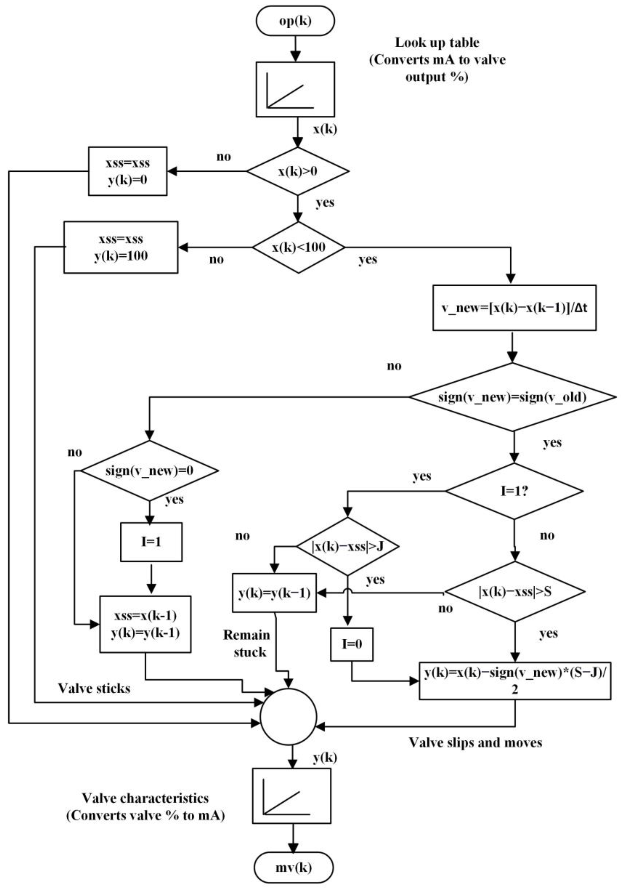
The required data for training the neural network were generated using a Choudhury Stiction data drive model, as shown in Figure 5. It is a data-driven model that has parameters that can be related to plant data, and it produces behavior similar to a physical model. The model only needs the input signal and the specifications of S and J. The stiction model receives the controller’s current output, which ranges from 4 to 20 mA, and converts it to a percentage of valve movement, ranging from 0 to 100%. The valve is said to be fully saturated (i.e., fully open or fully closed) if the valve movement is greater than 100%. The stiction model calculates the slope of the input or control signal when the valve movement lies between 0 and 100%. The model output varies with respect to the sign of the slope of the control signal.
Figure 5 shows the flowchart of the process of generating stiction data. The stiction block input is the control signal x k at 4–20 mA, and the output is the control valve movement y k in terms of the percentage of full-scale movement. For increasing control input, the sign function gives a positive output, whereas it gives a negative output for a decreasing control signal. The sign function returns a ‘0’ when there is no change in the control signal from its previous value; thus, the valve is stuck. If a sign change from positive to negative is observed in the control signal, it represents the start of the stick phase, and the corresponding valve position is considered to be ‘xss’. On observing the change in the sign of the slope, the valve slips and starts moving if the total change in input beats the stick band and/or deadband. This stick–slip action may repeat in the same direction, thus indicating that ‘I’ is ‘1’ for the stick phase and ‘0’ for the jump phase.
The different kinds of stiction that can be obtained based on the values of ‘S’ and ‘J’ are specified below:
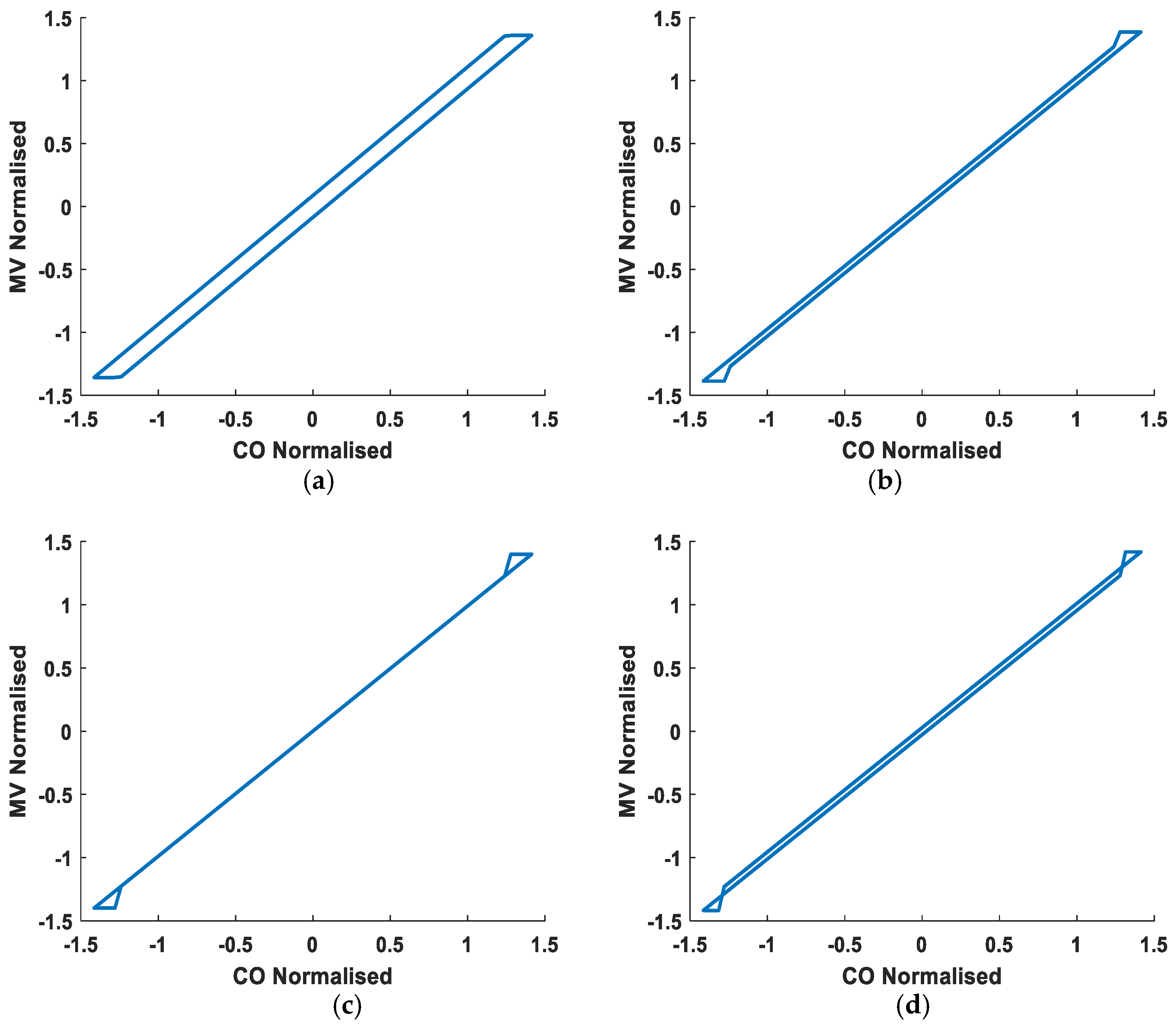
  • Deadband: The response of the controller output to the valve position creates a deadband without any sudden jumps, as this case is simulated when J is a null value, J = 0, as presented in Figure 6a for S = 6.
  • Undershoot: This region is created when the value of ‘J’ is less than the deadband, J < S, as represented in Figure 6b for S = 6 and J = 4.
  • No offset: When the values of ‘S’ and ‘J’ are the same, J = S, this region is created, and it produces pure stick–slip behavior, as shown in Figure 6c for S = J = 6.
  • Overshoot: If the ‘J’ value exceeds the ‘S’ value, J > S; this leads to an overshoot region of stiction as the jump amplitude is greater than the deadband, as depicted in Figure 6d for S = 4 and J = 6.
The Choudhury stiction model depicted in Figure 5 was implemented in SIMULINK and MATLAB. The open loop stiction behavior was analyzed by applying a sinusoidal control input to the stiction model to simulate the stiction behavior of the valve. The obtained valve position was plotted with the controller output for various combinations of ‘S’ and ‘J’ values, as represented in Figure 6. To analyze the response of the flow process for the stiction fault, a flow process model G(S) was considered and placed in series with the plant model. The flow process model G(S) considered for this study is given in Equation (6) [54].
G S = 0.615   20 s + 1 e 10 s  
Using the Choudhury model, open loop data were generated for stiction behavior for various combinations of ‘S’ and ‘J’ values [55]. The responses shown in Figure 6 are from an open-loop system where the input is a sine wave with an amplitude of 50 and a frequency of 0.02 π rad/s. The responses obtained were normalized before plotting the controller output versus the valve stem movement. The output was calculated using the following equation:
y k = x k s i g n s l o p e × ( S J ) / 2  
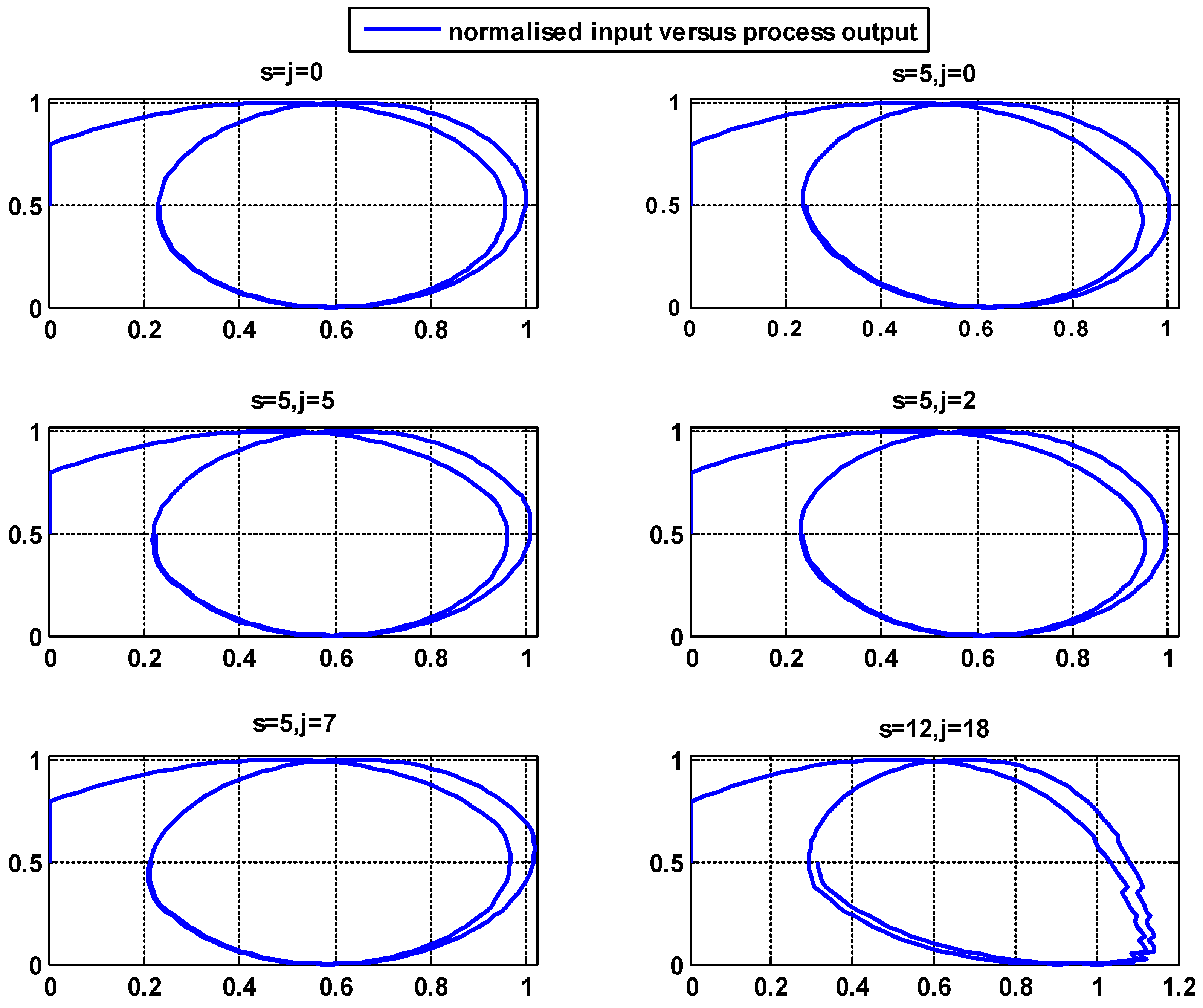
When the flow process model given in Equation (6) was placed in series with the stiction model, the closed-loop response of the flow model with stiction is represented in Figure 7. The process outputs were obtained for 6 different combinations of ‘S’ and ‘J’ values, and the process output versus input is plotted in Figure 7. The graph shows that by varying the values of ‘S’ and ‘J’, the shape of the input versus the output is slightly varied in terms of the orientation and amplitude of these graphs. Both the controller output and manipulating variables were normalized and then plotted to obtain their relationships.
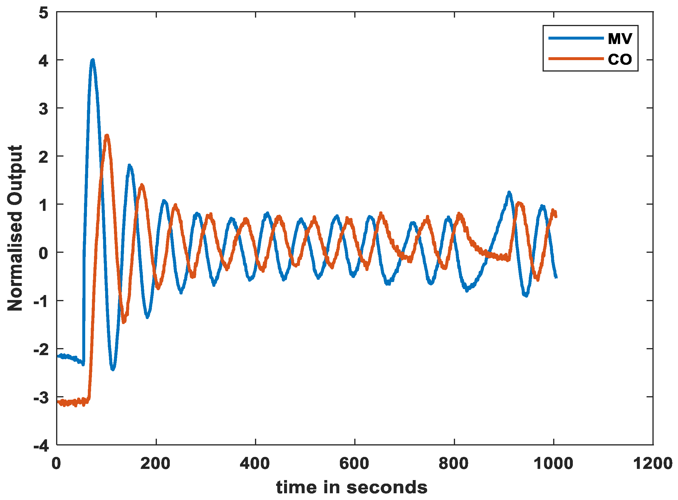
Gaussian-distributed white noise with zero means was also added so that the training data resembled the practical outputs. As the open loop system was considered, the controller output in the form of a sinusoidal wave was given to the process. Based on this model, the data necessary to train the neural network were obtained. The generated dataset responded with and without stiction by varying the S and J parameters.
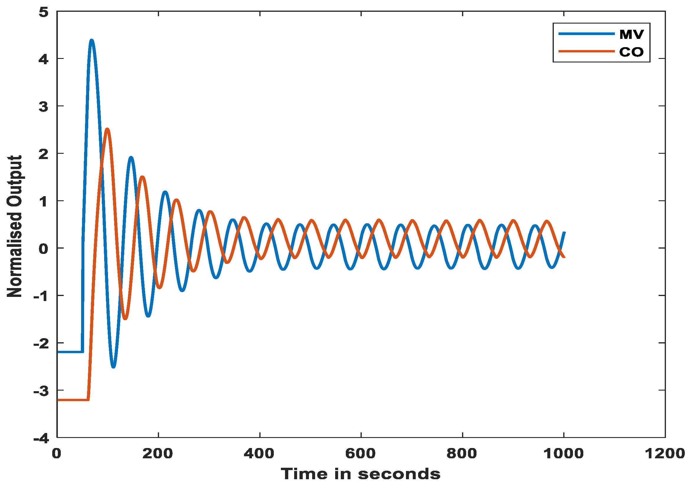
The generated stiction data were based on the combination of S and J values, as shown in Table 1. The closed-loop response of the system is shown in Figure 8. Oscillations due to the stiction parameters S and J are noticeable in this system. The response of the same system to Gaussian-distributed white noise is shown in Figure 9. A total of 13,388 datasets consisting of PV and OP were created, of which 8000 were stiction samples and 5388 were without stiction. Not all the data generated were used to train the neural network. The parameters used for generating the dataset are shown in Table 1 [4].
The variance for the Gaussian distribution was set to a random value between 0.01 and 0.2. The data generated without stiction were based on the combination of the K p and K I values of the proportional–integral (PI) controller, as shown in Table 2, which generates the response of a well-tuned PI controller and an excessively tuned PI controller. Additionally, data were generated for a well-tuned PI with an external disturbance, which was applied in the form of a sine wave. The range of the sine wave generator is shown in Table 3.

3.2. Data Preprocessing

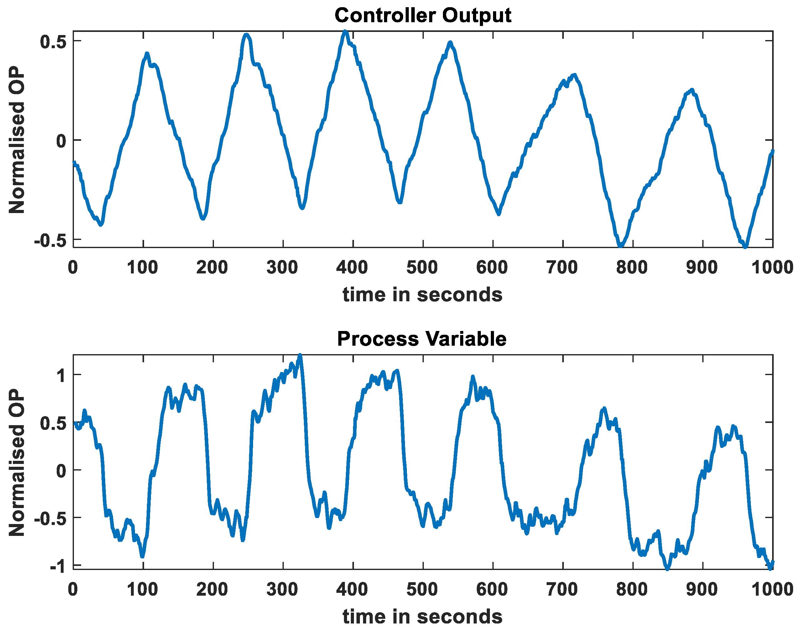
Before the neural network was trained, data preprocessing was performed. From the generated data, a window of precisely 500 discrete-time signals of both the PV and OP was selected. To train the artificial neural network, the values of PV and OP of the N time stamp were needed. Therefore, if both PV and OP were considered, and an output with 2 N time samples was produced in total. This can increase the training period and can take up a large amount of memory. Therefore, to reduce the total number of time samples, dimensionality reduction must be performed. This paper considers two methods, D-values and PCA, and their respective performances are discussed in the Results Section. The original process variable and controller output of a control loop (CHEM 1 of ISDB) are shown in Figure 10.
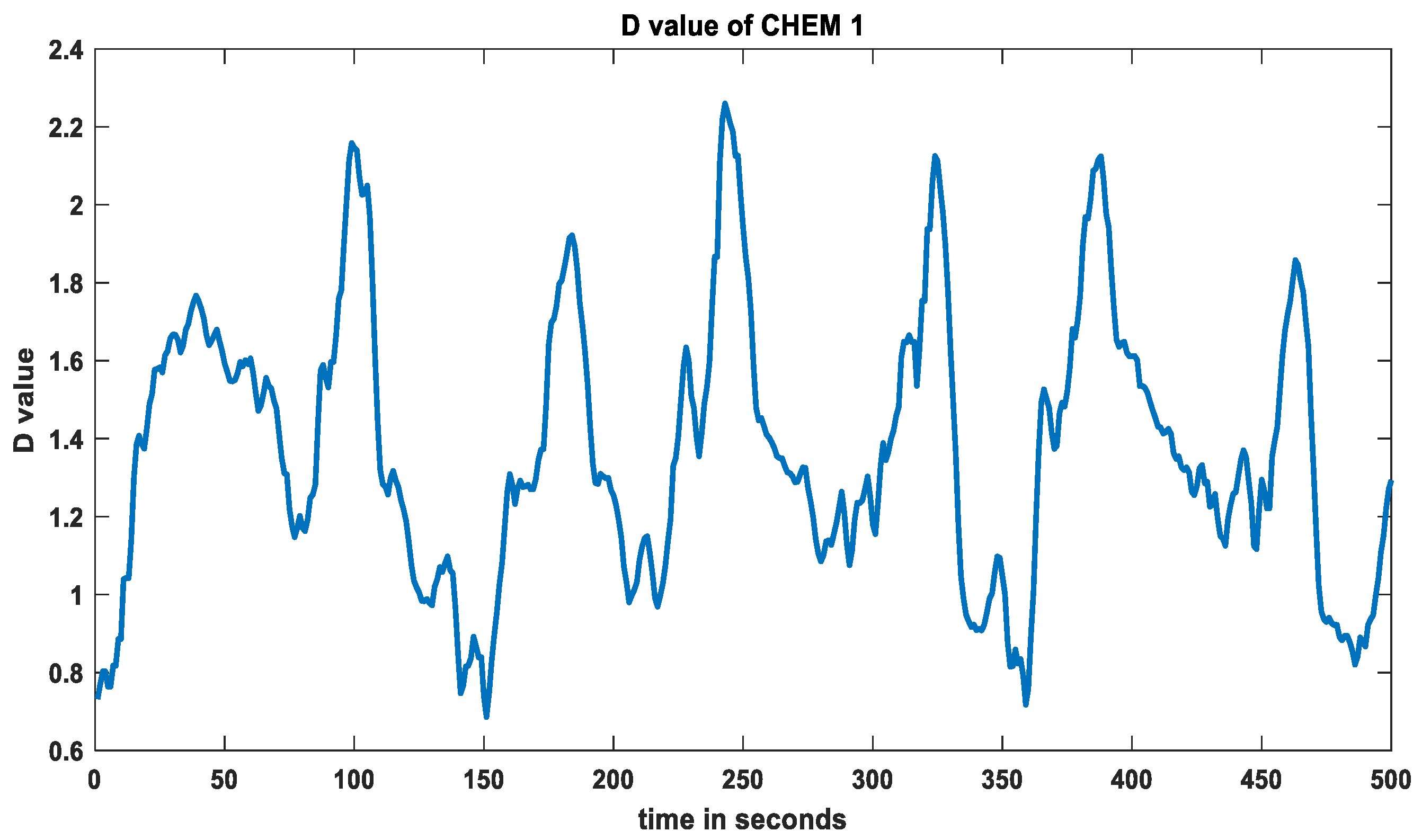
D-values for the first 500 timestamps of CHEM loop 1 were collected and then normalized based on range, as shown in Figure 11. D-values for different samples were then calculated and used to train the neural network.
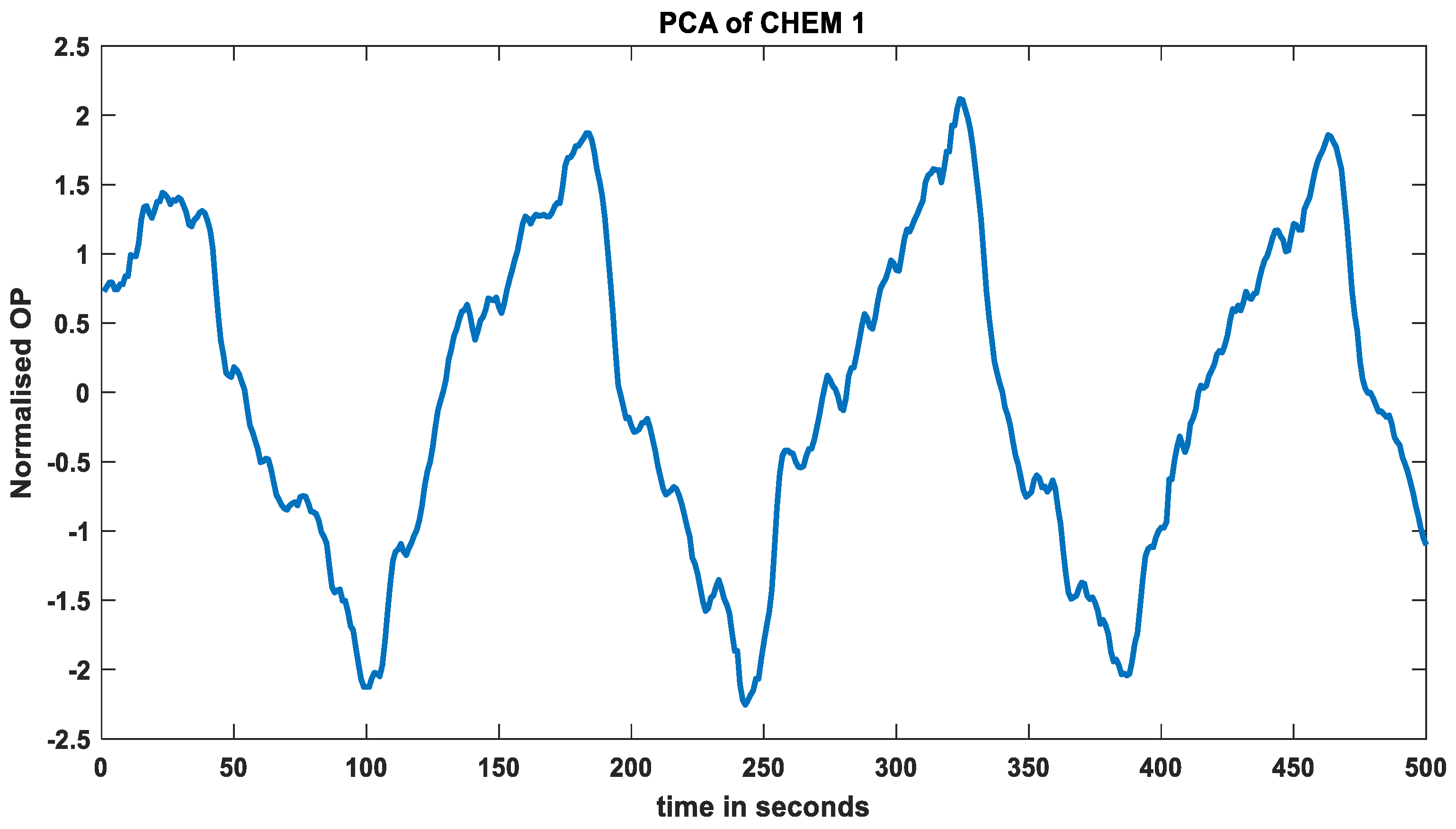
PCA values for the first 500 timestamps were collected for CHEM loop 1 and then normalized based on the range, as shown in Figure 12.

3.3. NN Architecture

The proposed ANN consists of 4 layers, the input layer, two hidden layers, and the output layer. The input layer consists of 500 neurons for 500 timestamps. The hidden layer consists of 10 neurons each. The output layer with two neurons indicates [1; 0] for the presence of stiction and [0; 1] for no stiction. Both hidden layers use the tan-h activation function, and the training method used is scaled conjugate gradient backpropagation.
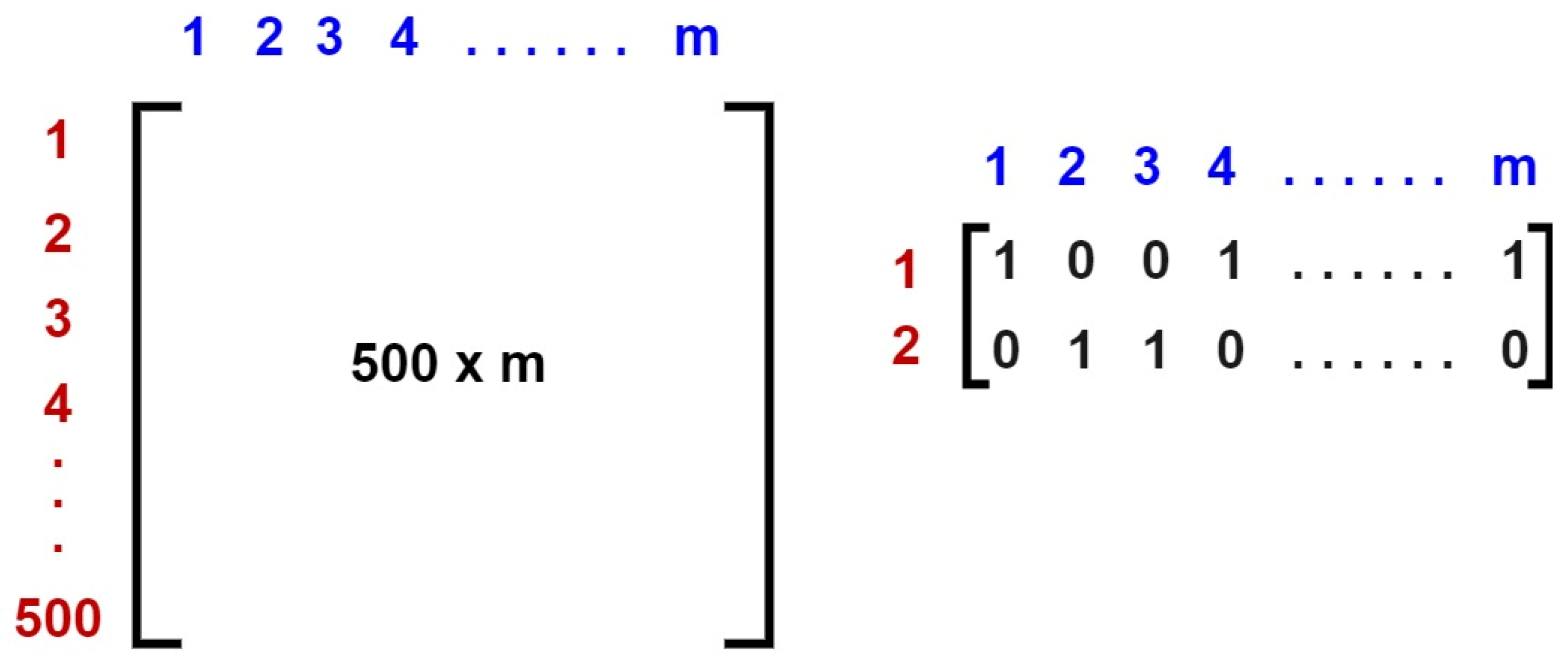
The training input (D-value or PCA value) and its corresponding output, which indicate the presence of stiction, are represented in matrix form, as shown in Figure 13. Here, ‘m’ is the total number of training samples used. Once the neural network was trained, the network was validated and tested using the ISDB dataset. Since the classification of the stiction of these datasets was known, a quantitative analysis of the trained neural networks could be performed. A comparison of the two preprocessing methods for a variety of training algorithms is discussed in the next section.

4. Results and Discussion

In this section, the criteria through which the neural networks were optimized are demonstrated along with the performance of two data preprocessing methods. The D-value and PCA were computed as discussed in the previous section. An example of performing these methods on the CHEM 1 loop of ISDB data is shown in Figure 9 and Figure 10. Interestingly, when all the generated data were used, the ability of the network to detect nonstiction data wasc considerably low. This indicated that samples from different sources were highly similar between the stiction and nonstiction groups. Since overfitting of the stiction data was present, the prediction accuracy of the individual noise level was tested, as shown in Table 4.
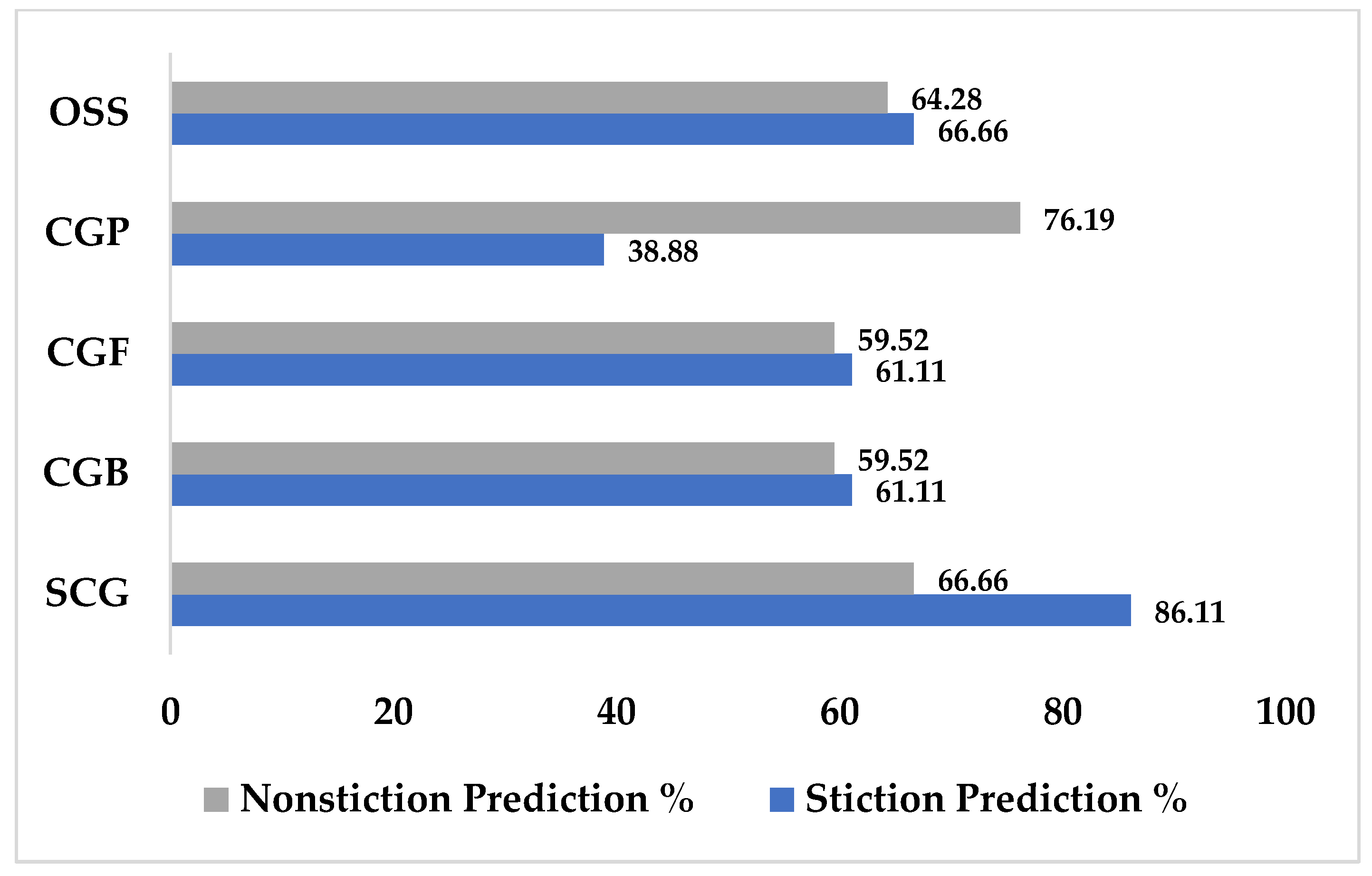
Table 4 shows that using only the noise level with a variance of 0.040.5 gave the best result, followed by a variance of 0.050.5. Surprisingly, when noise with both of these variances was combined, an accuracy of 76.38% was obtained. Once the dataset used to train the neural network was determined, the performances of the different training algorithms were analyzed. The results are shown in Table 5. The scaled conjugate gradient was found to yield the highest accuracy for the detection of stiction. Even though a total performance of 76.28% was achieved, the ability of the network to accurately detect nonstiction loops did not reach the mark. Although stiction detection had a prediction accuracy of 86.11%, the nonstiction prediction accuracy was only 66.66%. A comparison of the results obtained using the different learning algorithms mentioned in Table 5 is shown in Figure 14.
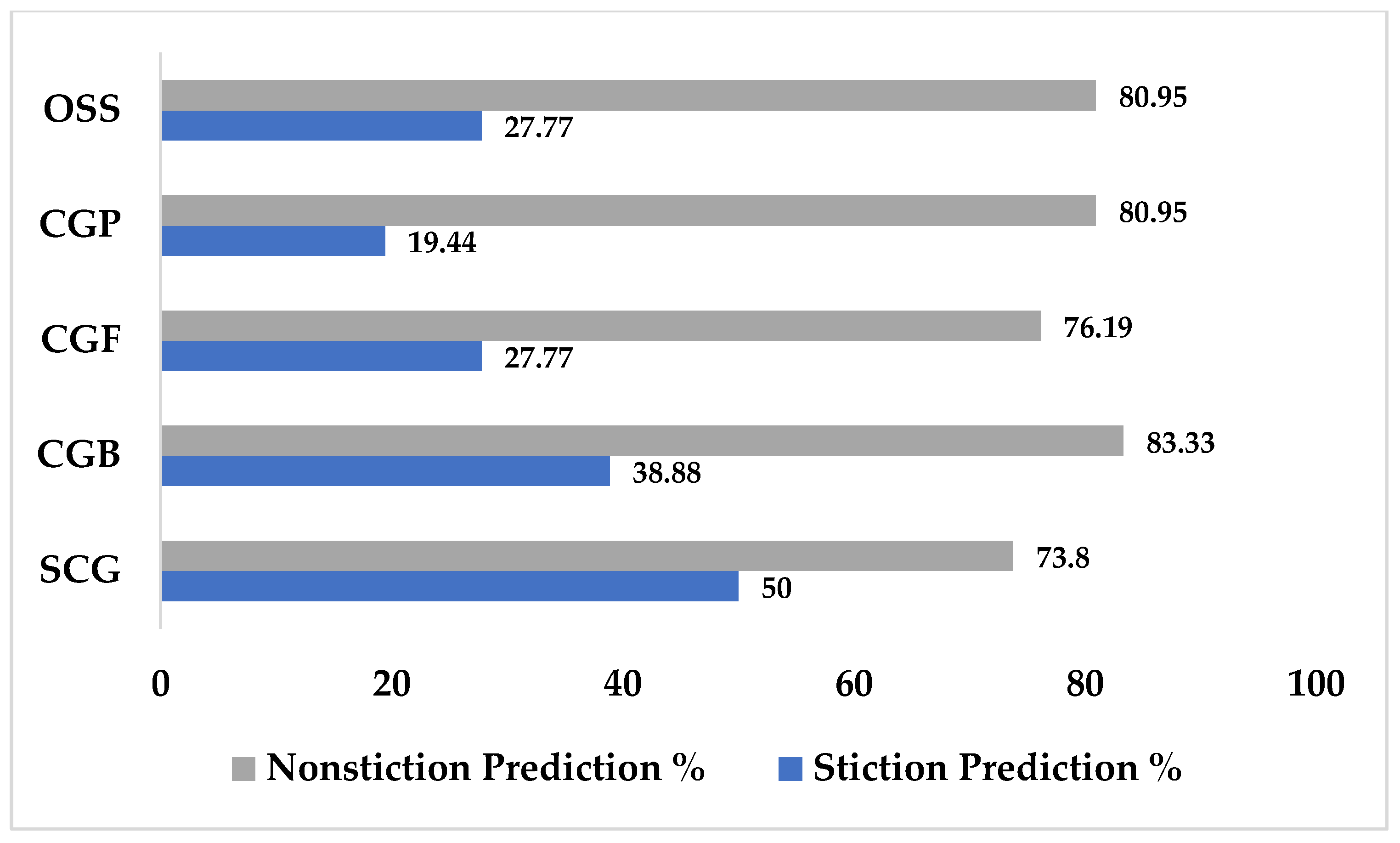
A similar test was also performed on the data that were reduced by PCA to determine which learning algorithm and set of training data yielded the highest results. Through this test, it was found that the combination of datasets involving variances of 0.010.5, 0.040.5, and 0.050.5 gave the best results. By comparing their performances to those of the learning algorithms, a similar prediction in terms of accuracy was achieved when using SCG or the conjugate gradient with Powell/Beale restart (CGB), as shown in Table 6. Although their overall prediction accuracies were similar, the abilities of both methods to detect stiction and nonstiction loops were different. While SCG had a prediction accuracy of 50%, CGB achieved even worse results, with a performance of 38.88%. However, the nonstiction prediction performance of CBG was higher than that of SCG, with the former having a prediction accuracy of 83.33% and the latter having a prediction accuracy of 73.80%, as shown in Figure 15.
A neural network that can identify stiction in control valves was designed and tested on a real industrial benchmark control loop to verify the validity of the network. The data used to train the network were obtained artificially using a data-driven Choudhury’s stiction model. The model used two variables, S and J, to model the network. The data obtained from these data were used to train the neural network. The generated neural network was based on two preprocessing methods, namely, D-values and PCA. On comparing these preprocessing methods, the D-value method achieved a better accuracy of 73.4% for a noise variance of 0.04. Thus, reducing the number of features reduces the prediction accuracy. Validation and testing of the neural network were performed on the industrial loop CHEM loop1 from ISDB data.

5. Conclusions

The comparative study presented in this paper demonstrates the effectiveness of preprocessing methods for detecting stiction in industrial control valves using ANN based on pattern recognition. By leveraging PVs and OPs, the D-value method accurately identifies stiction within control loops. The ANN, trained with preprocessed data from a robust data-driven model through the application of two methods, namely, the D-value and PCA, was validated and tested with real industrial data from the ISDB.
This study’s evaluation of two preprocessing methods revealed a significant impact on fault detection accuracy, with an overall accuracy of 76%, an 86% precision rate in stiction prediction, and a 66% success rate in nonstiction scenarios when using D-value preprocessing. This indicates that the pattern between PV and OP is crucial in detecting the stiction fault. Implementing the data-driven model in SIMULINK and training the ANN in MATLAB with the Pattern Recognition Toolbox underscore the practical application and reliability of the method.
These promising results indicate that the fault detection technique with D-value preprocessing can reliably diagnose stiction in industrial settings, offering a valuable tool for enhancing maintenance protocols, reducing operational downtime, and improving overall efficiency. Future research will focus on broadening the method’s applicability to a diverse range of control systems and operational conditions, further solidifying its value in industrial practices. Integrating this technique into existing control systems is anticipated to drive significant improvements in system performance and reliability. It is evident from the performed experiment that using the D-value for data processing yields better prediction accuracy than PCA. This is because the D-value, which is based on the centroid principle, is better at representing stiction properties than PCA, which is based on the covariance of variables.
Sensor fusion is the ultimate form of sensor integration. By reducing the computational complexity and size to increase the accuracy, reliability, and performance, sensor fusion has been adopted in many industries to generate better outputs. The added layer of redundancy always benefits the clarity of the result and its error diagnosis.
Through sensor fusion applications, as we briefed about in this paper, complex fault identification, classification, and diagnosis tasks are made more straightforward. Correlating them with most modern technology innovations such as neural networks and machine learning has become a breakthrough in the quality control process.

Author Contributions

Conceptualization, S.K.V. and B.R.N.; methodology, B.R.N., S.K.V. and V.S.; software, B.R.N.; validation, B.R.N. and S.K.V.; formal analysis, V.S.; investigation, B.R.N.; writing—original draft preparation, B.R.N., V.S. and S.K.V.; writing—review and editing, S.K.V.; supervision, S.K.V.; project administration, S.K.V. All authors have read and agreed to the published version of the manuscript.

Funding

This research received no external funding.

Data Availability Statement

The original contributions presented in the study are included in the article, further inquiries can be directed to the corresponding author.

Conflicts of Interest

The authors declare no conflicts of interest.

References

  1. Valette, E.; El-Haouzi, H.B.; Demesure, G. Industry 5.0 and its technologies: A systematic literature review upon the human place into IoT-and CPS-based industrial systems. Comput. Ind. Eng. 2023, 184, 109426. [Google Scholar] [CrossRef]
  2. Wolfe, M.T.; Patel, P.C. Same difference? The impact of low-, medium-, and high-tech industries on venture performance and survival. IEEE Trans. Eng. Manag. 2019, 68, 1907–1918. [Google Scholar] [CrossRef]
  3. Wang, Z.; Fan, Y. Monitoring-performance-indicator-related industrial process monitoring with a monitoring index identification model. Control Eng. Pract. 2023, 139, 105660. [Google Scholar] [CrossRef]
  4. Asrol, M.; Wahyudi, S.; Harito, C.; Utama, D.N.; Syafrudin, M. Improving Supplier Evaluation Model using Ensemble Method-Machine Learning for Food Industry. Procedia Comput. Sci. 2023, 227, 307–315. [Google Scholar] [CrossRef]
  5. LaNasa, P.J.; Upp, E.L. Fluid Flow Measurement: A Practical Guide to Accurate Flow Measurement; Butterworth-Heinemann: Oxford, UK, 2014; pp. 35–47. [Google Scholar]
  6. Elijah, O.; Ling, P.A.; Rahim, S.K.A.; Geok, T.K.; Arsad, A.; Kadir, E.A.; Abdurrahman, M.; Junin, R.; Agi, A.; Abdulfatah, M.Y. A survey on industry 4.0 for the oil and gas industry: Upstream sector. IEEE Access 2021, 9, 144438–144468. [Google Scholar] [CrossRef]
  7. Liu, J.; An, R.; Xiao, R.; Yang, Y.; Wang, G.; Wang, Q. Implications from substance flow analysis, supply chain and supplier’risk evaluation in iron and steel industry in Mainland China. Resour. Policy 2017, 51, 272–282. [Google Scholar] [CrossRef]
  8. Jia, Y.; Zhang, Z.G.; Xu, T. Improving the Performance of MMPP/M/C Queue by Convex Optimization–A Real-World Application in Iron and Steel Industry. IEEE Access 2020, 8, 185909–185918. [Google Scholar] [CrossRef]
  9. Xiao, H.; McDonald, D.; Fan, Y.; Umbanhowar, P.B.; Ottino, J.M.; Lueptow, R.M. Controlling granular segregation using modulated flow. Powder Technol. 2017, 312, 360–368. [Google Scholar] [CrossRef]
  10. Nawaz, M.; Maulud, A.S.; Zabiri, H.; Suleman, H. Review of multiscale methods for process monitoring, with an emphasis on applications in chemical process systems. IEEE Access 2022, 10, 49708–49724. [Google Scholar] [CrossRef]
  11. Shah, R.B.; Tawakkul, M.A.; Khan, M.A. Comparative evaluation of flow for pharmaceutical powders and granules. Aaps Pharmscitech 2008, 9, 250–258. [Google Scholar] [CrossRef]
  12. Wang, Z.; Tang, S.; Guo, G.; Yang, Y.; He, D.; Yang, L.; Han, M.; Hou, Y. Adaptive Quality Control with Uncertainty for a Pharmaceutical Cyber-Physical System Based on Data and Knowledge Integration. IEEE Trans. Ind. Inform. 2024, 20, 3339–3350. [Google Scholar] [CrossRef]
  13. Bugallo, P.M.B.; Stupak, A.; Andrade, L.C.; López, R.T. Material Flow Analysis in a cooked mussel processing industry. J. Food Eng. 2012, 113, 100–117. [Google Scholar] [CrossRef]
  14. Alves, N.N.; Messaoud, G.B.; Desobry, S.; Costa, J.M.C.; Rodrigues, S. Effect of drying technique and feed flow rate on bacterial survival and physicochemical properties of a nondairy fermented probiotic juice powder. J. Food Eng. 2016, 189, 45–54. [Google Scholar] [CrossRef]
  15. Hawashin, D.; Salah, K.; Jayaraman, R.; Musamih, A. Using Composable NFTs for Trading and Managing Expensive Packaged Products in the Food Industry. IEEE Access 2023, 11, 10587–10603. [Google Scholar] [CrossRef]
  16. Odunlami, O.A.; Amoo, T.E.; Adisa, H.A.; Elehinafe, F.B.; Oladimeji, T.E. Application of mass transfer in the pulp and paper Industry− overview, processing, challenges, and prospects. Results Eng. 2023, 20, 101498. [Google Scholar] [CrossRef]
  17. Liu, Z.; Zhao, L.; Lu, S.; Hou, X.; Hou, D.; Ma, J. Porous ceramsite catalytic ozonation for the treatment of pulp and paper mill wastewater in a continuous-flow reactor. Chem. Eng. Sci. 2024, 288, 119855. [Google Scholar] [CrossRef]
  18. Liu, W.; Hu, J.; Zhao, X.; Pan, H.; Lakhiar, I.A.; Wang, W. Development and experimental analysis of an intelligent sensor for monitoring seed flow rate based on a seed flow reconstruction technique. Comput. Electron. Agric. 2019, 164, 104899. [Google Scholar] [CrossRef]
  19. He, F.; Ma, X.; Shen, K.; Wang, C. Study on material and energy flow in steel forging production process. IEEE Access 2019, 8, 12921–12932. [Google Scholar] [CrossRef]
  20. Navada, B.R.; Santhosh, K.V. Is fault detection and diagnosis in pneumatic actuator a topic of concern? J. Adv. Res. Fluid Mech. Therm. Sci. 2021, 77, 102–129. [Google Scholar] [CrossRef]
  21. Ji, H.; He, X.; Shang, J.; Zhou, D. Incipient fault detection with smoothing techniques in statistical process monitoring. Control Eng. Pract. 2017, 62, 11–21. [Google Scholar] [CrossRef]
  22. Zhang, S.; Luo, M.; Qian, H.; Liu, L.; Yang, H.; Zhang, Y.; Liu, X.; Xie, Z.; Yang, L.; Zhang, W. A review of valve health diagnosis and assessment: Insights for intelligence maintenance of natural gas pipeline valves in China. Eng. Fail. Anal. 2023, 153, 107581. [Google Scholar] [CrossRef]
  23. Shi, J.; Yi, J.; Ren, Y.; Li, Y.; Zhong, Q.; Tang, H.; Chen, L. Fault diagnosis in a hydraulic directional valve using a two-stage multi-sensor information fusion. Measurement 2021, 179, 109460. [Google Scholar] [CrossRef]
  24. Ji, X.; Ren, Y.; Tang, H.; Shi, C.; Xiang, J. An intelligent fault diagnosis approach based on Dempster-Shafer theory for hydraulic valves. Measurement 2020, 165, 108129. [Google Scholar] [CrossRef]
  25. Ma, D.; Liu, Z.; Gao, Q.; Huang, T. Fault diagnosis of a solenoid valve based on multi-feature fusion. Appl. Sci. 2022, 12, 5904. [Google Scholar] [CrossRef]
  26. Ttito Ugarte, L.; Bernardini, F. An Overview on the Use of Machine Learning Algorithms for Identifying Anomalies in Industrial Valves. In World Conference on Information Systems and Technologies; Springer Nature: Cham, Switzerland, 2024; pp. 3–12. [Google Scholar]
  27. Andrade, A.; Lopes, K.; Lima, B.; Maitelli, A. Development of a methodology using artificial neural network in the detection and diagnosis of faults for pneumatic control valves. Sensors 2021, 21, 853. [Google Scholar] [CrossRef]
  28. Sun, F.; Xu, H.; Zhao, Y.H.; Zhang, Y.D. Data-driven fault diagnosis of control valve with missing data based on modeling and deep residual shrinkage network. J. Zhejiang Univ. Sci. A 2022, 23, 303–313. [Google Scholar] [CrossRef]
  29. Jo, S.H.; Seo, B.; Oh, H.; Youn, B.D.; Lee, D. Model-based fault detection method for coil burnout in solenoid valves subjected to dynamic thermal loading. IEEE Access 2020, 8, 70387–70400. [Google Scholar] [CrossRef]
  30. Han, X.; Jiang, J.; Xu, A.; Huang, X.; Pei, C.; Sun, Y. Fault detection of pneumatic control valves based on canonical variate analysis. IEEE Sens. J. 2021, 21, 13603–13615. [Google Scholar] [CrossRef]
  31. An, Z.; Cheng, L.; Guo, Y.; Ren, M.; Feng, W.; Sun, B.; Ling, J.; Chen, H.; Chen, W.; Luo, Y.; et al. A novel principal component analysis-informer model for fault prediction of nuclear valves. Machines 2022, 10, 240. [Google Scholar] [CrossRef]
  32. Durand, H.; Parker, R.; Alanqar, A.; Christofides, P.D. Elucidating and handling effects of valve-induced nonlinearities in industrial feedback control loops. Comput. Chem. Eng. 2018, 116, 156–175. [Google Scholar] [CrossRef]
  33. Brasio, A.S.; Romanenko, A.; Fernandes, N.C. Modeling, detection and quantification, and compensation of stiction in control loops: The state of the art. Ind. Eng. Chem. Res. 2014, 53, 15020–15040. [Google Scholar] [CrossRef]
  34. Daneshwar, M.A.; Noh, N.M. Detection of stiction in flow control loops based on fuzzy clustering. Control Eng. Pract. 2015, 39, 23–34. [Google Scholar] [CrossRef]
  35. Choudhury, M.S.; Thornhill, N.F.; Shah, S.L. Modeling valve stiction. Control Eng. Pract. 2005, 13, 641–658. [Google Scholar] [CrossRef]
  36. Xie, L.; Cong, Y.; Horch, A. An improved valve stiction simulation model based on ISA standard tests. Control Eng. Pract. 2013, 21, 1359–1368. [Google Scholar] [CrossRef]
  37. di Capaci, R.B.; Scali, C.; Pannocchia, G. System identification applied to stiction quantification in industrial control loops: A comparative study. J. Process Control 2016, 46, 11–23. [Google Scholar] [CrossRef]
  38. di Capaci, R.B.; Vaccari, M.; Pannocchia, G.; Scali, C. Identification and estimation of valve stiction by the use of a smoothed model. IFAC-PapersOnLine 2018, 51, 684–689. [Google Scholar] [CrossRef]
  39. Daneshwar, M.A.; Noh, N.M. Identification of a process with control valve stiction using a fuzzy system: A data-driven approach. J. Process Control 2014, 24, 249–260. [Google Scholar] [CrossRef]
  40. Horch, A. A simple method for detection of stiction in control valves. Control Eng. Pract. 1999, 7, 1221–1231. [Google Scholar] [CrossRef]
  41. Rossi, M.; Scali, C. A comparison of techniques for automatic detection of stiction: Simulation and application to industrial data. J. Process Control 2005, 15, 505–514. [Google Scholar] [CrossRef]
  42. Yamashita, Y. An automatic method for detection of valve stiction in process control loops. Control Eng. Pract. 2006, 14, 503–510. [Google Scholar] [CrossRef]
  43. Zakharov, A.; Zattoni, E.; Xie, L.; Garcia, O.P.; Jämsä-Jounela, S.L. An autonomous valve stiction detection system based on data characterization. Control Eng. Pract. 2013, 21, 1507–1518. [Google Scholar] [CrossRef]
  44. Maruta, H.; Kano, M.; Kugemoto, H.; Shimizu, K. Modeling and detection of stiction in pneumatic control valve. Trans. Soc. Instrum. Control Eng. 2004, 40, 825–833. [Google Scholar] [CrossRef]
  45. Kok, T.L.; Aldrich, C.; Zabiri, H.; Taqvi, S.A.A.; Olivier, J. Application of unthresholded recurrence plots and texture analysis for industrial loops with faulty valves. Soft Comput. 2022, 26, 10477–10492. [Google Scholar] [CrossRef]
  46. Shang, L.; Zhang, Y.; Zhang, H. Valve Stiction Detection Method Based on Dynamic Slow Feature Analysis and Hurst Exponent. Processes 2023, 11, 1913. [Google Scholar] [CrossRef]
  47. Zheng, D.; Sun, X.; Damarla, S.K.; Shah, A.; Amalraj, J.; Huang, B. Valve stiction detection and quantification using a k-means clustering based moving window approach. Ind. Eng. Chem. Res. 2021, 60, 2563–2577. [Google Scholar] [CrossRef]
  48. Dambros, J.W.; Farenzena, M.; Trierweiler, J.O. Stiction detection in low sampling rate signals. Can. J. Chem. Eng. 2018, 96, 1735–1745. [Google Scholar] [CrossRef]
  49. Bounoua, W.; Aftab, M.F.; Omlin, C.W.P. Stiction detection in industrial control valves using Poincaré plot-based convolutional neural networks. IFAC-PapersOnLine 2023, 56, 11687–11692. [Google Scholar] [CrossRef]
  50. Zhang, K.; Liu, Y.; Gu, Y.; Ruan, X.; Wang, J. Multiple-timescale feature learning strategy for valve stiction detection based on convolutional neural network. IEEE/ASME Trans. Mechatron. 2021, 27, 1478–1488. [Google Scholar] [CrossRef]
  51. Henry, Y.Y.S.; Aldrich, C.; Zabiri, H. Detection and severity identification of control valve stiction in industrial loops using integrated partially retrained CNN-PCA frameworks. Chemom. Intell. Lab. Syst. 2020, 206, 104143. [Google Scholar] [CrossRef]
  52. Amiruddin, A.A.A.M.; Zabiri, H.; Jeremiah, S.S.; Teh, W.K.; Kamaruddin, B. Valve stiction detection through improved pattern recognition using neural networks. Control Eng. Pract. 2019, 90, 63–84. [Google Scholar] [CrossRef]
  53. Venceslau, A.R.; Guedes, L.A.; Silva, D.R. Artificial neural network approach for detection and diagnosis of valve stiction. In Proceedings of the 2012 IEEE 17th International Conference on Emerging Technologies & Factory Automation (ETFA 2012), Kraków, Poland, 17–21 September 2012; IEEE: New York, NY, USA, 2012; pp. 1–4. [Google Scholar]
  54. Navada, B.R.; Venkata, S. Fusion-based online identification technique for pneumatic actuator faults. Eng. Sci. 2021, 17, 56–69. [Google Scholar] [CrossRef]
  55. Navada, B.R.; Santhosh, K.V. Analysis of Stiction Fault in Pneumatic Control Valves. In Advances in Control Instrumentation Systems: Select Proceedings of CISCON; Springer: Singapore, 2019; pp. 215–226. [Google Scholar]
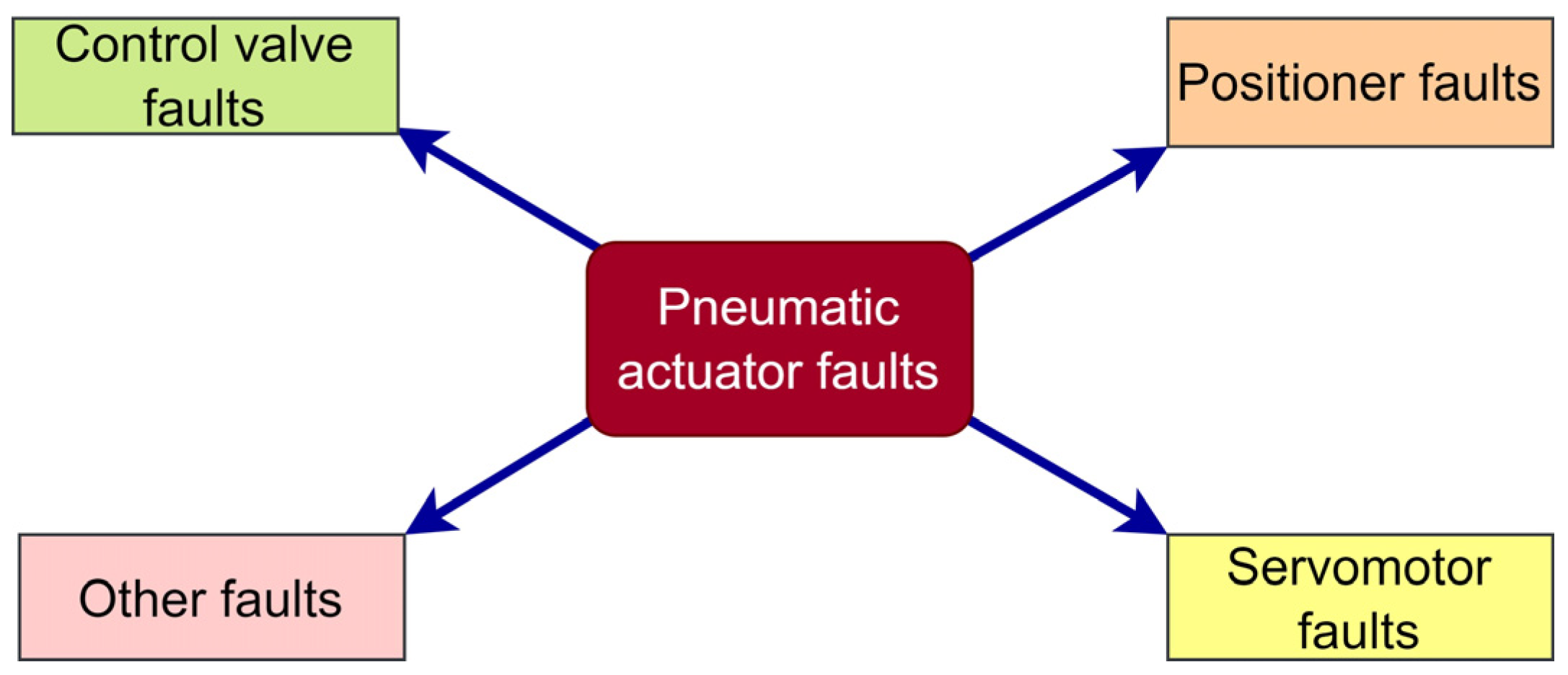
Figure 1. Pneumatic actuator fault categories.
Asi 07 00104 g001
Figure 2. Stiction representation.
Asi 07 00104 g002
Figure 3. A typical neural network with multiple layers.
Asi 07 00104 g003
Figure 4. Block diagram showing the development of a neural network for fault detection. (a) Training phase. (b) Testing phase.
Asi 07 00104 g004
Figure 5. Signal and logic flowchart for the data-driven stiction model.
Asi 07 00104 g005
Figure 6. Open-loop simulation results of the data-driven stiction model.
Asi 07 00104 g006
Figure 7. Closed-loop simulation results of the flow process with the data-driven stiction model.
Asi 07 00104 g007
Figure 8. Closed-loop response of the system without any disturbances. (S = 5, J = 5).
Asi 07 00104 g008
Figure 9. Closed-loop response of the system with Gaussian distributed noise (S = 5, J = 5).
Asi 07 00104 g009
Figure 10. Process variable and controller output of chemical loop 1 (has stiction).
Asi 07 00104 g010
Figure 11. D-value of CHEM loop 1 (has stiction).
Asi 07 00104 g011
Figure 12. PCA of CHEM Loop 1 (has stiction).
Asi 07 00104 g012
Figure 13. Matrix representation of the training data (input and output).
Asi 07 00104 g013
Figure 14. Performance of different learning algorithms for D-values.
Asi 07 00104 g014
Figure 15. Performance of different learning algorithms for PCA.
Asi 07 00104 g015
Table 1. Parameters used to generate artificial data (with stiction).
ParameterDescriptionParameter Range
SStick–slip parameters0.1: 0.25: 10
JStick–jump parameters0.1: 0.25: 10
VWhite noise variance0, 0.010.5, 0.020.5, 0.030.5, 0.040.5, 0.050.5
Table 2. Parameters used to generate artificial data (without stiction).
ParameterDescriptionParameter Range
KpController gain1: 0.05: 2
KIIntegral gain0.05: 0.01: 0.3
VWhite noise variance0, 0.010.5, 0.020.5, 0.030.5, 0.040.5, 0.050.5
Table 3. Parameters used to generate artificial data with external disturbance/oscillation (without stiction).
ParameterDescriptionParameter Range
AAmplitude1: 0.5: 2.
f Frequency0.01: 0.01: 0.11
φ Phase0: 0.25π: 1.75π
VWhite noise variance0, 0.010.5, 0.020.5, 0.030.5, 0.040.5, 0.050.5
Table 4. Performance of each noise level for the D-value.
VariancePerformance %
0.050.569.24
0.040.573.4
0.030.565.9
0.020.565.8
0.010.562.3
Table 5. Performance of various learning algorithms for D-values.
Learning AlgorithmPerformance %
Conjugate Gradient with Powell/Beale Restart (CGB)60.317
Fletcher–Powell Conjugate Gradient (CGF)60.31
Polak–Ribere Conjugate Gradient (CGP)57.53
Scaled Conjugate Gradient (SCG)76.38
One Step Secant (OSS)65.47
Table 6. Performances of various learning algorithms for PCA.
Learning AlgorithmPerformance %
Conjugate Gradient with Powell/Beale Restart (CGB)61.11
Fletcher–Powell Conjugate Gradient (CGF)51.98
Polak–Ribere Conjugate Gradient (CGP)50.19
Scaled Conjugate Gradient (SCG)61.90
One Step Secant (OSS)54.36
Disclaimer/Publisher’s Note: The statements, opinions and data contained in all publications are solely those of the individual author(s) and contributor(s) and not of MDPI and/or the editor(s). MDPI and/or the editor(s) disclaim responsibility for any injury to people or property resulting from any ideas, methods, instructions or products referred to in the content.