Article

Investigating the Influence of Fluid-Structure Interactions on Nonlinear System Identification

by
Skriptyan N. H. Syuhri
*,
Hossein Zare-Behtash
and
Andrea Cammarano
James Watt School of Engineering, University of Glasgow, Glasgow G12 8QQ, UK
*
Author to whom correspondence should be addressed.
Vibration 2020, 3(4), 521-544; https://doi.org/10.3390/vibration3040032
Submission received: 19 September 2020 / Revised: 17 November 2020 / Accepted: 4 December 2020 / Published: 9 December 2020
(This article belongs to the Special Issue Data-Driven Modelling of Nonlinear Dynamic Systems)

Abstract

:
A complex fluid-structure interaction can often create nonlinear dynamic behaviour in the structure. This can be better estimated using nonlinear modal analysis, capable of identifying and quantifying the nonlinearity in the structure. In this study, the case of a vibrating beam submerged in liquid using a nonlinear parameter identification method is presented. This system is considered as an alternative propulsion mechanism, hence understanding the interaction between the fluid and the structure is necessary for its control. Here, impulse signals are used to characterise the numerical and experimental dynamics response of the system. Since the transient responses contain of a multi-component vibratory signals, a vibration decomposition method is used to separate the time response signals based on the dominant amplitude in the frequency response function. The separated time-series signals are then fitted to the nonlinear identification method to construct the backbone and damping curves. The modal parameters obtained from experimental data are then used as a base for the development of the analytical models. The analytical approaches are based on the Euler-Bernoulli beam theory with additional mass and quadratic damping functions to account for the presence of the fluid. Validations are carried out by comparing the dynamic responses of the analytical and experimental measurements demonstrating the accuracy of the model and hence, its suitability for control purposes.

1. Introduction

There are many examples of living organisms (e.g., flagellates, snakes, sandfish) which use body undulations to create propulsion by inducing motion in the fluid surrounding their bodies. Taking inspiration from these examples, alternative propulsion systems that use travelling waves can be devised. Bio-inspired mechanisms based on the application of travelling waves have been considered for novel designs, leading to innovative motors, pumps and transport devices [1]. In particular, this idea played a fundamental role in mechanism-miniaturisation and led to the development of the smallest motor and pump ever conceived [2]. One of the most common configurations to recreate a propulsion system in a fluid environment is by using an elastic beam to generate bending travelling waves. Such innovative devices can be made by simply manipulating the constraints of the beam. For example, in the transport device, an artificial swimmer is created by attaching a permanent magnet at the tip of a free-free beam [3]. By inducing magnetic fields around the beam, travelling waves can propagate through the beam and, by interacting with the surrounding fluid, generate thrust. In micropumps [4,5,6], a fixed-fixed beam is mounted on the top of a micro-channel to generate travelling waves for carrying the fluid inside a micro pipe. A fixed-free beam model can also be used to create a micro-devices for either sensing or pumping purposes [7,8]. Based on these wide range of applications, studies on beams submerged in fluid environments is both challenging and extremely timely.
The interaction between the beam and surrounding fluid in these applications creates a multi-physics problem, often referred to as Fluid-Structure Interaction (FSI). To capture the full behaviour of FSI problems, nonlinear equations that take into account the near field response in proximity of the structure with the large deformations of the structure are necessary. The correct representation of this problem requires a coupling algorithm capable of representing the mutual forces between fluid and solid whilst preserving the continuity conditions in terms of displacements across the fluid-structure interface [9]. Due to the complex nature of these problems, experiments [5,6,10] and numerical modelling [11,12,13] are the preferred approach, leaving little space for analytical models. Consequently, the optimisation of systems designed around FSI principles is complex and expensive, both in terms of computational resources and time. Therefore, minute changes in the structure or fluid parameters would require a substantial computational effort.
To approximate the motion of the beam interacting with a fluid, the complexity in the FSI model is often reduced with assumptions that the presence of the fluid introduces a quadratic damping function and an additional mass in the linear mass per unit length of the beam [14,15,16]. These assumptions have been widely used in numerical simulations investigating the influence of different geometric shapes [8,12], structural and fluid dynamic parameters [8,17]. Similar approaches have been used to detect damage in a structure submerged in fluid [18] and explore the thrust generation in swimming animals [19]. In particular, the quadratic damping function is simplified with linear damping to obtain exact solutions [20,21]. This method, for instance, was used in [21] to present a study on wave transmission aimed at enhancing the travelling wave and cancelling the standing wave formation.
Numerous factors contribute to the generation of damping—e.g., aspect ratio [22,23] and fluid properties [13,24,25]—therefore estimating the exact damping values can be quite challenging. Nonetheless erroneous damping estimations result in considerable errors in the prediction of the dynamic responses, therefore this has been the topic of several research works. The most common technique for calculating the damping is the quadrature peak picking method [26] (or the half-power point method in [27]) which is largely used in FSI characterisations [13,22,23,25,28]. Some low excited modes can create a distorted peak in the frequency response function which leads to an error in the quadrature peak picking method. For this reason, Vu et al. [29] used an advanced modal parameter, based on the time domain method utilising multivariable autoregressive model, to review the damping changes in the modes of the submerged vibrating plate. Alternatively Liu et al. [30] used the PolyMAX algorithm demonstrating that this led to comparable modal damping characteristics. All these methods however can only extract the linear damping; in cases, where the effects of nonlinearities cannot be neglected, a local linearisation of the damping curve is used in the estimation process. Due to the rapid development of the nonlinear identification method, there are currently many tools readily available for extracting modal parameters containing nonlinearities.
In this work, the nonlinearity of a beam immersed in liquid is assessed by a nonlinear parameter identification method developed by Londoño et al. [31]. The method was chosen due to its simple strategy for computing the relation between instantaneous amplitude and frequency. This will give prompt results for identifying nonlinearities from very few decaying peaks in the oscillations. Furthermore, the use of free vibration to investigate nonlinearities is favourable in this study where the responses tend to decay in a swift manner, leading to a reduced computational time compared to that of the forced vibration method. The procedure used in this work is slightly modified: it uses a particularly designed pattern in the train of impulse to maximise the amount of information that can be extracted from a single experiment. Instead of using the Resonance Decay Method [32], step input signals of arbitrary amplitude will be used for generating transient responses so that the structure can experience different force levels. This will allow for the characterisation of the system response over a wider range of amplitudes, resulting in a larger portion of the damping and elastic backbone curves. In fact, the vibration response will contain a multitude of time varying signals with different amplitudes. This can be used to study the mode contribution and the frequency content of the system response. Since each mode may have a distinct decay rate, the time-varying vibration signals is separated in several components based on the largest mode contribution. A detailed description of the technique is provided in the following section.
The aim of this paper is to investigate the nonlinearity of a beam in fluid to improve the approximate models for predicting its dynamics. The novelty in this study is the utilisation of the aforementioned parameter identification technique to evaluate the damping functions. The paper is structured as follows: Section 2 provides an overview of the vibration separation and the nonlinear identification; procedures for generating transient response from experimental and numerical models are presented in Section 3; investigations into frequency content, vibration separation as well as constructing the backbone and damping curves are presented in Section 4; In Section 5, analytical models are developed using the modal parameters estimated from the experiments and numerical results are generated for validation and verification. Finally, conclusions are drawn in Section 6.

2. Theoretical Study

2.1. Vibration Decomposition

The Hilbert Vibration Decomposition (HVD) presented in [33] is one of the methods for extracting non-stationery as well as multicomponent vibratory signals. This technique is primarily based on the assumption that the signal can be represented as a sum of time-varying components with different amplitudes and frequencies [34]. Therefore, it is not applicable for separating a signal composed of a superposition of the same amplitude and frequency.
There are four major steps required to decompose a signal: estimating the dominant frequency, applying a low-pass filter, calculating the amplitude as well as the phase shift correction, and finally, subtracting the decomposed from the initial signal. Figure 1 illustrates the HVD procedure used for vibration decomposition. The analytic signal is used to examine the direct vibration properties, such as instantaneous vibration amplitude, frequency and phase utilising the Hilbert Transform. The key for smooth decomposition results is the use of a low-pass filter after the derivative of the instantaneous phase angle. The filter removes the high frequency components which create small oscillations in the time series of the instantaneous frequency.
The purpose of the synchronous demodulation is to calculate the respective amplitude from the estimated frequency. A signal with the estimated frequency and amplitude of the forcing signal is multiplied with the measured signal. This operation is repeated twice: in the first case the reconstructed forcing signal is used, in the second case the same signal is shifted of 90° as follows [35],
x ( t )   =   0.5 A ( t ) cos φ ( t )
x ˜ ( t ) = 0.5 A ( t ) sin φ ( t )
where x ( t ) is the initial signal from measurement and has a real value, A ( t ) is the instantaneous amplitude, φ ( t ) is the instantaneous phase and t is the time. The result will be a signal proportional to the in-phase (Q) and out-of-phase (I) components of the input. Low-pass filters are used to remove high-frequency errors. The magnitude of the input signal is calculated by taking the sum of the squares of I and Q, whereas the phase is evaluated by taking the arctangent of the ratio Q/I.
The amplitude, A i ( t ) , and phase shift, ( t ) , after the demodulation process can be estimated from Equations (1) and (2) using the same techniques as shown in Figure 1. The phase shift correction is important to make the decomposed signal in-phase with the initial or the reference signal. Therefore, only the out of phase signal remains after the subtraction process. The procedure is repeated for an arbitrary number of iterations.

2.2. Nonlinear Identification

There are many procedures for estimating the backbone and damping curves from free vibration. The backbone curve shows the change of instantaneous frequency with respect to the instantaneous amplitude. A simple method for assessing the instantaneous frequency, f ( t f i ) , is presented by Londoño [31] which considers the inverse of the instantaneous period as follows,
f ( t f i )   =   1 ( t f i + 1 t f i 1 )
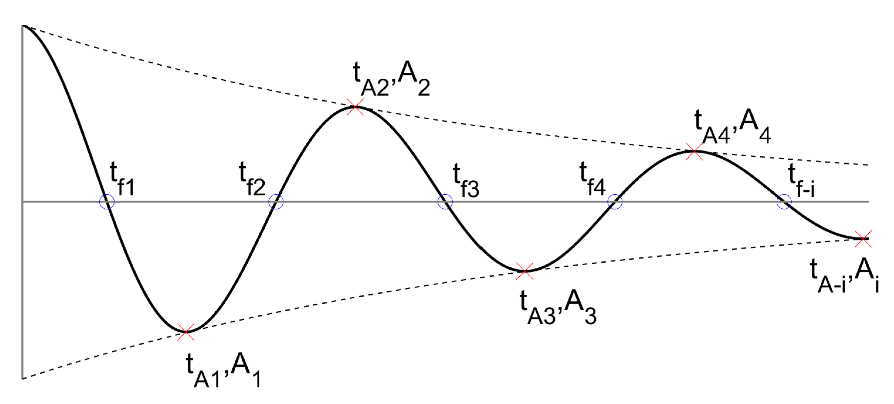
where t f i is the series of the zero crossing time, i   =   [ 1 ,   2 ,   3 , ] , as illustrated with the blue circle markers in Figure 2. Theoretically, the crossing time is determined at the amplitude equal to zero, A   =   0 . However, t f i is often acquired from a decay response at amplitude close to zero, A 0 , due to discretisation of the signal. This condition leads to a noisy instantaneous frequency which requires a filter to smooth out the result or an interpolation algorithm to obtain an ideal t f i at A   =   0 .
The instantaneous amplitude can be observed by tracing the local minima or maxima from each zero-crossing point of the transient response as indicated by the red cross markers in Figure 2. Since the frequency is calculated based on one cycle of the curve, the number of the instantaneous frequency data would be equal to that of the instantaneous amplitude, [ f ( t f i ) ] m × n   =   [ A ( t A i ) ] m × n . Therefore, the backbone curve can be compiled by pairing these data.
The damping curve can be estimated by assuming that the decaying envelope, A ( t ) , has a function of the form,
A ( t )   =   A 0 e ζ ( t ) 2 π f ( t ) t
where A 0 is the initial amplitude, ζ ( t ) is the damping ratio and f is the instantaneous frequency. The damping ratio coefficient can be determined by using linear regression analysis of Equation (4) as follows,
{ ln | A ( t 0 ) | ln | A ( t 1 ) | ln | A ( t N 1 ) | }   =   [ 2 π f ( t 0 ) t 0 1 2 π f ( t 1 ) t 1 1 2 π f ( t N 1 ) t N 1 1 ] { ζ ( t ) ln | A 0 | }
where N is the number of data points. In other words, the linear damping ratio is extracted from the gradient of a straight line when it is plotted in a logarithmic scale with respect to time. The damping, however, can be represented with quadratic or even cubic functions. The coefficients for those functions can be found using linear regression analysis. The nonlinear damping in Equation (4) may be written as
A ( t )   =   A 0 e ( k 1 t 3 + k 2 t 2 + k 3 t )
where the coefficients k 1 , k 2 , and k 3 can be evaluated, according to [36], using the least-square solution to
{ ln | A ( t 0 ) | ln | A ( t 0 ) | ln | A ( t N 1 ) | }   =   [ t 0 3 t 0 2 t 0 1 t 1 3 t 1 2 t 1 1 t N 1 3 t N 1 2 t N 1 1 ] { k 1 k 2 k 3 ln | A 0 | }
Note that, although the coefficients of the nonlinear expansion of the damping are sought, the method used in Equation (7) is linear in its nature.

3. Materials and Methods

The system under consideration is illustrated in Figure 3, where x and z define the physical coordinate system. The beam is coupled with a permanent magnet at one side and free at the other end. The magnet is used to either attract or repel the magnetic fields induced by an electromagnet situated around the structure, inducing a periodic oscillation in the transverse direction. The beam is composed of a uniform steel alloy material which has a density and modulus of elasticity of 7200 kg/m3 and 240 GPa, respectively. The beam has a rectangular geometry, 80 × 12.75 mm, with a thickness of 0.08 mm. The analysis is carried out in two different fluid media, namely air and water. Thus, the terms “dry” and “wet” will be used here to represent the beam in air and liquid environments, respectively. The air and water density are 1.26 kg/m3 and 997 kg/m3, respectively.

3.1. Experimental Setup

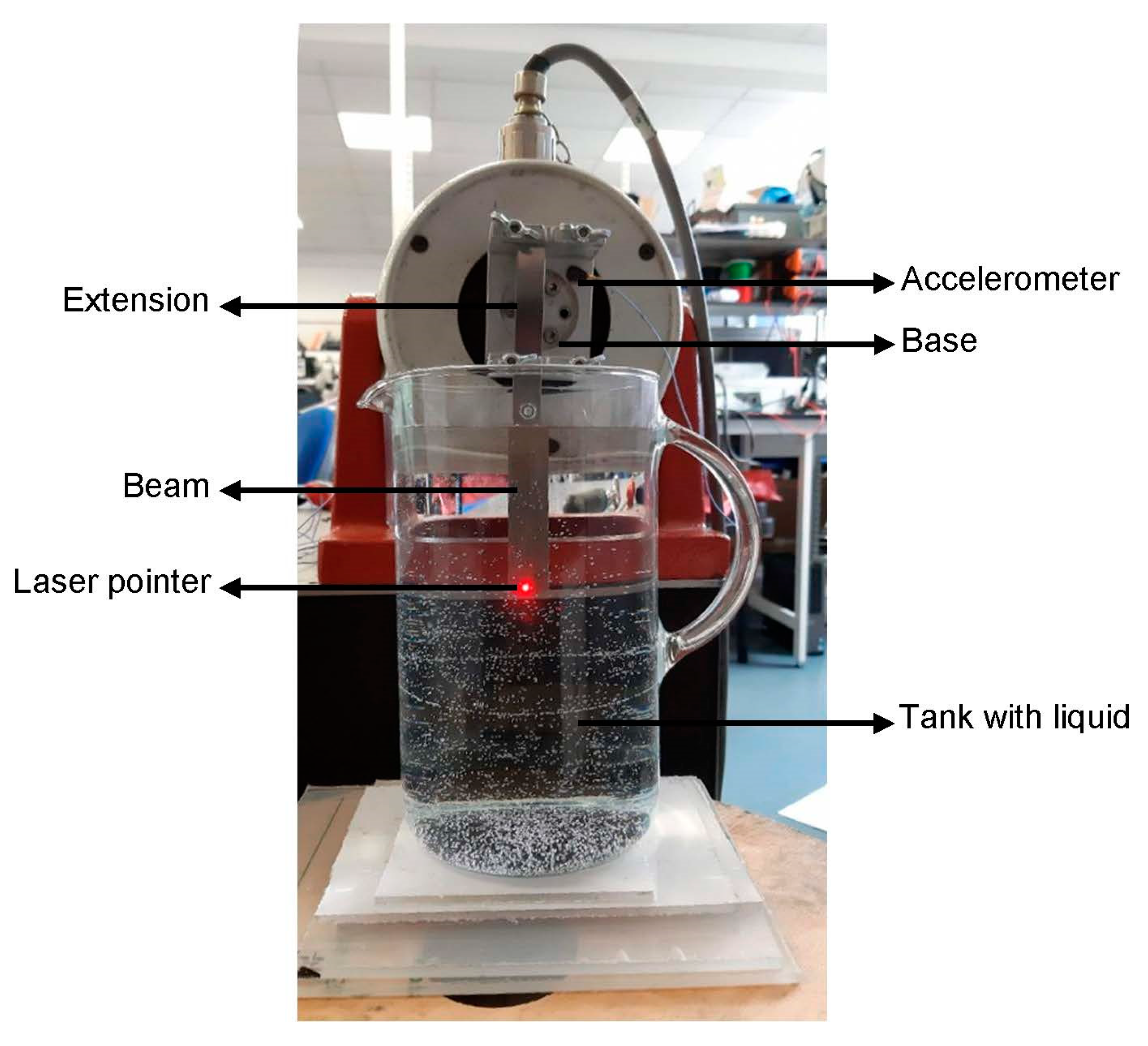
To create an equivalent model of Figure 3, the beam, shown in Figure 4, is clamped on an LDS V406 permanent magnet shaker to induce vibrations in the structure. A rigid extension is used to fully immerse the beam in water and reproduce the rigid body movement of the magnet illustrated in Figure 3. The velocity response of the beam is acquired from a single-pointer Polytech laser vibrometer PDV-100, while the base acceleration, w ¨ b , is measured by an accelerometer. For the purpose of this experiment, the extension can be considered rigid, i.e., its lowest natural frequency occurs far from the frequency range of interest. Figure 4 shows the experimental setup for the beam in the wet condition, whereas, in the dry condition, the tank is simply removed.

3.2. Numerical Simulation

A numerical model capable of simulating FSI is performed using Simcenter STAR-CCM+ to reproduce the behaviour of this multiphysics system. The multiphysics solution is obtained by the simultaneous computation of the solid and fluid domains. These two domains interface through a coupling algorithm such that the fluid and solid exchange forces and displacements across the fluid-structure interface. In the fluid solver, the implicit unsteady approach is used to perform the transient and steady state simulations. The model assumes that the fluid density is steady throughout the continuum. The laminar flow solver is used because the Reynold number is low enough to prevent transition to turbulence. The flow equations such as the momentum and continuity equations are solved in a segregated or uncoupled manner. In addition, the transport equations which describe the mechanics of solid and fluid continua are derived based on gradient computation models.
In the solid domain, the system is modelled using three-dimensional elements and the motion of the beam is restricted to the XZ-Plane to avoid torsion. The material is assumed to be isotropic linear elastic in which only density, Poisson’s ratio and Young’s Modulus are used to define the material properties. Although the model has linear geometry and material, the influence of fluid forces may change the load orientation which results in generating large displacements and nonlinear interactions. Thus, the feature of nonlinear geometry analysis in the solid solver is activated to capture such phenomena. For the boundary conditions, the beam is only allowed to displace in z-direction at x = 0, and free at the other side to emulate the cantilever beam subject to base motion. The displacement is computed via finite element method (FEM). The input for the simulation is in the form of a constant base displacement, w b ( x , t ) , and is assigned as a boundary condition.

4. Nonlinear System Identification

In the following section, the transient responses from experimental and numerical data are presented and analysed by looking at the mode contributions. The first-two dominant modes are then extracted from the decay response using the wave decomposition technique and are used to estimate the backbone and damping curves.

4.1. Dry Model Analysis

To perform a numerical simulation for the dry model, the damping feature in the simulation requires an initial assumption for the coefficients of the mass and stiffness matrices in the Rayleigh damping model. Since the Rayleigh damping can be represented by a modal viscous damping assigned in each mode of the system [37], the mass and stiffness damping coefficients are calculated with an assumption of the damping ratio of 0.2% and 0.1% for the first and second modes, respectively using the proportionality principle. This estimation is based on the common damping assumption for steel which varies between 0.1–0.2% [38].
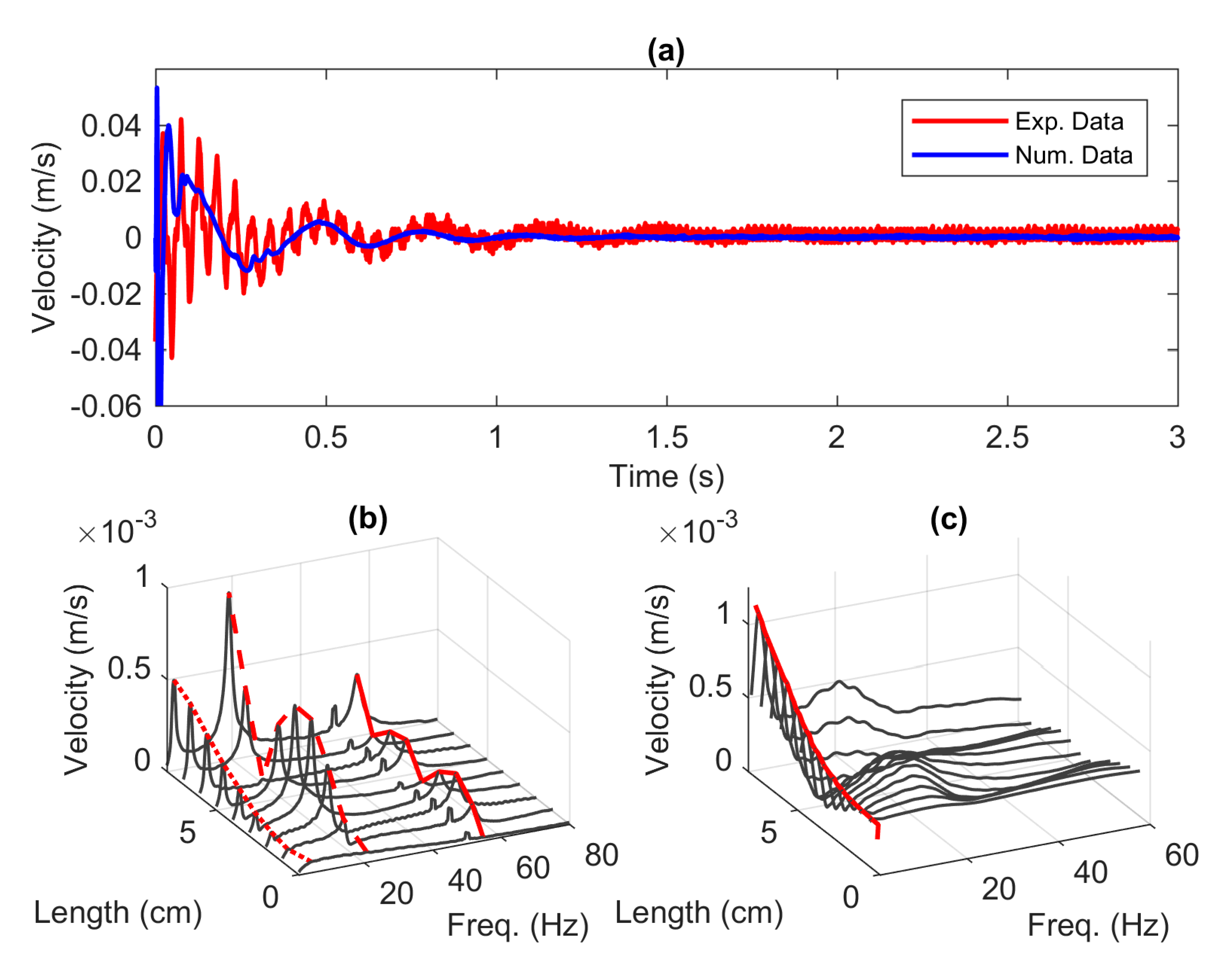
Using the step function as input signal, Figure 5a presents the time series of velocity for both approaches in the dry condition acquired at the tip of the beam, x = L . From the figure, the decay rate appears similar after 5 s for both cases indicating a slow-varying amplitude over time. Nonetheless, at the beginning of the free decay measurement a rapid decay in oscillations is observed. This phenomenon is further examined by looking at the frequency domain.
By implementing the Fast Fourier transform (FFT), the frequency responses are depicted in Figure 5b,c for various locations along the length of the beam. From the figures, the red lines over the local maxima (peaks) represent the first, second and third mode shapes of the beam. Note that the peaks appeared at 150 Hz as well as 200 Hz in the experiment data shown in Figure 5b are the aliasing errors. It can be seen from Figure 5b,c that the two models have different mode contributions. The numerical model has equal first and second mode contributions, while the first mode contributes the most in the experiment model. This occurrence can be related to the structure of the clamped section of the beam depicted in Figure 4. The beam is mounted on the moving part of the shaker where this element is held up by a flexible support that acts like a spring [27]. Therefore, there is a possibility that the moving part of the shaker absorbs vibrations. We also noticed from physical observations that, before the base of the shaker reaches the steady state, it goes through an overshoot followed by a small oscillation in response to the step input signal. This phenomenon, however, will be investigated in detail in the next section.
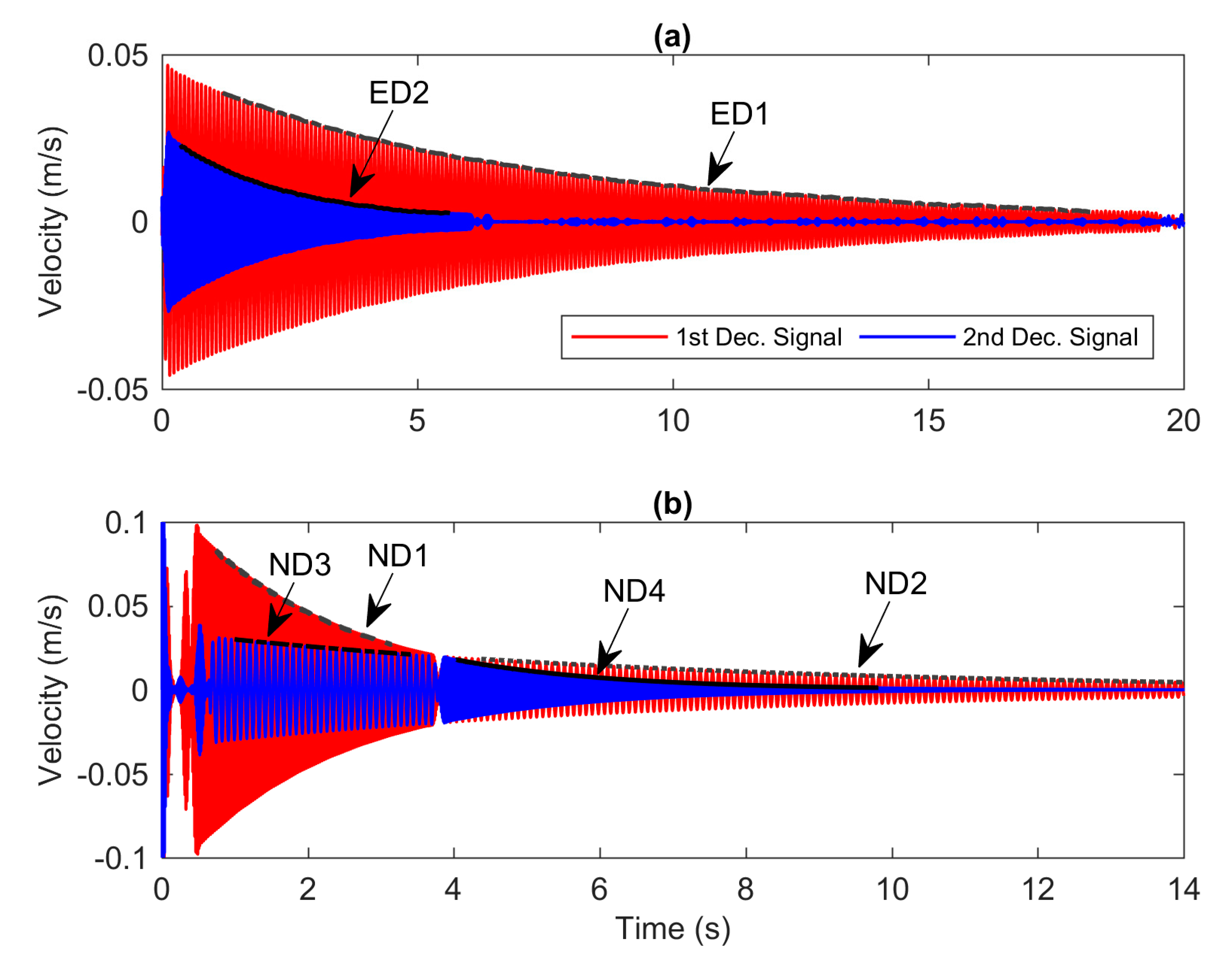
To examine the nonlinearity in each mode, the time series of velocity shown in Figure 5a is decomposed using the wave separation technique presented in Section 2.1 to extract the first and second modes. The third mode is not taken into account since it has very little contribution in the experimental model. Therefore, there are only two iterations in the block diagram of the HVD procedure as illustrated in Figure 1. Figure 6a,b present the decomposed signals for the experimental and numerical models, respectively. The red and blue colours from both figures signify the first and second decomposed signals, respectively. The notations ED1, ED2, ND1, ND2, ND3 and ND4 represent the instantaneous amplitudes of the experimental (ED) and numerical data (ND). It is seen from the figures that the amplitude of the decay response can be associated with the mode contributions in the frequency domain of the initial signal. For instance, the initial amplitudes of the first and second decomposed signals of the experimental model shown in Figure 6a have the same proportion as the peaks of the initial signal in the frequency domain. In Figure 6b, interestingly, there are two distinct decay rates and frequencies in one signal. We can assume that ND2 and ND3 have similar instantaneous frequency properties and demonstrate very slow decaying rate compared to that of ND1 and ND4. The distinction in the decay rate is of course due to the assumption that the damping ratio for the first mode is set to a higher value than for the second mode.
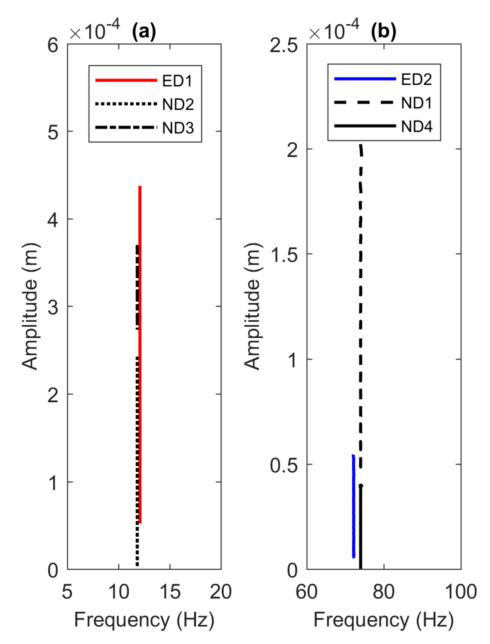
The time series of velocity shown in Figure 6 is integrated numerically to obtain the relative displacement of the beam. Using the nonlinear identification method to extract the instantaneous amplitude and frequency presented above, the backbone curves for the first and second mode are depicted in Figure 7a,b. From the figures, the backbone curves indicated with the legends ED1—ND4 are extracted from the instantaneous amplitudes shown in Figure 6. The instantaneous frequencies however are not shown here for brevity. The backbone diagrams exhibit a straight-line indicating that the system behaves linearly. The difference between the estimated frequency values between the experimental and numerical models can be related to the filtering process in the HVD procedure to smooth out the analytical signal, the instantaneous vibration properties and the demodulation process. Nevertheless, the disparity between the two models are insignificant with errors less than 3% for the two modes.
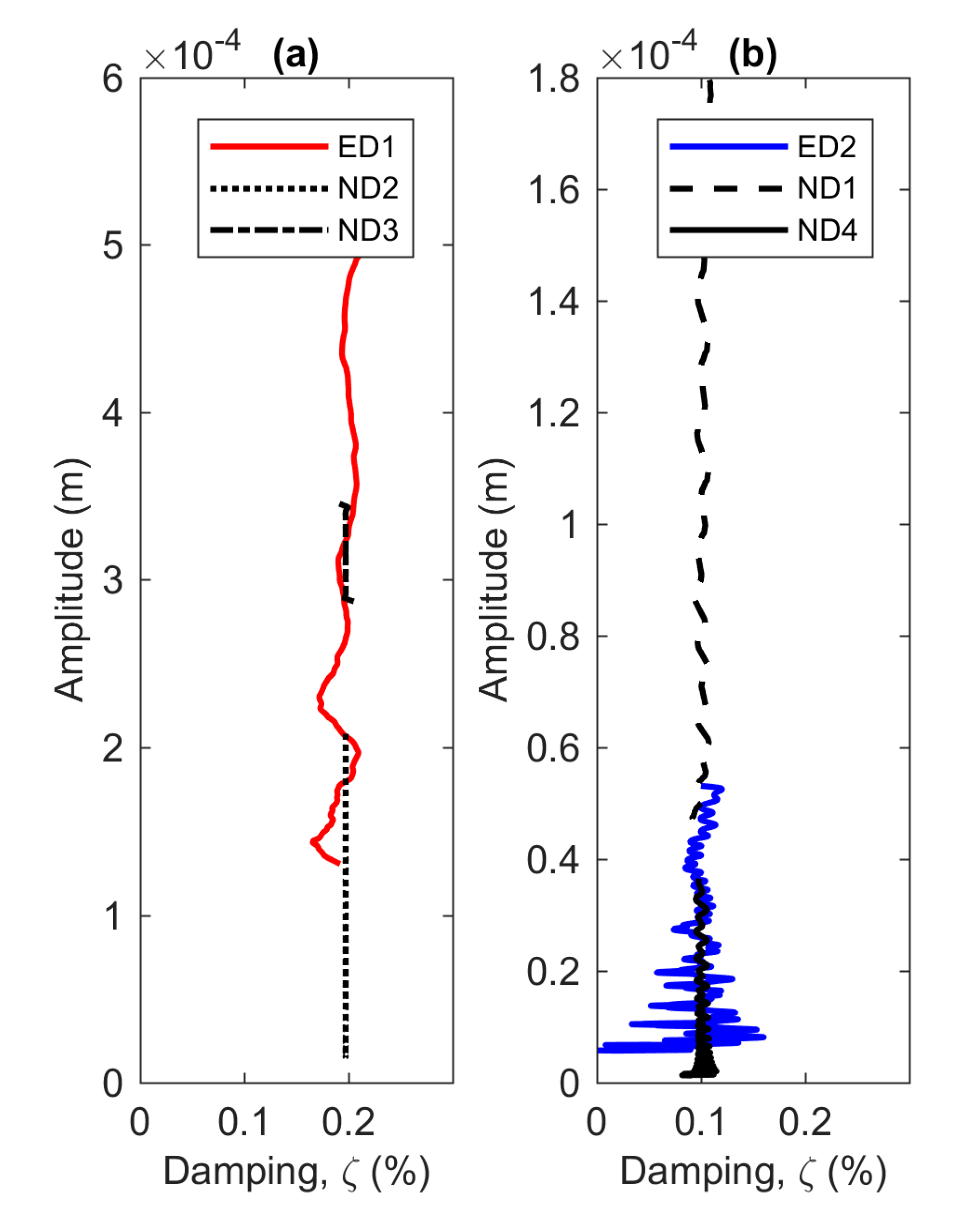
Figure 8a,b display the damping curve with respect to the displacement amplitude. As expected, the experimental and numerical models exhibit linear damping characteristics. The damping curves of the experimental and numerical results coincide with each other and agree with the initial assumption of 0.2% and 0.1% damping ratio for the first and second modes, respectively. The presence of noise in the second mode of the experimental model is due to rapid decay time of this mode. It is worth noting that the purpose of the dry model analysis is not only for characterising the beam in air, but also to prove that the procedures for identifying the nonlinear system are correct.

4.2. Wet Model Analysis

The first test for the wet model was carried out using the step function input signal. Figure 9a shows the time series of the velocity response obtained at the tip of the beam. The results show a satisfactory performance of the numerical model in order to replicate the response of the experimental model, albeit with less oscillation. The frequency responses reveal that the three modes of the experimental model appear just under 60 Hz as shown in Figure 9b. On the other hand, the only obvious peak in the numerical model shown in Figure 9c is the first mode marked with the continuous red line over the peaks along the beam length. The second and third modes exhibit highly damped characteristics indicated with a rounded peak. There is no clear peak particularly in the third mode which are hard to detect using standard algorithm to extract the local maxima. However, it can be seen from visual observation that the patterns around 20 Hz and 60 Hz form the mode shapes of the second and third resonant frequencies.
Figure 10a,b depict the decomposed signals of the experimental and numerical models, respectively. From both figures, only the first decomposition signals indicated with the red lines provide very apparent decaying oscillations. The envelopes over the decay signals denoted with “EW1” and “NW1” signify the instantaneous amplitude of the experiment and numerical models respectively. The envelope is chosen such that it is favourable for nonlinear identification analysis. It is reasonable to assume that EW1 corresponds to the contribution of the second mode of the experimental model, while NW1 is under the influence of the first mode of the numerical model. The identification process for the numerical model becomes challenging since the envelope of NW1 contains a short time period signal where the amplitude tends to decay very quickly. Consequently, the instantaneous amplitude is comprised of a very few data points from several peaks for nonlinear analysis.
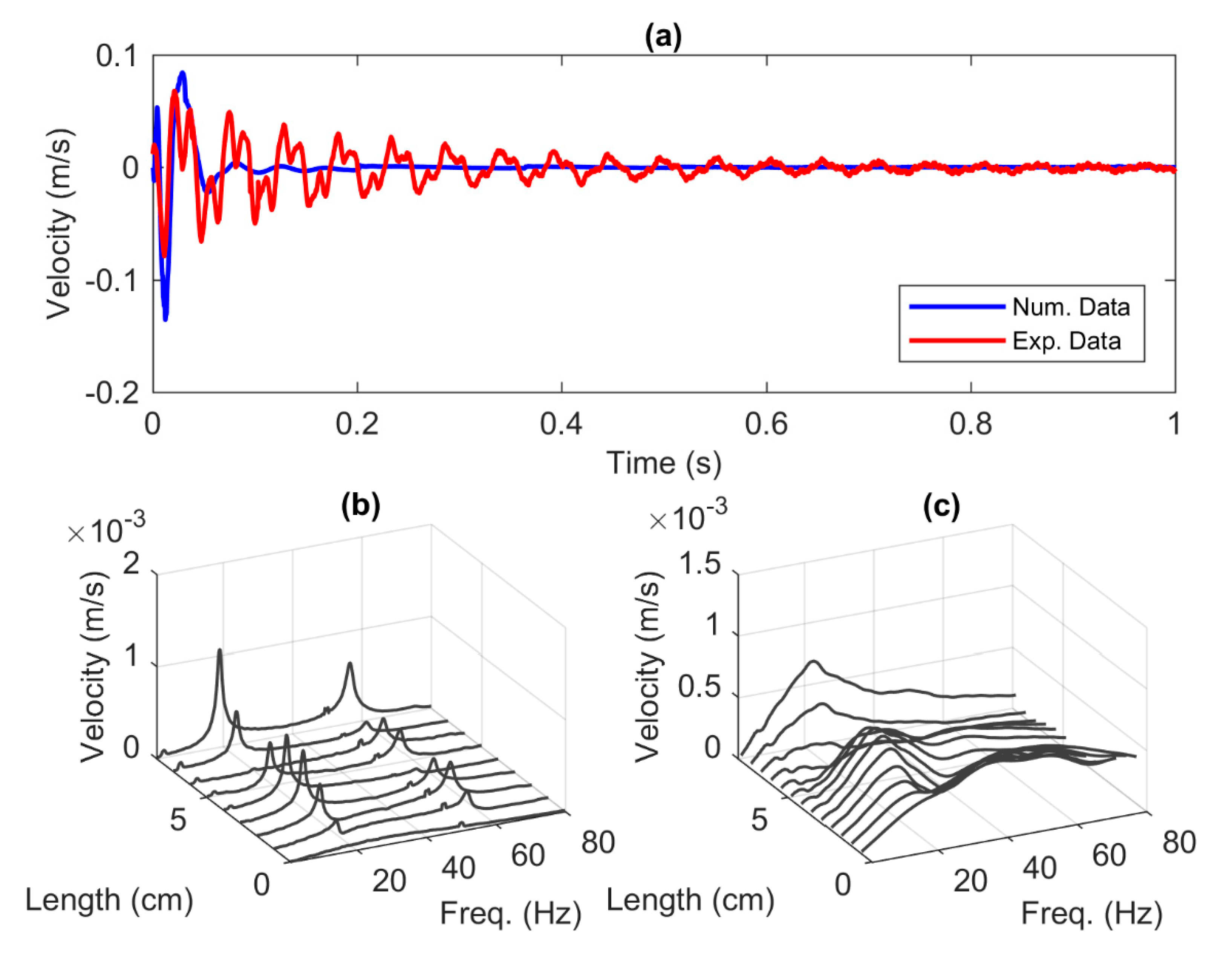
The second test was carried out with the derivative of ramp function. Figure 11a shows the comparison of the time series of the experimental and numerical models acquired at the tip of the beam. Although the first trough and peak have almost the same period and magnitude, it can be seen from the figure that the oscillation of the numerical model decays faster than before. In contrast, the waveform of the experimental model tends to oscillate longer and contains multiple frequencies. To investigate this, the frequency response of the numerical model is plotted in Figure 11b. As expected, the input signal successfully excites the second and third modes with the least contribution of the first mode. The same phenomenon is also demonstrated by the numerical model shown in Figure 11c where the dominant peaks lie within the range of the second mode. Although the high damping properties hides the presence of the third mode.
The decomposed signals from the decay responses are plotted in Figure 12. In the experiment model shown in Figure 12a, the second and third modes are successfully extracted from the initial signal where the decaying oscillations provide a promising instantaneous amplitude for nonlinear modal analysis indicated with the envelope EW2 and EW3. However, the decomposition of the numerical model shown in Figure 12b suggests a very short period of the signal. The envelope of NW2 shows very few peaks that can be acquired from the signal. Therefore, the NW2 is not sufficient to be used in the system identification procedure.
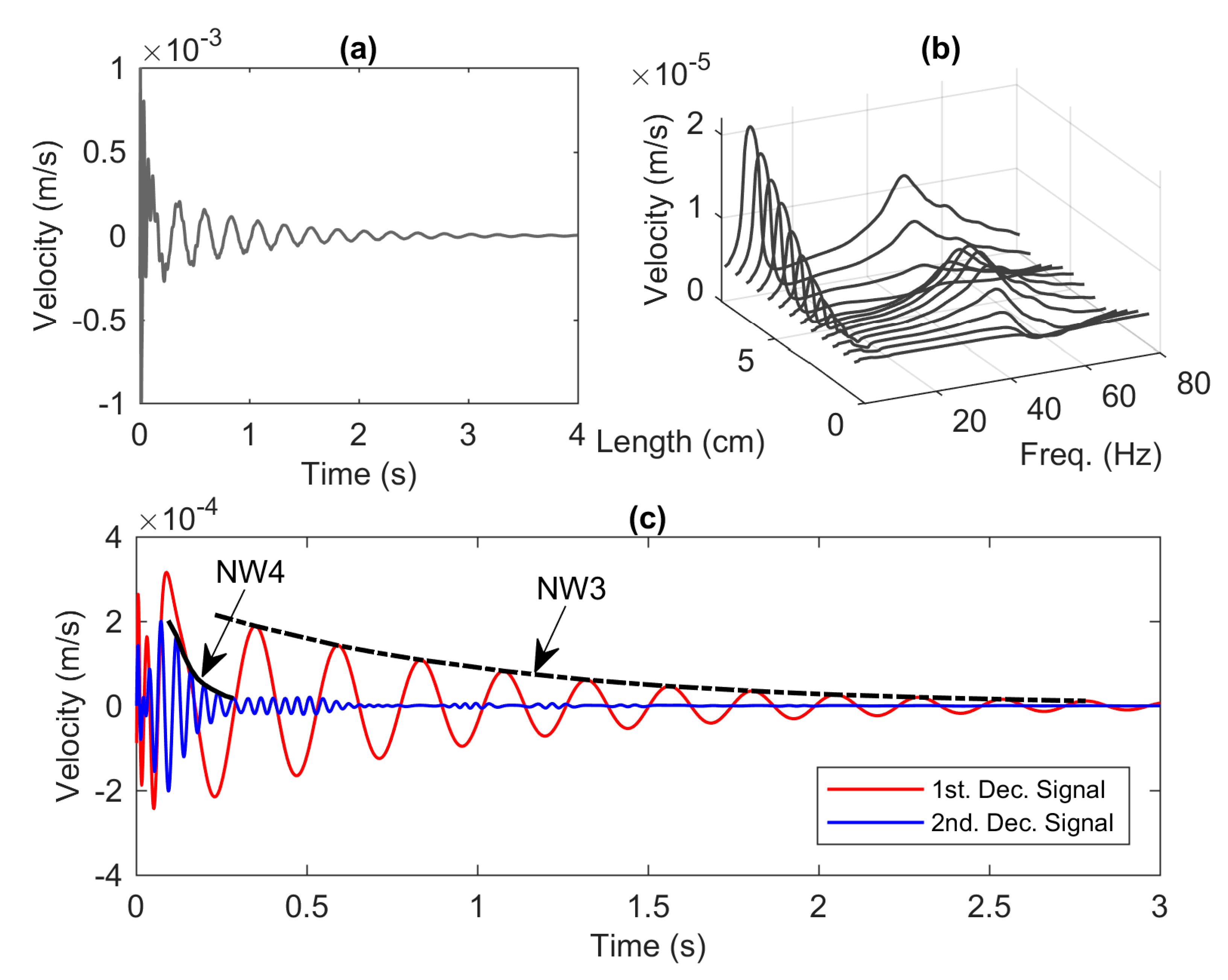
For this purpose, we use the numerical model to produce a decaying signal to fit with the number of data points of the nonlinear identification system. There are some techniques to increase the oscillation such as increasing the inner iteration of the fluid solution or loosening the fluid mesh size. These techniques would reduce the coupling of the fluid and structure leading to a decrease in the fluid damping on the beam. However, it is worth mentioning that these methods create a noticeable error in the natural frequency due to lack of the added mass. Consequently, the validation with the experimental data is no longer valid. Alternatively, the amplitude of the input signal is reduced to lessen the influence of the fluid damping without affecting the added mass. The terms of fluid damping and added mass will be discussed in the next section in detail.
Figure 13a shows the time series of velocity generated using the step input with the base amplitude of 0.01 mm. It is seen that the response undeniably oscillates for 4 s. The frequency response shown in Figure 13b unveils that the second mode becomes prominent compared to that of the frequency response in Figure 9c. Interestingly, the value of the second mode moves away from the origin and becomes less important compared to that of the experiment model. Figure 13c exhibits the two separated signals using the signal separation presented in Section 2. The first decomposed signal, indicated with the red line, has a pronounced envelope, NW3, with slow-varying amplitude over the period of time.
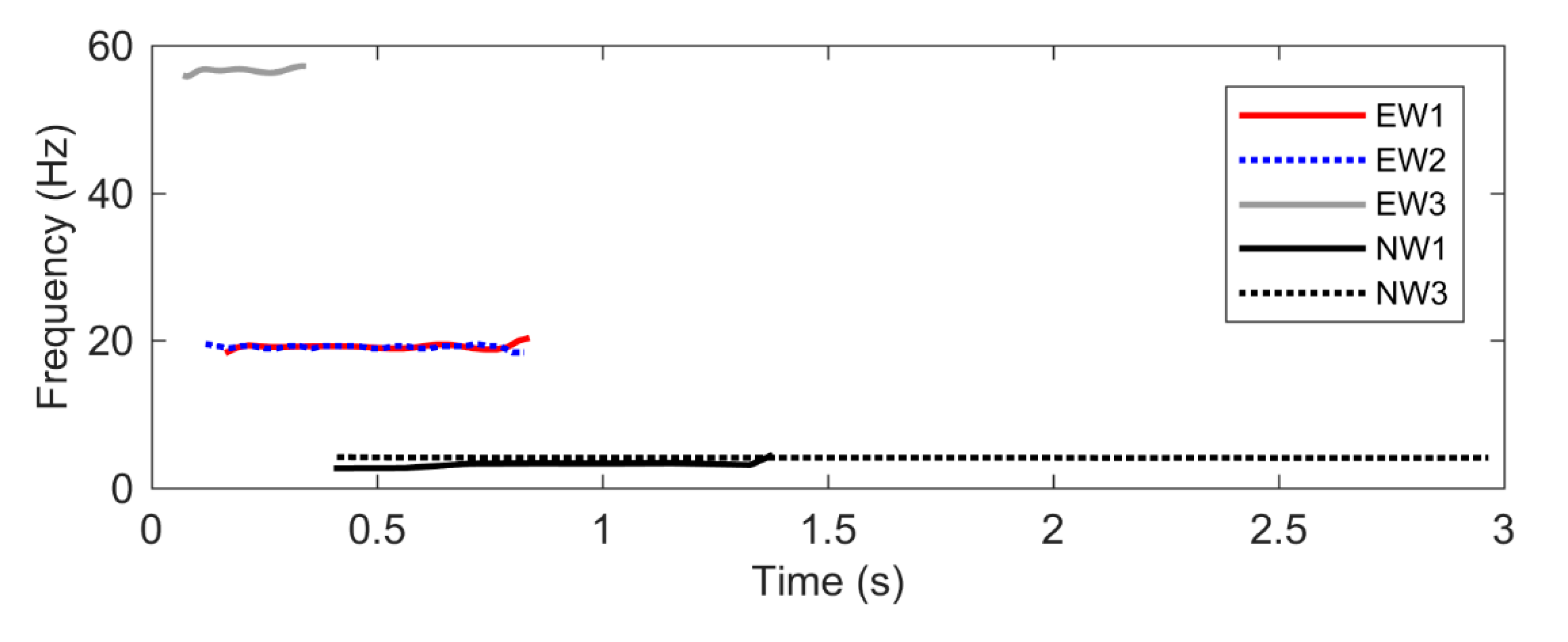
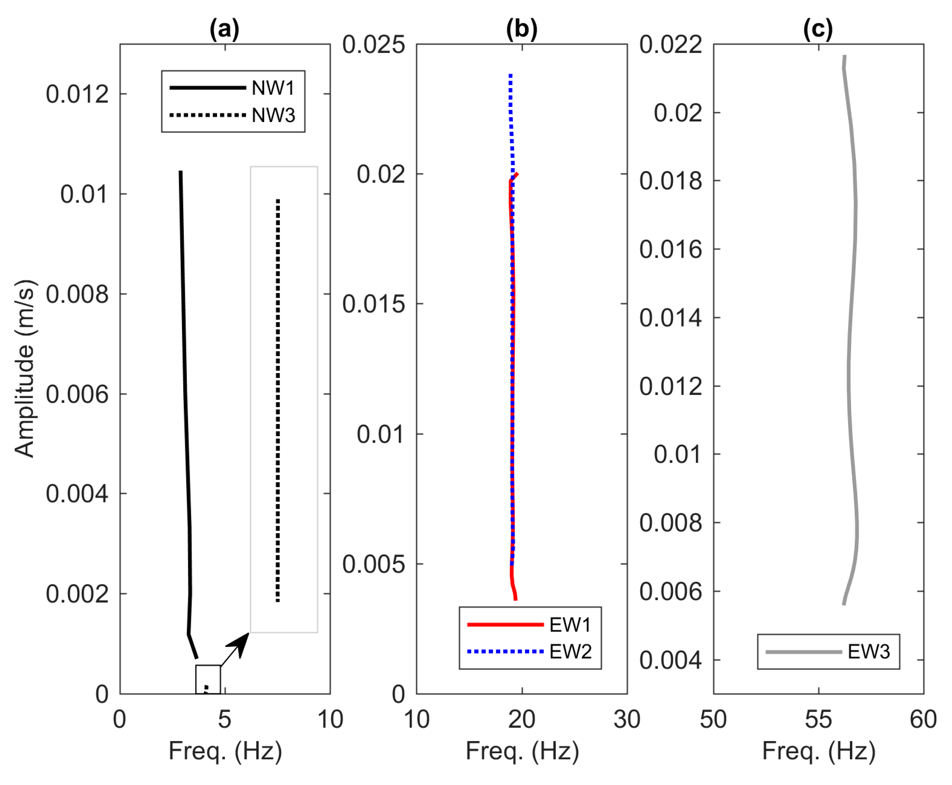
Figure 14 depicts the time series of the instantaneous frequency extracted from the decay responses of the envelopes EW1, EW2, EW3, NW1 and NW3. From the figures, all models agree that there is no sign of nonlinearity as demonstrated by the unchanging frequency over time. The backbone curves are constructed by pairing those instantaneous frequencies with the instantaneous amplitudes as illustrated in Figure 15. Note that the line NW1 shown in Figure 15a is formed with fewer data points which create bias in the straight line. In addition, the line EW3 shown in Figure 15c is also extracted from the noisy signal of the third mode. Consequently, an arbitrary 5 point moving average filter is applied to smooth out the line where the mean is calculated based on the current point, 5 elements backward and 5 elements forward.
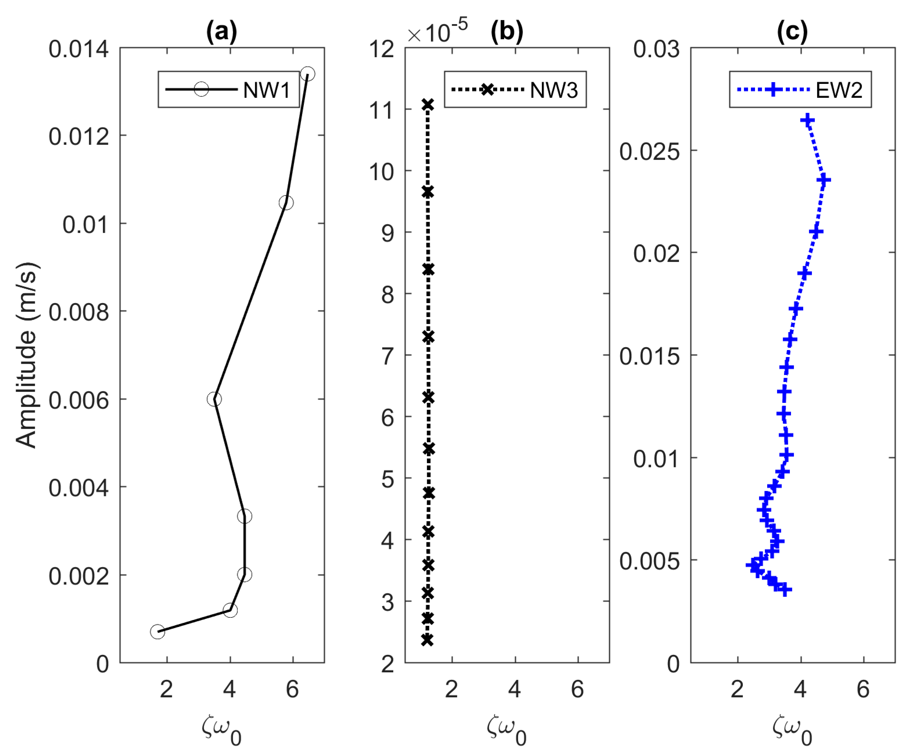
Figure 16 presents the velocity effect on the damping values. The markers on the lines represent the number of data points. Figure 16a shows the damping curve extracted from the envelope NW1. It can be seen that the decay value is in the range of 2 s 1 to 7 s 1 , rapidly reaching steady state in the decay response. Nonetheless, the results are not so sufficient to justify whether the damping is linear or not due to lack of data points. Figure 16b displays the damping curve from the envelope NW3, while the damping curves from the experiments are plotted in the same figure, namely Figure 16c. Interestingly, the results shown in Figure 16a,c have common characteristics where the nonlinearity occurred in high amplitudes. The nonlinearity becomes negligible in the low amplitude as shown in Figure 16b. In addition, the damping curves in Figure 16c will be used as the reference for deriving analytical models capable of predicting dynamics behaviour of the beam.

5. Analytical Approximation Methods

5.1. Analytical Model

From Figure 3, since the magnet has a modulus of elasticity and a material thickness of approximately 100 times greater than those of the beam, the magnet is assumed to undergo rigid body movement in z direction. Thus, the beam can be modelled as a clamped-free beam subject to translation of its base. The beam experiences a relative movement with respect to the base. The absolute (global) displacement, w ( x , t ) , of each point of the beam can be written as [39],
w ( x , t )   =   w b ( x , t ) + w r e l ( x , t )
where w r e l ( x , t ) is the local displacement relative to the clamped end of the beam and w b ( x , t ) is the base movement.
Note that the small rotation effect is neglected for the base motion due to the head constraint. The basic modelling assumption for the beam is that the beam displacement at any point x and time t in the z direction is small compared with the total length, L , of the beam resulting in no axial ( x direction) displacement. Additionally, the thin-beam assumption is used in the analysis, vanishing the shear deformation and the rotary inertia effects. Thus, the linear damped Euler-Bernoulli equation for free beam vibration in the transverse direction can be written as [40],
μ 2 w r e l ( x , t ) t 2   +   C i w r e l ( x , t ) t   +   E I 4 w r e l ( x , t ) x 4   =   0
where C i is the internal damping coefficient caused by the material.
When the beam submerged in fluid vibrates, the fluid around the beam is forced to move. The movement of the fluid generates fluid forces that work on the beam. Those fluid forces depend on the acceleration and velocity of the beam. When the beam is accelerated, the fluid around the beam is forced to accelerate in the same direction. Consequently, it creates a reaction force that is associated with the acceleration. For the rectangular plate, this association, which is called the added mass, M , can be estimated as follows [21]:
M   =   ρ π ( H 2 ) 2
where ρ is the fluid density and H is the beam width.
Similarly, the reaction force that corresponds to the fluid velocity introduces an added damping, f D , on the beam which originates from the fluid viscosity. In the case of no external flow, the damping force, f D , on the beam resulting from fluid motion is written as [15]:
f D   =   C f | x ˙ | x ˙
where C f is the damping coefficient and x ˙ is the local velocity of the beam which is in this case w r e l ( x , t ) / t . Substituting these additional forces into Equation (9), the equation of motion in absolute frame of reference can now be written as, recalling Equation (8),
( μ + M ) 2 w r e l ( x , t ) t 2 + ( C i + C f | w r e l ( x , t ) t | ) w r e l ( x , t ) t + E I 4 w r e l ( x , t ) x 4   =   ( μ + M ) 2 w b ( x , t ) t 2
Note that unlike the previous equations, Equation (12) becomes the damped Euler-Bernoulli equation with a time-varying distributed load.
The solution of the damped Euler-Bernoulli equation can be represented by an infinite series of separation variables involving space and time functions,
w r e l ( x , t )   =   i = 1 W n ( x ) q n ( t )
where q n ( t ) represent the generalized modal coordinate or the modal displacement of the beam in the n -th mode and W n ( x ) is the normal mode-shape in the n -th mode corresponding to undamped free vibration. The corresponding mode shape can be determined from the boundary conditions in which the clamped-free boundary conditions give [26],
w r e l ( 0 , t )   =   0 ,                   w r e l ( 0 , t )   =   0 ,                   E I w r e l ( L , t )   =   0 ,                   E I w r e l ( L , t )   =   0
Resulting in the normal mode shape, W n ( x ) , of the form
W n ( x ) = cosh β n x L cos β n x L σ n ( sinh β n x L sin β n x L )
where the term refers to the differentiation with respect to the x , β n is the weighted frequencies obtained from the characteristic equation, cos β cosh β   = 1 , and σ n is expressed as
σ n   =   sinh β n sin β n cosh β n cos β n
It is common practice to omit damping terms in the modal decomposition procedure [41]. The damping is introduced to each mode after the decomposition has been applied. This method is somehow mathematically convenient and extremely useful in modelling techniques without loss of generality. Thus, the modal coordinate can be determined by substituting Equation (13) to Equation (12), multiplying the result by an arbitrary mode shape, W m ( x ) , and integrating from 0 to L based on the orthogonality condition to give
( μ + M ) n = 1 0 L W n ( x ) W m ( x ) q ¨ n ( t ) + E I 0 L W n ( x ) W m ( x ) q n ( t )   =   ( μ + M ) 2 w b ( x , t ) t 2 0 L W m ( x )
By using orthogonality conditions, Equation (17) can be expressed as an infinite mode number of independent equations. For the cantilever beam, in the case of m = n , the multiplication of mode shape and its integration over the length of the beam results in [41]:
0 L W n ( x ) W n ( x )   =   L
0 L W n ( x ) W n ( x )   =   β n 4 L 3
Equation (17) may now be simplified using the integrals of Equations (18) and (19), dividing by L , and adding the damping terms to give
( μ + M ) q ¨ n ( t ) + ( C i + C f | q ˙ n ( t ) | ) q ˙ n ( t ) + E I β n 4 L 4 q n ( t )   =   1 b Q n ( t )
where Q n ( t ) are the generalized force given by
Q n ( t )   =   ( μ + M ) 2 w b ( x , t ) t 2 0 L W n ( x ) d x
And the constant b is the normalization condition of the eigenfunctions given by
b   =   0 L W n 2 ( x ) d x
Equation (20) is basically the modal equation for a single mass with multi-degrees of freedom. Since the equation contains a quadratic damping term, the modal displacement, q n ( t ) , can be solved by using, for instance, numerical integration based on Runge-Kutta methods [31].

5.2. Validation of Natural Frequencies

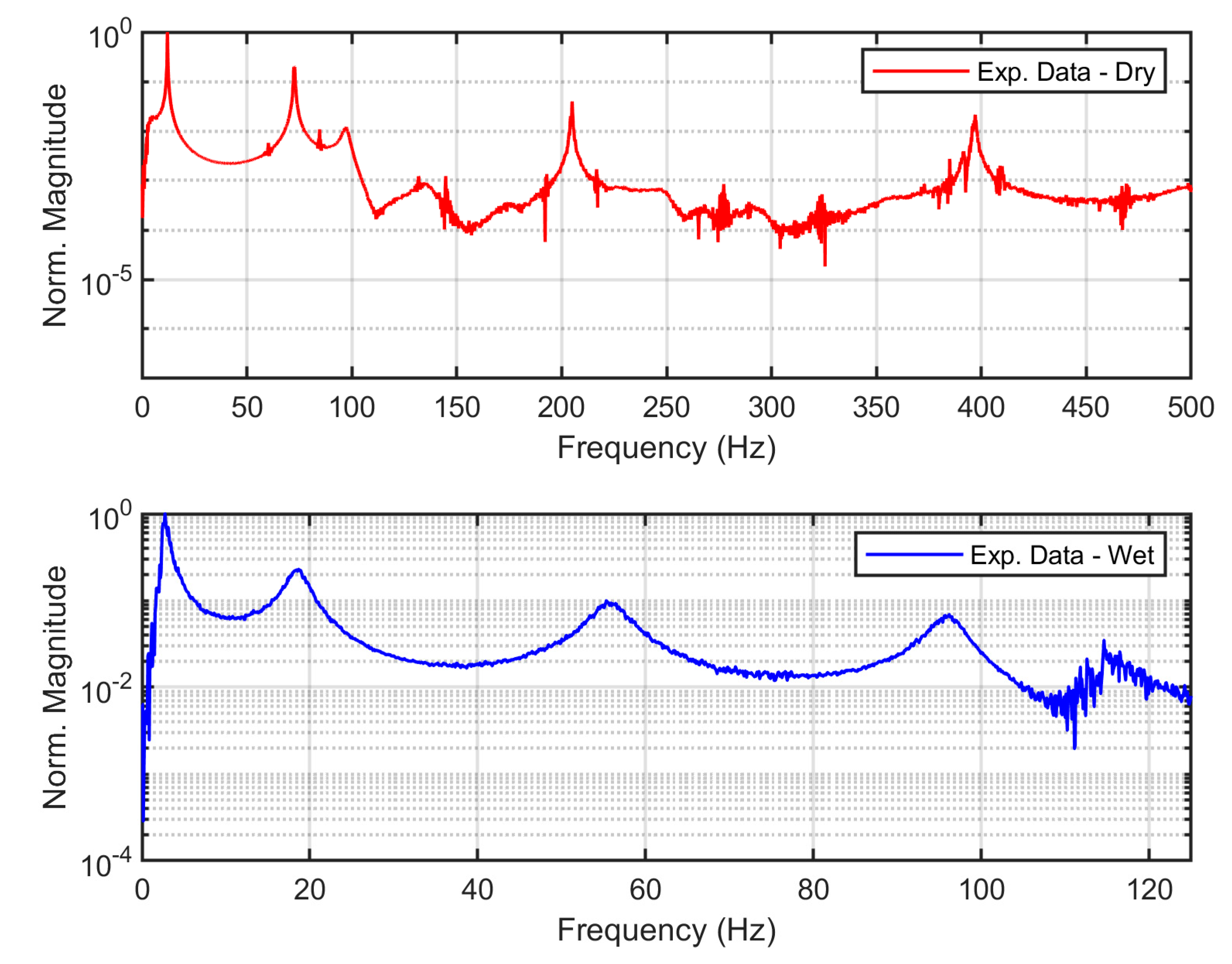
The natural frequencies are important characteristics where an error from this estimation would create discrepancies in all analyses. To extract natural frequencies of the beam from experiment, the shaker is driven by a random input signal from a signal generator. Both the signal generator and the signal analyser are provided by SignalCalc Ace powered by the Quattro hardware platform. The output signal from Quattro is amplified by an amplifier provided by LDS PA25E to meet the power required by the shaker. The output voltages from the laser vibrometer and accelerometer are connected to a signal analyser to estimate the frequency response function (FRF) using the fast Fourier transform (FFT) spectrum analysis. Thus, the FRF is the magnitude of the transfer function of the beam velocity from the laser vibrometer relative to the base acceleration. Figure 17 shows the FRF for the dry and wet models indicated with the red and blue lines, respectively.
The corresponding natural frequencies are indicated with local maxima at a certain range of frequencies. There are four peaks under 500 Hz for the dry model, while the same peaks appear in just up to 125 Hz for the wet model. The first mode shifts almost 9 Hz downward due to the influence of the added mass, M , which contributes about 1733% to the linear mass of the beam, μ . On the other hand, the undamped natural frequency from the analytical model can be derived from the stiffness over the mass per unit length from Equation (20) to give,
ω n 2   =   E I β n 4 ( μ + M ) L 4
where, in the case of clamped-free beam, β n / L is 1.875, 4.694, 7.855 and 10.996 for n = 1 , , 4 [26].
The comparison between analytical and experimental data is presented in Table 1. The error is calculated by subtracting the two values and dividing the result by the experiment data. Overall, the errors show less than 5% in the dry model indicating that the physical model is well approximated by the analytical approach. In the wet model, the first and fourth modes have good agreement with an error less than 4%, although there are some notable discrepancies, particularly in the second and third modes.
To investigate these phenomena, the FRF tests were conducted by measuring the base velocity to the input signal from the signal generator as shown in Figure 18. The first test indicated with the blue line was performed with the shaker in the unloaded condition (without the base), while the second test, the red line, was carried out with the beam and its base mounted on the shaker. Thus, the normalised magnitude in Figure 18 represents the transfer function of the base acceleration of the shaker relative to the signal generator with respect to frequency. It is seen from the figure that the natural frequency of the shaker appears around 47 Hz for the unloaded condition, while the peak displaces to 30 Hz due to the additional masses from the base, extension and beam on the shaker. The presence of this peak is due to the design of the shaker that uses spring components to hold the moving part [42,43]. Consequently, it tends to move the modes of the beam away from its origin, resulting in a noticeable error in the validation [44].

5.3. Discussion

In order to obtain the response of the analytical model, the linear, C i , and quadratic damping functions, C f , must first be determined. The combination of these damping functions can be approximated by using the Harmonic Balance method to give [45],
C q   =   C i + 8 C f ω n 3 π W
where C q is the equivalent damping and W is the maximum displacement amplitude or, in this case, the displacement envelope. Therefore, the constants C i and C f can be extracted from experiments by fitting the first order polynomial to the damping data with respect to the instantaneous displacement amplitude. In this case, we use the first decomposed signal of the experiment data presented in Figure 12a where it shows a clear decaying oscillation. The velocity time series is integrated numerically to obtain the displacement. If this procedure generates a peak at zero frequency, it means that the signal average is non-zero over the temporal window considered. In other words, the displacement response does not oscillate around zero. To centre the oscillation, a filter is applied in the frequency domain to bring the amplitude at zero frequency to zero. The filtered displacement is obtained by using the FFT inverse method.
The same procedures were applied to obtain the instantaneous vibration properties. The damping, C q , can be expressed by utilising the estimated damping ratio, ζ ( t ) , and the instantaneous frequency, f ( t ) , to give
C q   =   2 ζ ( t ) ( μ + M ) 2 π f ( t )
The result from Equation (25) is then plotted with respect to the displacement amplitude as presented in Figure 19. From the figure, the blue line from the figure shows the curve fitting of the experiment data to the first degree polynomial. It is seen from the figure that the linear regression generates a satisfactory fit indicated with the R-Square of 91.4%. Therefore, the constant C i and C f can be obtained by using the linear equation shown in Figure 19 which gives C i = 0.65 and C f = 33.0 . Following the procedure presented in [14,21], the quadratic damping values are estimated by
C f   =   1 2 ρ C d H
where H is the beam width, and C d is the drag coefficient which has the value of 1.8 for the flat plate model [46]. Substituting the parameters into Equation (26) would results in C f = 11.4 . Surprisingly, the damping value from this evaluation is underestimated compared to that of the experimental model. This is the reason why the analytical damping assumptions should be considered valid only for a small range of frequencies.
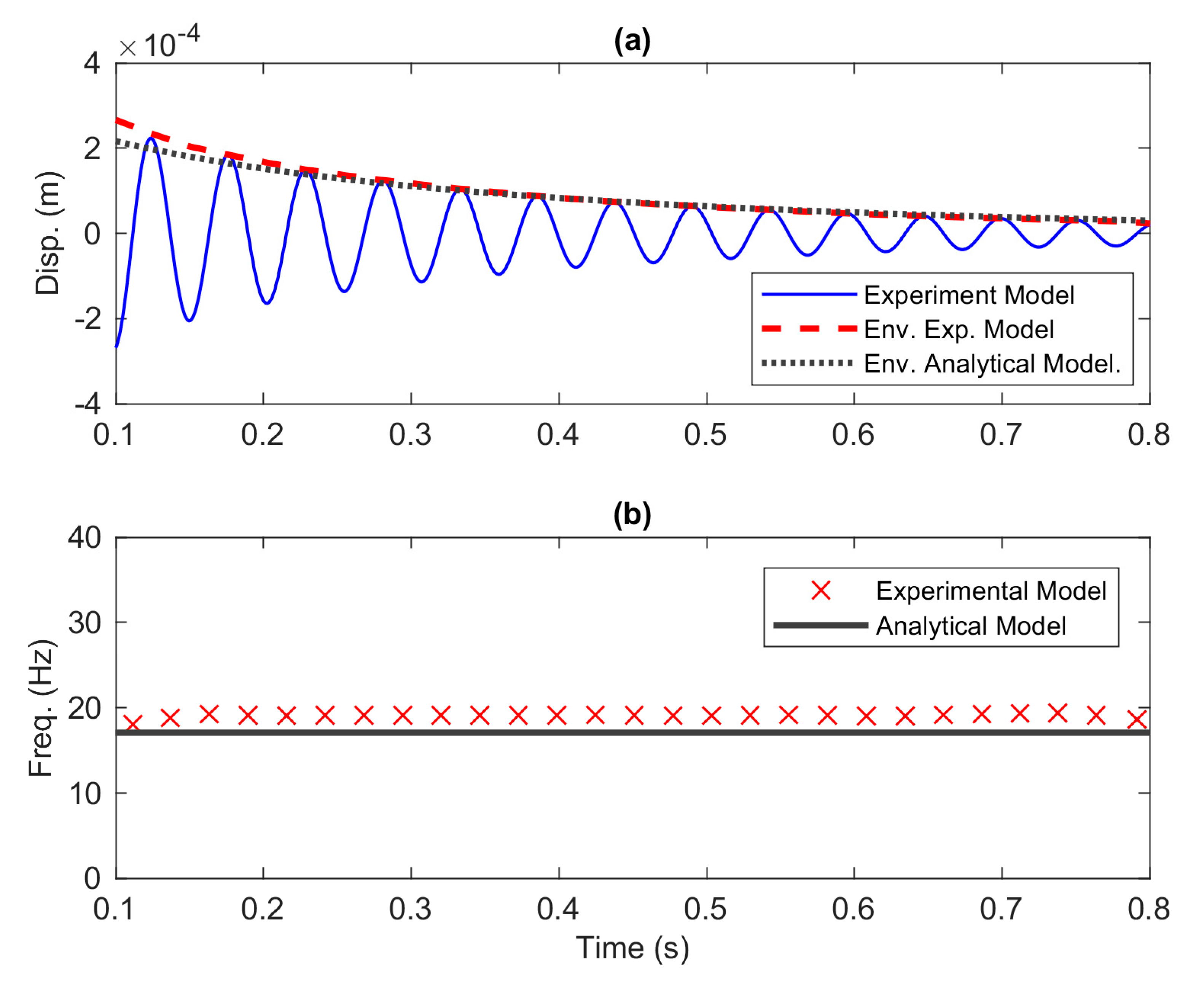
To obtain the dynamics of the responses of the beam, the damping coefficients from the fitting process are preferred to Equation (20). Figure 20a depicts the comparison of the instantaneous amplitude of the analytical model compared to that of the experimental model. It is seen from the figure that the envelope of the analytical model is capable of tracking the peaks of the experiment model over time. Figure 20b displays the time series of the instantaneous frequency for both the analytical and experiment models. The cause of the discrepancy between the two models was discussed in detail in the validation of natural frequencies, Section 5.2.
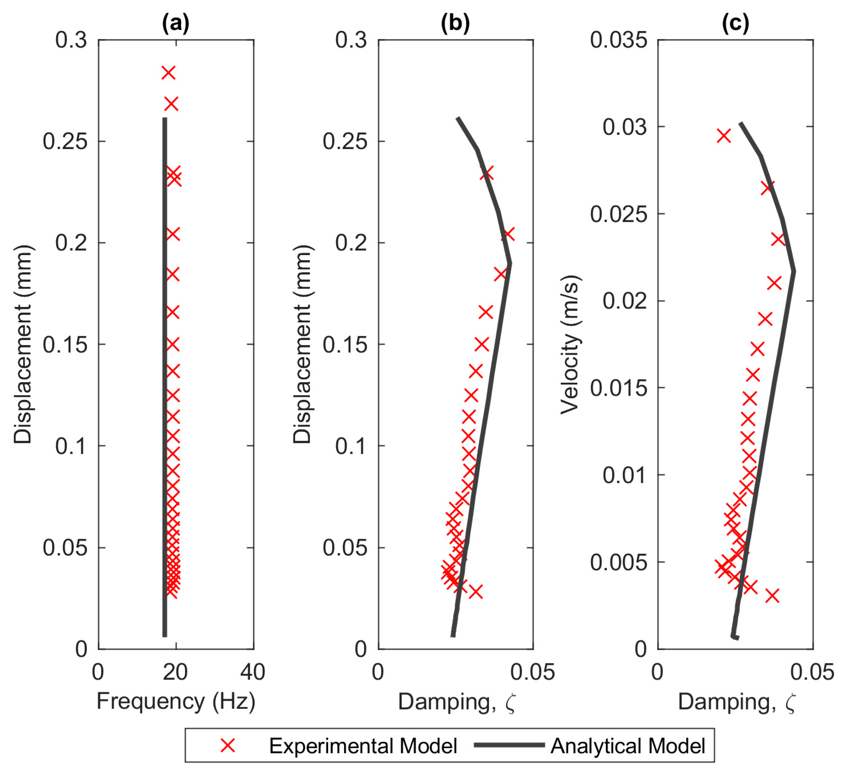
By pairing the instantaneous amplitude with the instantaneous frequency, the backbone curve can be constructed as illustrated in Figure 21a. The damping curves with respect to displacement and velocity amplitudes are depicted in Figure 21b,c, respectively. Overall, the analytical model can produce good agreement for predicting the dynamic behaviour of the structure in a fluid environment. One might expect the damping curves from the analytical model pass through the experimental data as illustrated in Figure 19. This is unlikely to occur due to the discrepancy in the natural frequencies between the two models where the damping ratio is inversely proportional to the resonant frequency based on Equation (25).

6. Conclusions

The method presented here has enabled the computation of backbone and damping curves of a fluid-structure interaction system particularly in the case of a beam immersed in liquid. All models agree that the backbone curve showing the natural frequencies of the system are linear. The damping curves from the experiments are successfully fitted with a first-degree polynomial equation which represents a combination of linear and quadratic damping models. The analytical models also demonstrate satisfactory performance using the damping computed from the experiments. However, the theoretical damping (Equation (26)) is significantly lower than that of the experiments. This is an indication that the theoretical damping estimation is only valid away from resonance. The numerical models on the other hand, overestimate the damping value when compared with the experimental results. For instance, at the instantaneous amplitude of 0.014 m/s, the numerical model generates a damping ratio of 0.248, while the experimental data only show a damping ratio of 0.03. Since this study only considers damping estimation at the tip of the beam and only some modes can be extracted from the responses, future work will focus on conducting nonlinear modal analysis that can cover several modes and evaluate the damping at various length.

Author Contributions

Conceptualization, S.N.H.S., H.Z.-B. and A.C.; methodology, S.N.H.S. and A.C.; software, S.N.H.S. and H.Z.B.; validation, S.N.H.S.; formal analysis, S.N.H.S. and H.Z.B.; investigation, S.N.H.S. and A.C.; resources, H.Z.-B. and A.C.; data curation, S.N.H.S.; writing—original draft preparation, S.N.H.S.; writing—review and editing, S.N.H.S., H.Z.-B. and A.C.; visualization, S.N.H.S.; supervision, H.Z.B. and A.C. All authors have read and agreed to the published version of the manuscript.

Funding

This research received no external funding.

Conflicts of Interest

The authors declare no conflict of interest.

References

  1. Avirovik, D.; Malladi, V.V.N.S.; Priya, S.; Tarazaga, P.A. Theoretical and experimental correlation of mechanical wave formation on beams. J. Intell. Mater. Syst. Struct. 2016, 27, 1939–1948. [Google Scholar] [CrossRef]
  2. Mashimo, T. Miniature preload mechanisms for a micro ultrasonic motor. Sens. Actuators A Phys. 2017, 257, 106–112. [Google Scholar] [CrossRef]
  3. Ramananarivo, S.; Godoy-Diana, R.; Thiria, B. Passive elastic mechanism to mimic fish-muscle action in anguilliform swimming. J. R. Soc. Interface 2013, 10. [Google Scholar] [CrossRef] [PubMed] [Green Version]
  4. Liu, G.; Zhang, W. Travelling-Wave Micropumps. In Micro Electro Mechanical System; Micro/Nano Technologies; Springer: Singapore, 2017; Volume 2, pp. 1–19. [Google Scholar] [CrossRef]
  5. Ye, W.; Liu, G.; Wang, C.; Li, W.; Yue, Z.; Zhang, W. Travelling wave magnetic valveless micropump driven by rotating integrated magnetic arrays. Micro AMP Nano Lett. 2014, 9, 232–234. [Google Scholar] [CrossRef]
  6. Zhang, W.; Wang, C.; Yue, Z.; Zhan, C.N.; Geng, W.D.; Liu, G.H. Travelling-wave piezoelectric micropump with low resistance microchannel. Electron. Lett. 2011, 47. [Google Scholar] [CrossRef]
  7. Ghommem, M.; Najar, F.; Arabi, M.; Abdel-Rahman, E.; Yavuz, M. A unified model for electrostatic sensors in fluid media. Nonlinear Dyn. 2020. [Google Scholar] [CrossRef]
  8. Shabani, R.; Hatami, H.; Golzar, F.G.; Tariverdilo, S.; Rezazadeh, G. Coupled vibration of a cantilever micro-beam submerged in a bounded incompressible fluid domain. Acta Mech. 2012, 224, 841–850. [Google Scholar] [CrossRef]
  9. Benra, F.-K.; Dohmen, H.J.; Pei, J.; Schuster, S.; Wan, B. A Comparison of One-Way and Two-Way Coupling Methods for Numerical Analysis of Fluid-Structure Interactions. J. Appl. Math. 2011, 2011, 1–16. [Google Scholar] [CrossRef]
  10. Erturk, A.; Delporte, G. Underwater thrust and power generation using flexible piezoelectric composites: An experimental investigation toward self-powered swimmer-sensor platforms. Smart Mater. Struct. 2011, 20. [Google Scholar] [CrossRef]
  11. Jeong, Y.D.; Lee, J.H. Passive locomotion of freely movable flexible fins near the ground. J. Fluids Struct. 2018, 82, 1–15. [Google Scholar] [CrossRef]
  12. Koushesh, A. Added Mass Formulation for Fluid-Structure Interaction. Master’s Thesis, American University of Sarjah, Sarjah, UAE, 2016. [Google Scholar]
  13. Xiu, H.; Davis, R.B.; Romeo, R.C. Edge clearance effects on the added mass and damping of beams submerged in viscous fluids. J. Fluids Struct. 2018, 83, 194–217. [Google Scholar] [CrossRef]
  14. Kaneko, S.; Nakamura, T.; Inada, F.; Kato, M.; Ishihara, K.; Nishihara, T.; Mureithi, N.; Langthjem, M. Flow-Induced Vibrations, 2nd ed.; Academic Press: Cambridge, UK, 2014. [Google Scholar] [CrossRef]
  15. Païdoussis, M.P. Fluid-Structure Interactions, 2nd ed.; Slender Structures and Axial Flow; Academic Press: Cambridge, UK, 2016; Volume 2. [Google Scholar] [CrossRef]
  16. Taylor, G.I. Analysis of the swimming of long and narrow animals. Proc. R. Soc. Lond. Ser. A Math. Phys. Sci. 1952, 214, 158–183. [Google Scholar] [CrossRef]
  17. Hatami, H.; Bagheri, A.; Ansari, R. An Analytical Investigation for Vibration Characteristics of a Beam-Type Liquid Micro-Pump. Int. J. Appl. Mech. 2020, 12. [Google Scholar] [CrossRef]
  18. Hou, J.; Wang, H.; Xu, D.; Jankowski, Ł.; Wang, P. Damage Identification Based on Adding Mass for Liquid–Solid Coupling Structures. Appl. Sci. 2020, 10, 2312. [Google Scholar] [CrossRef] [Green Version]
  19. Piñeirua, M.; Godoy-Diana, R.; Thiria, B. Resistive thrust production can be as crucial as added mass mechanisms for inertial undulatory swimmers. Phys. Rev. E 2015, 92. [Google Scholar] [CrossRef] [Green Version]
  20. Cen, L.; Erturk, A. Bio-inspired aquatic robotics by untethered piezohydroelastic actuation. Bioinspir. Biomim. 2013, 8. [Google Scholar] [CrossRef] [Green Version]
  21. Ramananarivo, S.; Godoy-Diana, R.; Thiria, B. Propagating waves in bounded elastic media: Transition from standing waves to anguilliform kinematics. EPL 2014, 105. [Google Scholar] [CrossRef]
  22. Kohtanen, E.A.; Davis, R.B. Hydroelastic damping of low aspect ratio cantilevered plates. J. Fluids Struct. 2019, 90, 315–333. [Google Scholar] [CrossRef]
  23. Shahab, S.; Tan, D.; Erturk, A. Hydrodynamic thrust generation and power consumption investigations for piezoelectric fins with different aspect ratios. Eur. Phys. J. Spec. Top. 2015, 224, 3419–3434. [Google Scholar] [CrossRef]
  24. Monette, C.; Nennemann, B.; Seeley, C.; Coutu, A.; Marmont, H. Hydro-dynamic damping theory in flowing water. IOP Conf. Ser. Earth Environ. Sci. 2014, 22. [Google Scholar] [CrossRef]
  25. Wang, Y.; Masoumi, M.; Gaucher-Petitdemange, M. Damping analysis of a flexible cantilever beam containing an internal fluid channel: Experiment, modeling and analysis. J. Sound Vib. 2015, 340, 331–342. [Google Scholar] [CrossRef]
  26. Inman, D.J. Engineering Vibrations, 4th ed.; Pearson: Hong Kong, China, 2013. [Google Scholar]
  27. Rao, S.S. Mechanical Vibration, 5th ed.; Pearson: Hong Kong, China, 2010. [Google Scholar]
  28. Hosoya, N.; Kajiwara, I.; Umenai, K.; Maeda, S. Dynamic characterizations of underwater structures using noncontact vibration tests based on nanosecond laser ablation in water: Evaluation of passive vibration suppression with damping materials. J. Vib. Control 2017, 24, 3714–3725. [Google Scholar] [CrossRef]
  29. Vu, V.H.; Thomas, M.; Lakis, A.A.; Marcouiller, L. Effect of Added Mass on Submerged Vibrated Plates. In Proceedings of the 25th Seminar on Machinery Vibration; Canadian Machinery Vibration Association (CMVA 7): Saint John, NB, Canada, 2007; pp. 40–41. [Google Scholar]
  30. Liu, X.; Luo, Y.; Karney, B.W.; Wang, Z.; Zhai, L. Virtual testing for modal and damping ratio identification of submerged structures using the PolyMAX algorithm with two-way fluid–structure Interactions. J. Fluids Struct. 2015, 54, 548–565. [Google Scholar] [CrossRef]
  31. Londoño, J.M.; Neild, S.A.; Cooper, J.E. Identification of backbone curves of nonlinear systems from resonance decay responses. J. Sound Vib. 2015, 348, 224–238. [Google Scholar] [CrossRef] [Green Version]
  32. Naylor, S.; Platten, M.F.; Wright, J.R.; Cooper, J.E. Identification of Multi-Degree of Freedom Systems With Nonproportional Damping Using the Resonant Decay Method. J. Vib. Acoust. 2004, 126, 298–306. [Google Scholar] [CrossRef]
  33. Feldman, M. Time-varying vibration decomposition and analysis based on the Hilbert transform. J. Sound Vib. 2006, 295, 518–530. [Google Scholar] [CrossRef]
  34. Feldman, M. Hilbert transform in vibration analysis. Mech. Syst. Signal. Process. 2011, 25, 735–802. [Google Scholar] [CrossRef]
  35. Feldman, M. Hilbert Transform. Applications in Mechanical Vibration; Wiley: Hoboken, NJ, USA, 2011. [Google Scholar] [CrossRef]
  36. Sumali, H.; Kellog, R.A. Calculating Damping from Ring-Down Using Hilbert Transform and Curve Fitting. In Proceedings of the 4th International Operational Modal Analysis Conference (IOMAC), Istanbul, Turkey, 9–11 May 2011. [Google Scholar]
  37. Rao, S.S. Vibration of Continuous Systems, 2nd ed.; John Wiley & Sons, Inc.: Hoboken, NJ, USA, 2007. [Google Scholar]
  38. Bachmann, H.; Ammann, W.J.; Deischl, F.; Eisenmann, J.; Floegl, I.; Hirsch, G.H.; Klein, G.K.; Lande, G.J.; Mahrenholtz, O.; Natke, H.G.; et al. Vibration Problems in Structures; Birkhäuser Basel: Basel, Switzerland, 1995. [Google Scholar] [CrossRef]
  39. Erturk, A.; Inman, D.J. An experimentally validated bimorph cantilever model for piezoelectric energy harvesting from base excitations. Smart Mater. Struct. 2009, 18. [Google Scholar] [CrossRef]
  40. Erturk, A.; Inman, D.J. On Mechanical Modeling of Cantilevered Piezoelectric Vibration Energy Harvesters. J. Intell. Mater. Syst. Struct. 2008, 19, 1311–1325. [Google Scholar] [CrossRef]
  41. Wagg, D.; Neild, S. Nonlinear Vibration with Control: For Flexible and Adaptive Structures, 2nd ed.; Springer International Publishing: Cham, Switzerland, 2015. [Google Scholar] [CrossRef]
  42. Hoffait, S.; Marin, F.; Simon, D.; Peeters, B.; Golinval, J.-C. Measured-based shaker model to virtually simulate vibration sine test. Case Stud. Mech. Syst. Signal. Process. 2016, 4, 1–7. [Google Scholar] [CrossRef] [Green Version]
  43. Tiwari, N.; Puri, A.; Saraswat, A. Lumped parameter modelling and methodology for extraction of model parameters for an electrodynamic shaker. J. Low Freq. Noise Vib. Act. Control. 2017, 36, 99–115. [Google Scholar] [CrossRef]
  44. Syuhri, S.N.H.; McCartney, A.; Cammarano, A. Development of an Experimental Rig for Emulating Undulatory Locomotion. In Nonlinear Structures & Systems, Proceedings of the Society for Experimental Mechanics Series, IMAC XXXVII, Houston, TX, USA, 10–13 February 2020; Springer: Cham, Switzerland, 2020; Volume 1, pp. 253–263. [Google Scholar] [CrossRef]
  45. Mezghani, F.; Del Rincón, A.F.; Souf, M.A.B.; Fernandez, P.G.; Chaari, F.; Viadero Rueda, F.; Haddar, M. Identification of nonlinear anti-vibration isolator properties. Comptes Rendus Mécanique 2017, 345, 386–398. [Google Scholar] [CrossRef]
  46. Buchak, P.; Eloy, C.; Reis, P.M. The Clapping Book: Wind-Driven Oscillations in a Stack of Elastic Sheets. Phys. Rev. Lett. 2010, 105. [Google Scholar] [CrossRef] [PubMed] [Green Version]
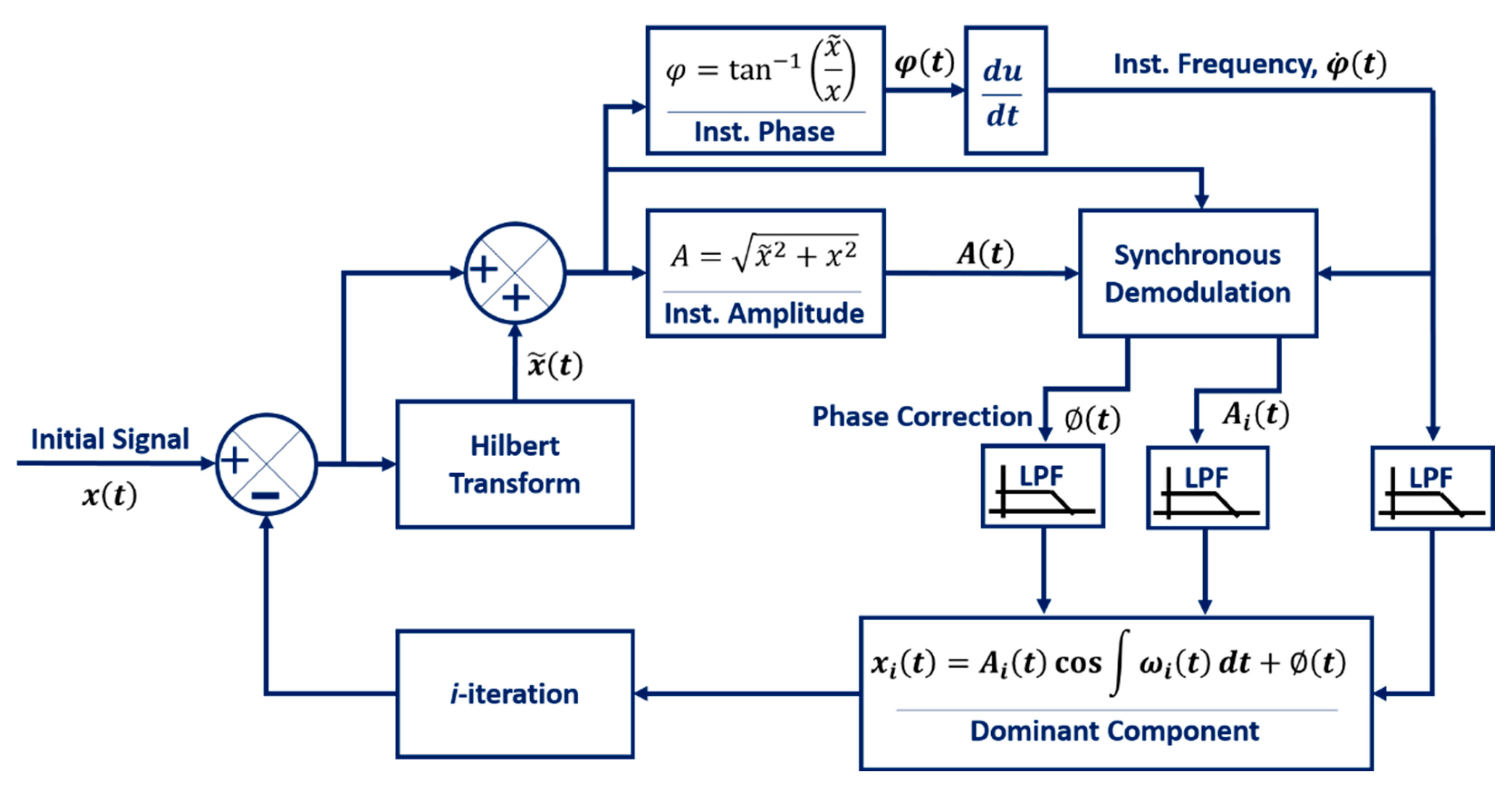
Figure 1. The HVD procedure for extracting a multicomponent vibratory signal.
Vibration 03 00032 g001
Figure 2. A typical response of an underdamped system.
Vibration 03 00032 g002
Figure 3. Cantilevered beam immersed in a liquid excited by the translation of its base.
Vibration 03 00032 g003
Figure 4. Cantilevered beam immersed in a liquid excited by the translation of its base.
Vibration 03 00032 g004
Figure 5. (a) The time series of velocity at x = 8 cm, and the 3D plot of velocity in various frequency and beam length of (b) the experimental model and (c) the numerical model.
Vibration 03 00032 g005
Figure 6. The decomposed signals of the (a) experiment data and (b) numerical data.
Vibration 03 00032 g006
Figure 7. Backbone curves of (a) the first and (b) second modes.
Vibration 03 00032 g007
Figure 8. Damping curves of (a) the first and (b) second modes.
Vibration 03 00032 g008
Figure 9. (a) The time series of velocity at x = 8 cm and the frequency series of (b) the experimental model and (c) the numerical model.
Vibration 03 00032 g009
Figure 10. The decomposed signals of (a) the experiment model and (b) the numerical model.
Vibration 03 00032 g010
Figure 11. (a) The time series of velocity at x = 8 cm and the frequency series of (b) the experimental model and (c) the numerical model.
Vibration 03 00032 g011
Figure 12. The decomposed signals of (a) the experiment model and (b) the numerical model.
Vibration 03 00032 g012
Figure 13. (a) Time series of the velocity at the tip of the beam, (b) velocity amplitude vs. frequency at several locations along the beam, and (c) time series of the first and second decomposed signals.
Vibration 03 00032 g013
Figure 14. Time series of frequency.
Vibration 03 00032 g014
Figure 15. The backbone curves estimated from the envelope of (a) the first mode of numerical models, (b) the second mode and (c) the third mode of the experimental models.
Vibration 03 00032 g015
Figure 16. The damping curves extracted from, (a,b) the numerical models and (c) the experimental models.
Vibration 03 00032 g016
Figure 17. FRF of the beam in dry and wet conditions.
Vibration 03 00032 g017
Figure 18. Frequency response of the base velocity relative to the input signal generator.
Vibration 03 00032 g018
Figure 19. The curve fitting method to obtain the damping coefficients.
Vibration 03 00032 g019
Figure 20. The time series of (a) displacement and (b) frequency.
Vibration 03 00032 g020
Figure 21. (a) The backbone curve, and the damping curves with respect to (b) displacement and (c) velocity.
Vibration 03 00032 g021
Table 1. Natural frequencies from analytical and experimental data.
Dry
Exp. (Hz)Calc. (Hz)Error (%)
12.031311.53284.1431
71.953172.27470.4469
202.2656202.37120.0522
393.7500396.56680.7154
Wet
Exp. (Hz)Calc. (Hz)Error (%)
2.73442.69351.4947
18.671916.87999.5972
55.312547.264214.5506
96.171992.61903.6943
Publisher’s Note: MDPI stays neutral with regard to jurisdictional claims in published maps and institutional affiliations.