
Deep Machine Learning for Acoustic Inspection of Metallic Medium


Abstract
:1. Introduction
1.1. Motivation
1.2. Theory
Frequency Domain Analysis
2. Materials and Methods
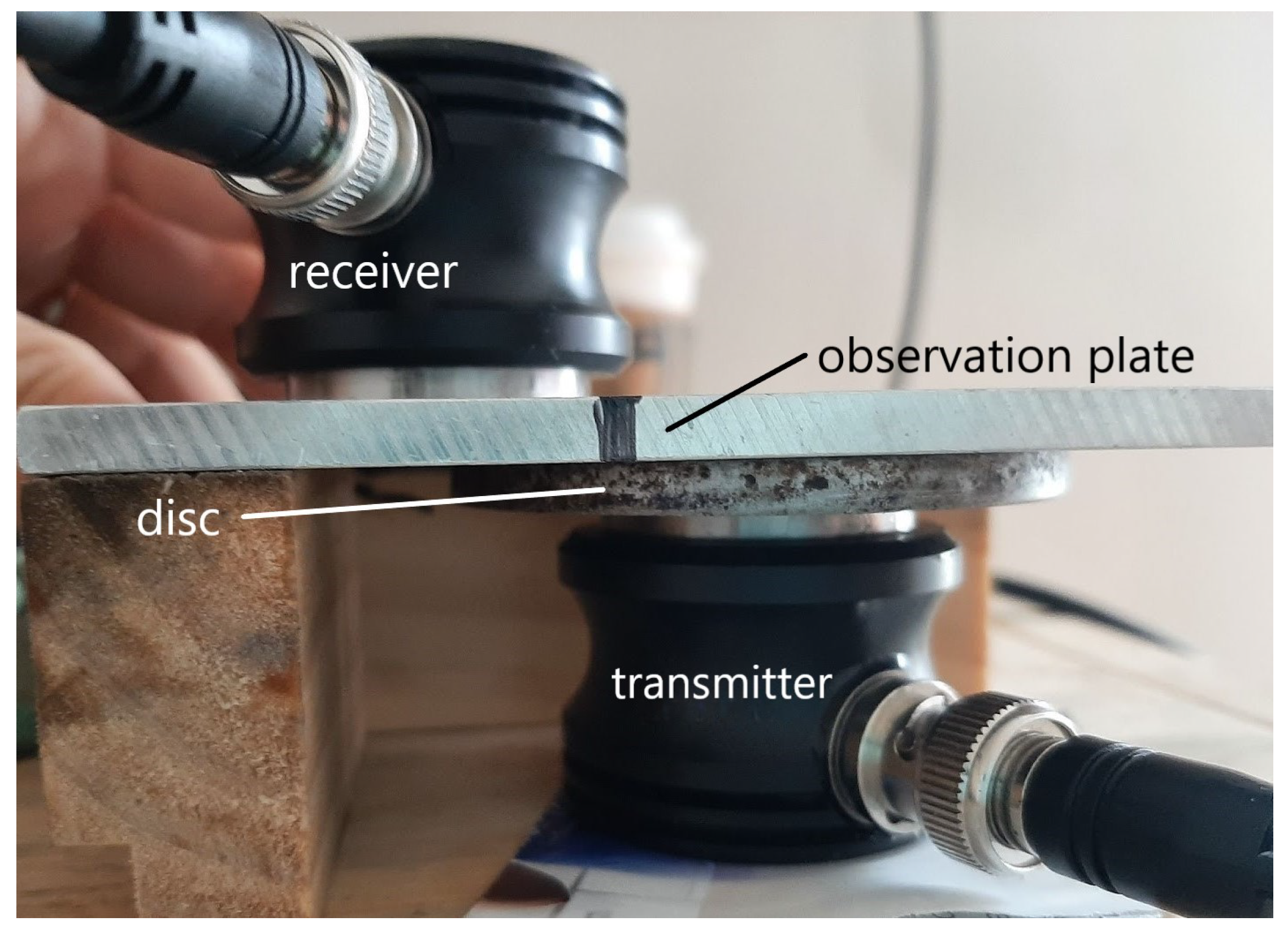
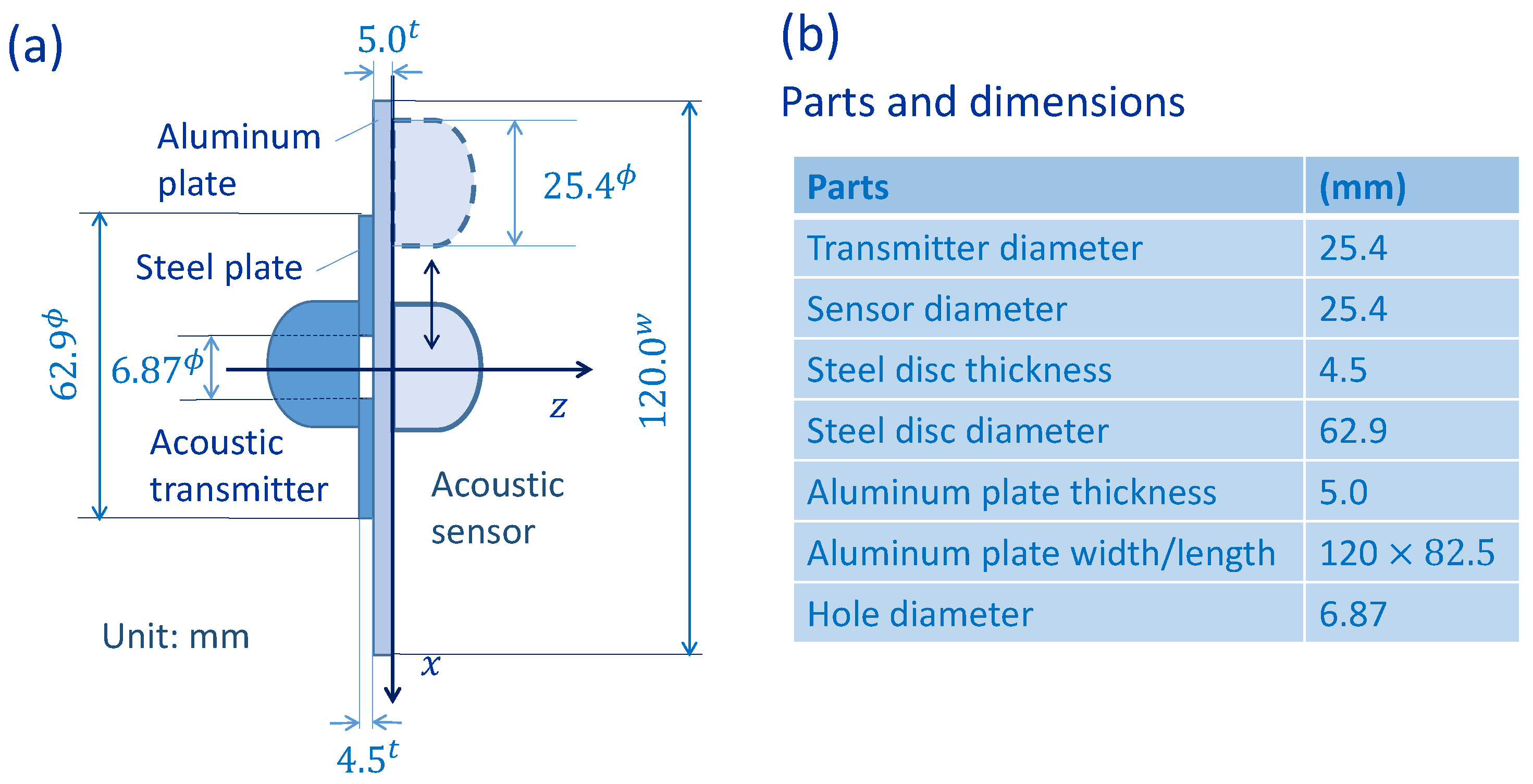
2.1. System Design and Data Collection
2.2. Preprocessing
2.3. Convolutional Neural Network
2.3.1. Background
2.3.2. Present Model
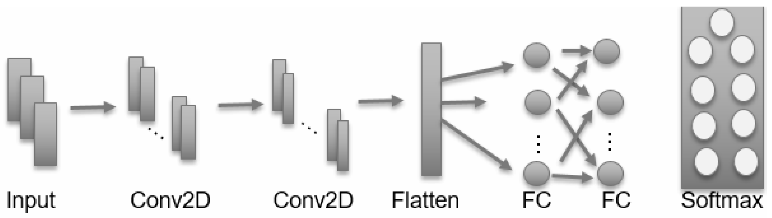
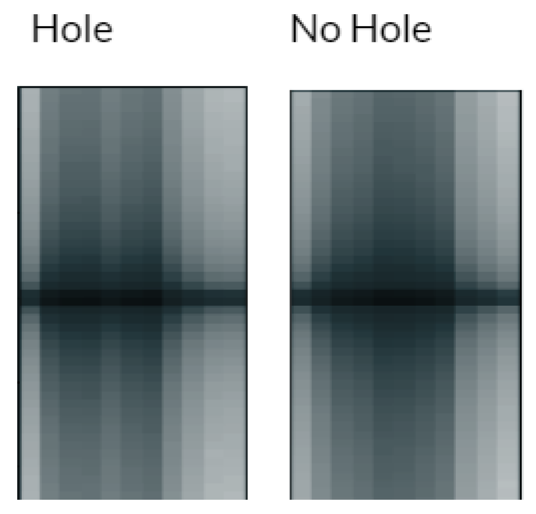
- Input: The CNN accepts images sized 200 × 15 × 1. These have been normalized between 0 and 1 and augmented with light noise to avoid overfitting. A sample of these input images can be seen in Figure 10. These images are expanded to increase visibility, but at the time they are fed to the CNN they have dimensions of 200 pixels in height and 15 pixels in width.
- Convolution Layers: For the first of these layers, convolution is performed with 64 filters. These filters have a 5 × 5 receptive field applied using a stride size of one. Finally, the ReLU activation function is applied to the feature maps. This feature map is then fed directly to the second of these layers where convolution is performed with 64 filters. These filters have a 3 × 3 receptive field applied using a stride size of one. Finally, the ReLU activation function is applied to the new feature maps.
- Flattening: This layer takes the feature maps which result from the first two convolution layers and flattens them into a one-dimensional vector. This vector is fed to the fully connected layers.
- Fully Connected Layers: In the first fully connected layer the flattened output is connected to 720 hidden units. Here the ReLU activation function is applied to produce the next feature vector. In this fully connected layer, the output is connected to only 80 hidden units. Again the ReLU activation function is applied to produce the feature vector which will be used by the final layer of the CNN. A dropout of 0.4 was applied to each fully connected layer to avoid overfitting the training data.
- Softmax: The softmax layer is a nine-dimensional vector that represents the probability of belonging to each of the nine labels.
3. Results
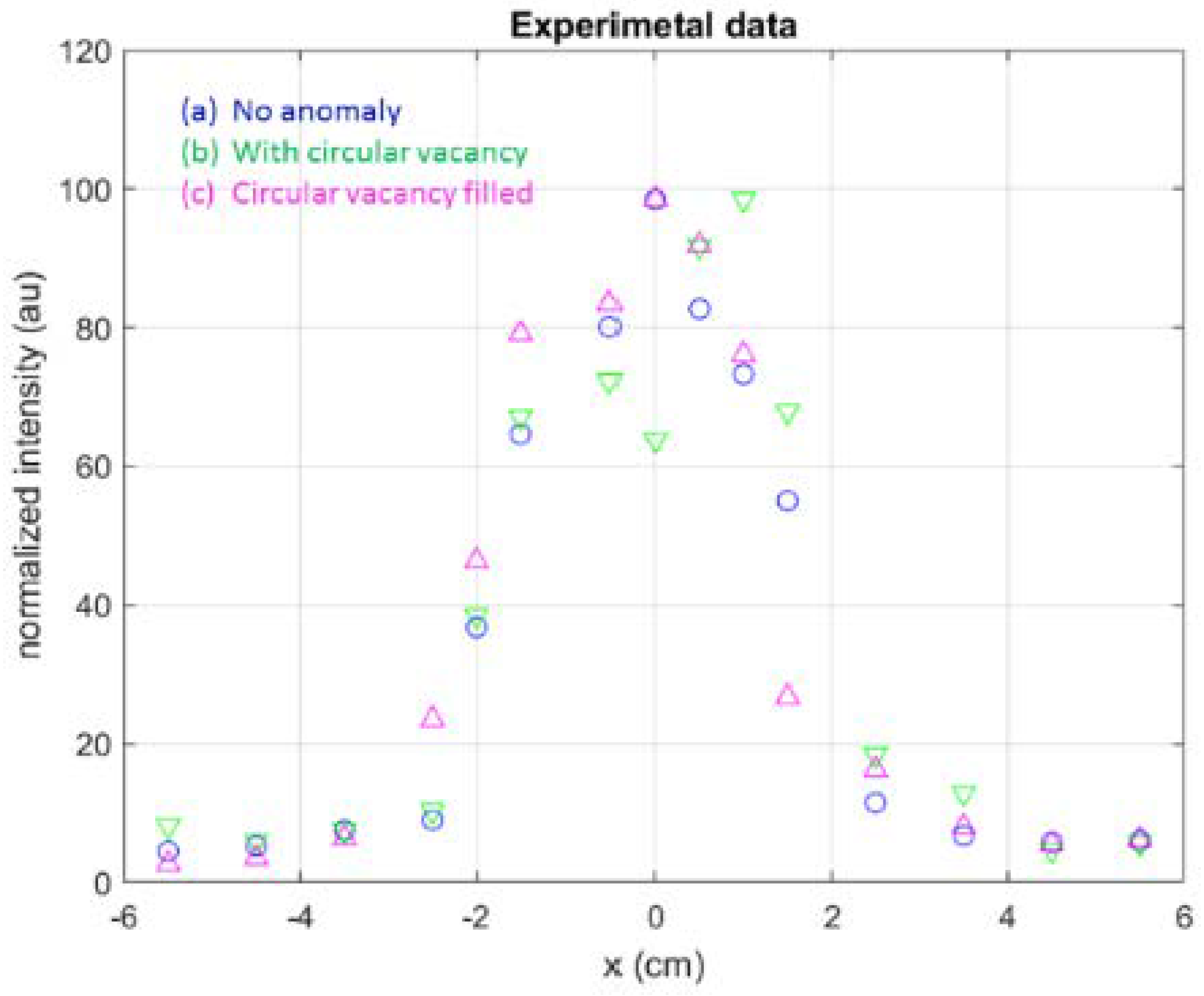
3.1. Results of Measurements
3.1.1. Time Domain Signals
3.1.2. Modal Analysis
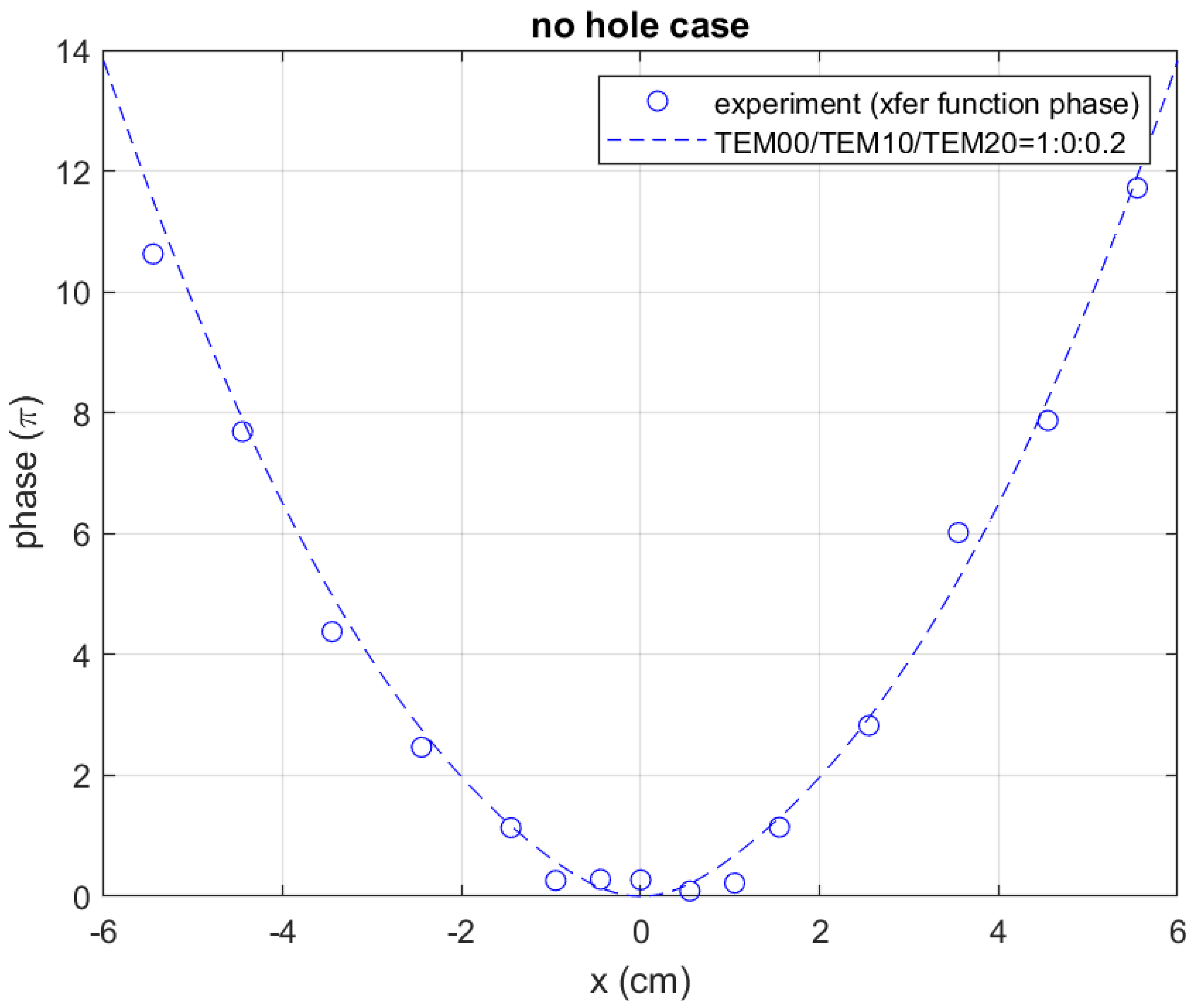
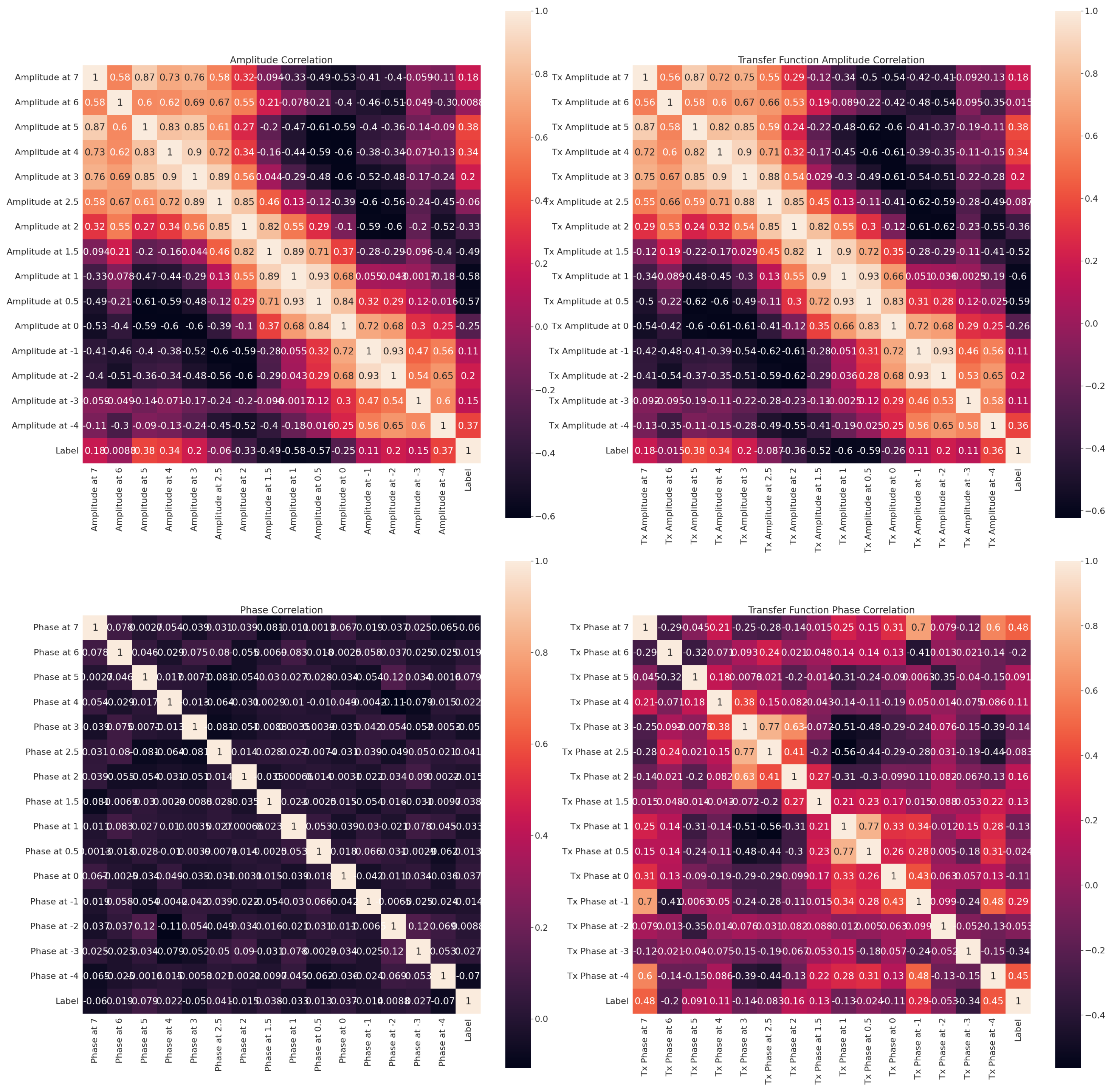
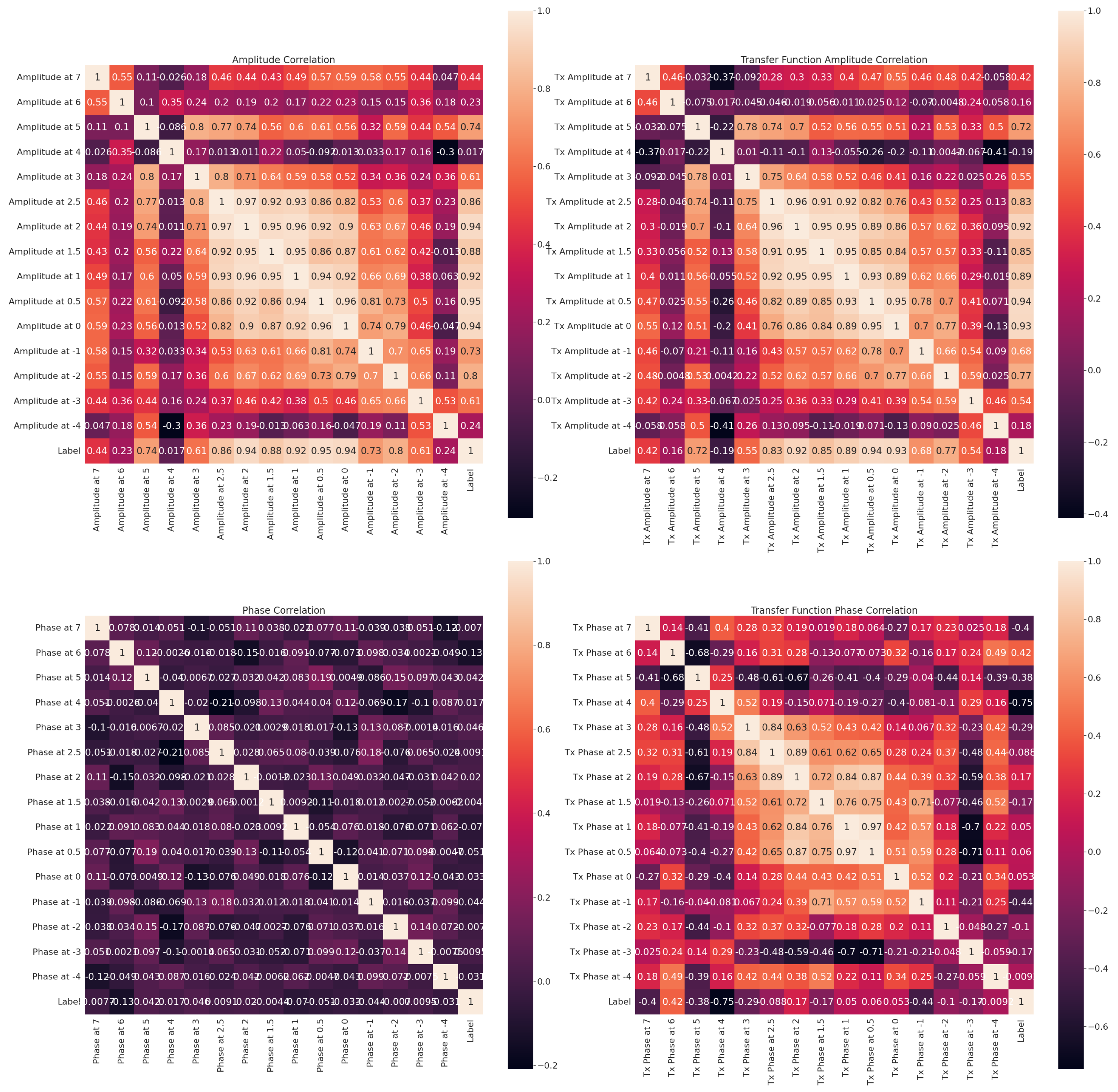
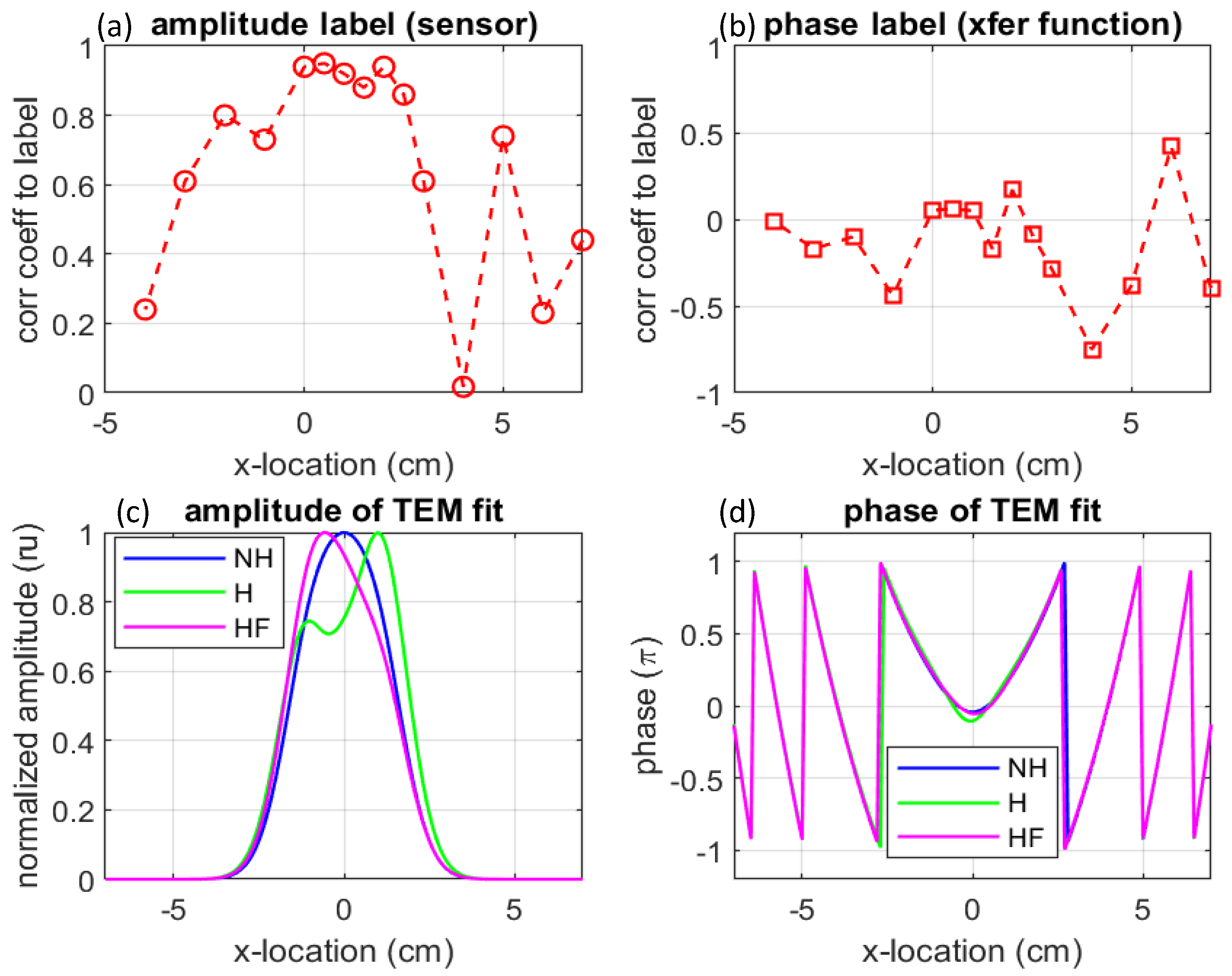
3.1.3. Amplitude and Phase of Sensor Signal and Transfer Function
3.2. Results of CNN
3.2.1. CNN Performance
3.2.2. K-Fold Validation
4. Discussion
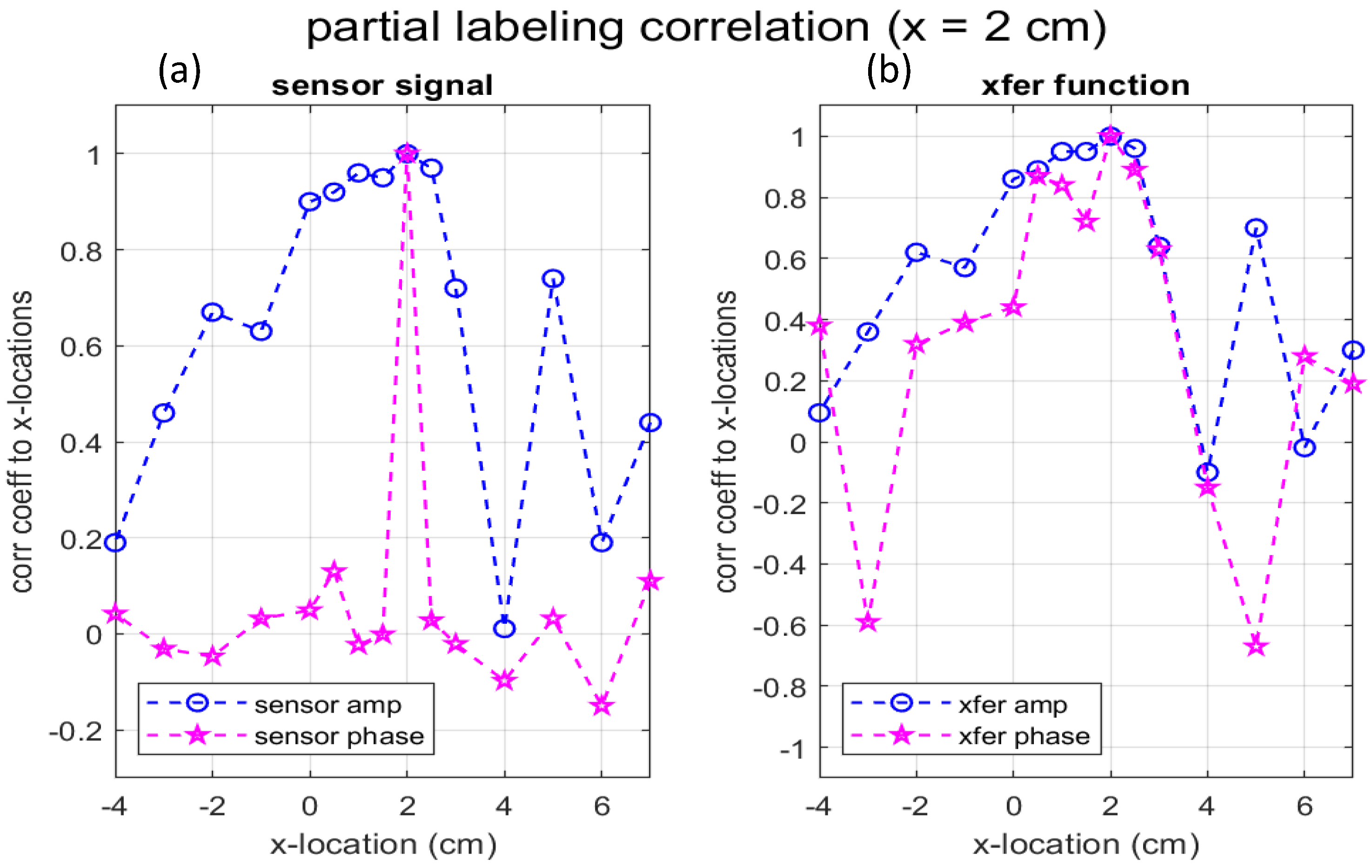
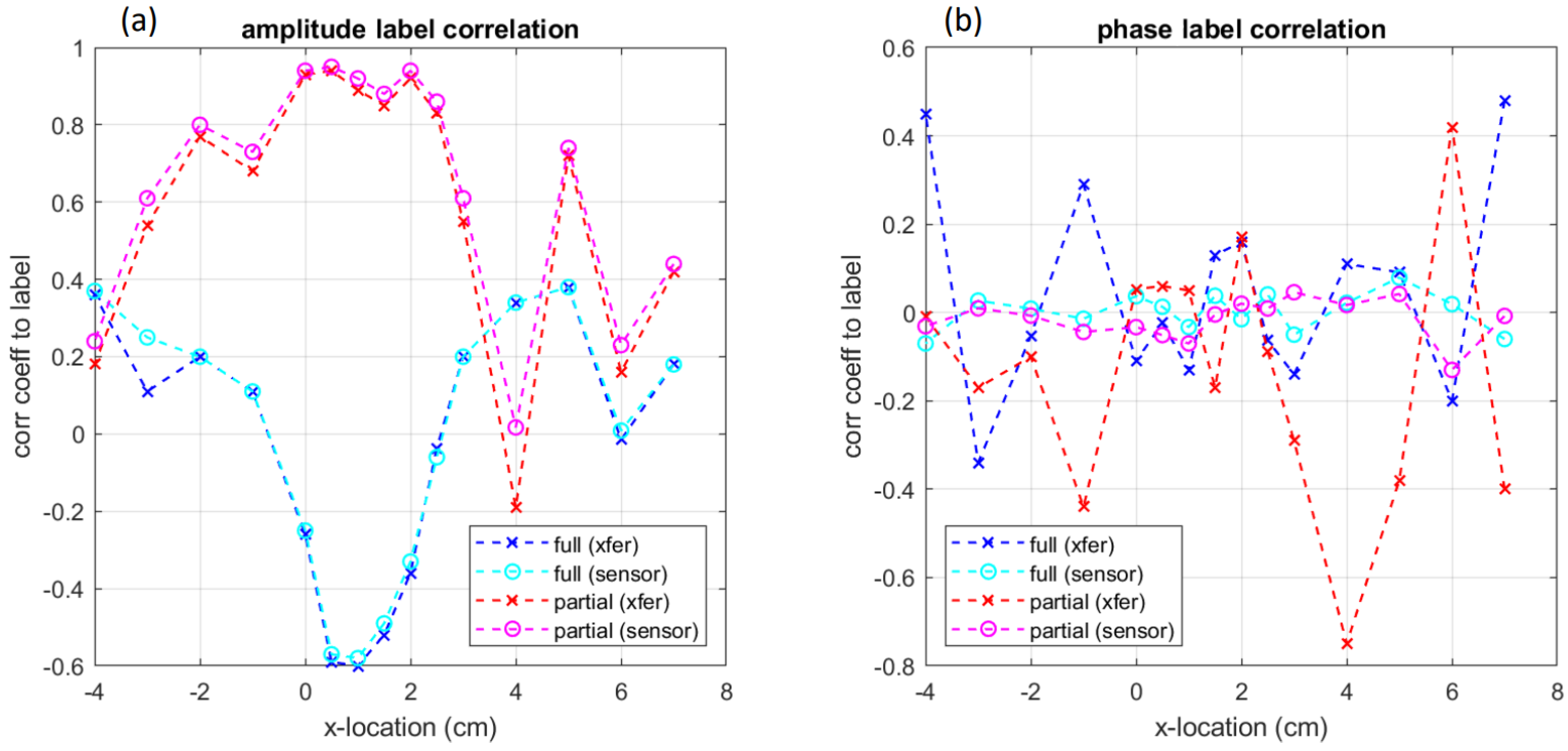
4.1. Correlation Analysis
4.2. Separability
5. Conclusions
Author Contributions
Funding
Institutional Review Board Statement
Informed Consent Statement
Data Availability Statement
Conflicts of Interest
Abbreviations
| CNN | Convolutional Neural Network |
| AE | Acoustic Emissions |
| FFT | Fast Fourier Transform |
| SDFT | Short Distance Fourier Transform |
References
- Graff, K.F. Wave Motion in Elastic Solids; Oxford Univ. Press: Oxford, UK, 1975. [Google Scholar]
- Krautkrämer, J.; Krautkrämer, H. Ultrasonic Testing of Materials; Springer: Berlin/Heidelberg, Germany, 1990. [Google Scholar]
- Drinkwater, B.W.; Wilcox, P.D. Ultrasonic arrays for non-destructive evaluation: A review. NDT & E Int. 2006, 39, 525–541. [Google Scholar]
- Zinin, P.V.; Arnold, W.; Weise, W.; Slabeyciusova-Berezina, S. Theory and Applications of Scanning Acoustic Microscopy and Scanning Near-Field Acoustic Imaging. In Ultrasonic and Electromagnetic NDE for Structure and Material Characterization, 1st ed.; Kundu, T., Ed.; CRC Press: Boca Raton, FL, USA, 2012; Chapter 11; pp. 611–688. [Google Scholar]
- Juntarapaso, Y.; Miyasaka, C.; Tutwiler, R.L.; Anastasiadis, P. Contrast Mechanisms for Tumor Cells by High-frequency Ultrasound. Open Neuroimaging J. 2018, 12, 105–119. [Google Scholar] [CrossRef]
- Ono, Y.; Kushibiki, J. Experimental study of construction mechanism of V(z) curves obtained by line-focus-beam acoustic microscopy. IEEE Trans. Ultrason. Ferroelectr. Freq. Control 2000, 47, 1042–1050. [Google Scholar] [CrossRef] [PubMed]
- Duquennoy, M.; Ourak, M.; Xu, W.J.; Nongaillard, B.; Ouaftouh, M. Observation of V(z) curves with multiple echoes. NDT Int. 1995, 28, 147–153. [Google Scholar] [CrossRef]
- Miyasaka, C.; Yoshida, S. Overview of Recent Advancement in Ultrasonic Imaging for Biomedical Applications. Open Neuroimaging J. 2018, 12, 133–157. [Google Scholar] [CrossRef]
- Miyaska, K.; Laprime, E.; Yoshida, S.; Sasaki, T. Application of Gaussian Beam to Ultrasonic Testing. In The Abstracts of ATEM: International Conference on Advanced Technology in Experimental Mechanics: Asian Conference on Experimental Mechanics; The Japan Society of Mechanical Engineers: Tokyo, Japan, 2019; p. 1008B1415. [Google Scholar]
- Hilderbrand, J.A.; Rugar, D.; Johnston, R.N.; Quate, C.F. Acoustic microscopy of living cells. Proc. Natl. Acad. Sci. USA 1981, 78, 1656–1660. [Google Scholar] [CrossRef]
- Mahesh, B. Application of Non-Destructive Testing in Oil and Gas Industries. Int. J. Res. Eng. Sci. Manag. 2020, 2, 613–615. [Google Scholar]
- Hover, F.S.; Eustice, R.M.; Kim, A.; Englot, B.; Johannsson, H.; Kaess, M.; Leonard, J.J. Advanced perception, navigation and planning for autonomous in-water ship hull inspection. Int. J. Robot. Res. 2012, 31, 1445–1464. [Google Scholar] [CrossRef]
- Anusha, R.; Subhashini, P.; Jyothi, D.; Harshitha, P.; Sushma, J.; Mukesh, N. Speech Emotion Recognition using Machine Learning. In Proceedings of the 2021 5th International Conference on Trends in Electronics and Informatics (ICOEI), Tirunelveli, India, 3–5 June 2021; pp. 1608–1612. [Google Scholar] [CrossRef]
- Xiang, Z.; Zhang, R.; Seeling, P. Machine learning for object detection. In Computing in Communication Networks; Academic Press: Cambridge, MA, USA, 2020; pp. 325–338. [Google Scholar]
- Richter, T.; Fishbain, B.; Markus, A.; Richter-Levin, G.; Okon-Singer, H. Using machine learning-based analysis for behavioral differentiation between anxiety and depression. Sci. Rep. 2020, 10, 16381. [Google Scholar] [CrossRef]
- Haile, M.A.; Zhu, E.; Hsu, C.; Bradley, N. Deep machine learning for detection of acoustic wave reflections. Struct. Health Monit. 2020, 19, 1340–1350. [Google Scholar] [CrossRef]
- Brownlee, J. A Gentle Introduction to Long Short-Term Memory Networks by the Experts. Available online: https://machinelearningmastery.com/gentle-introduction-long-short-term-memory-networks-experts/ (accessed on 11 June 2022).
- Barat, V.; Kostenko, P.; Bardakov, V.; Terentyev, D. Acoustic signals recognition by convolutional neural network. Int. J. Appl. Eng. Res. 2017, 12, 3461–3469. [Google Scholar]
- Zhao, J. Anomalous Sound Detection Based on Convolutional Neural Network and Mixed Features. J. Phys. Conf. Ser. 2020, 1621, 012025. [Google Scholar] [CrossRef]
- Smith, D.G. Ebook Topic: Huygens’ and Huygens-Fresnel Principles. In Field Guide to Physical Optics; SPIE: Bellingham, WA, USA, 2013. [Google Scholar]
- Guenther, B.D.; Steel, D. Encyclopedia of Modern Optics; Academic Press: Cambridge, MA, USA, 2018; p. 69. [Google Scholar]
- Zinin, P.V.; Arnold, W.; Weise, W.; Berezina, S. Ultrasonic and Electromagnetic NDE for Structure and Material Characterization, 1st ed.; Kundu, T., Ed.; CRC Press: Boca Raton, FL, USA, 2012; Chapter 11. [Google Scholar]
- Weise, W.; Zinin, P.; Briggs, A.; Wilson, T.; Boseck, S. Examination of the two-dimensional pupil function in coherent scanning microscopes using spherical particles. J. Acoust. Soc. Am. 1998, 104, 181–191. [Google Scholar] [CrossRef] [PubMed]
- Soskind, Y.G. Ebook Topic: Fresnel Diffraction. In Field Guide to Diffractive Optics; SPIE: Bellingham, WA, USA, 2011. [Google Scholar]
- Goodman, J.W. Introduction to Fourier Optics. In McGraw-Hill Physical and Quantum Electronics Series; Roberts & Company Publishers: Greenwood Village, CO, USA, 2005. [Google Scholar]
- Lippmann, G. Principe de la conservation de l’électricité [Principle of the conservation of electricity]. Annales de chimie et de physique 1881, 24, 145. (In French) [Google Scholar]
- Curie, J.; Curie, P. Contractions et dilatations produites par des tensions dans les cristaux hémièdres à faces inclinées [Contractions and expansions produced by voltages in hemihedral crystals with inclined faces]. Comptes Rendus 1881, 93, 1137–1140, 1881. (In French) [Google Scholar]
- Curie, J.; Curie, P. Développement par compression de l’électricité polaire dans les cristaux hémièdres à faces inclinées. Bull. Minéral 1880, 3, 90–93. [Google Scholar] [CrossRef]
- Qing, X.; Li, W.; Wang, Y.; Sun, H. Piezoelectric Transducer-Based Structural Health Monitoring for Aircraft Applications. Sensors 2019, 19, 545. [Google Scholar] [CrossRef]
- Shiruru, K. An Introduction To Artificial Neural Network. Int. J. Adv. Res. Innov. Ideas Educ. 2016, 1, 27–30. [Google Scholar]
- Vaz, J.M.; Balaji, S. Convolutional Neural Networks (CNNs): Concepts and applications in pharmacogenomics. Mol. Divers. 2021, 25, 1569–1584. [Google Scholar] [CrossRef]
- Hao, W.; Yizhou, W.; Yaqin, L.; Zhili, S. The Role of Activation Function in CNN. In Proceedings of the 2020 2nd International Conference on Information Technology and Computer Application (ITCA), Guangzhou, China, 18–20 December 2020; IEEE: Piscataway, NJ, USA; pp. 429–432. [Google Scholar]
- Brownlee, J. Softmax Activation Function with Python. Available online: https://machinelearningmastery.com/softmax-activation-function-with-python/ (accessed on 11 June 2022).
- Gao, B.; Pavel, L. On the Properties of the Softmax Function with Application in Game Theory and Reinforcement Learning. arXiv 2017, arXiv:1704.00805. [Google Scholar]
- Srinivasan, A.V. Stochastic Gradient Descent—Clearly Explained!! Available online: https://towardsdatascience.com/stochastic-gradient-descent-clearly-explained-53d239905d31 (accessed on 11 June 2022).
- Brownlee, J. Gentle Introduction to the Adam Optimization Algorithm for Deep Learning. Available online: https://machinelearningmastery.com/adam-optimization-algorithm-for-deep-learning/ (accessed on 11 June 2022).
- The Engineering ToolBox. Available online: https://www.engineeringtoolbox.com/sound-speed-solids-d_713.html (accessed on 11 June 2022).
- Material Sound Velocities. Available online: https://www.olympus-ims.com/en/ndt-tutorials/thickness-gauge/appendices-velocities/ (accessed on 11 June 2022).
- Baird, C.S. Science Questions with Surprising Answers. Available online: https://www.wtamu.edu/~cbaird/sq/mobile/2013/11/12/how-does-sound-going-slower-in-water-make-it-hard-to-talk-to-someone-underwater/ (accessed on 11 June 2022).
- Folds, D.L. Speed of sound and transmission loss in silicone rubbers at ultrasonic frequencies. J. Acoustical Soc. Am. 1974, 56, 1295. [Google Scholar] [CrossRef]
- RP Photonics Encyclopedia. Hermite–Gaussian Modes. Available online: https://www.rp-photonics.com/hermite_gaussian_modes.html (accessed on 11 June 2022).
- Weisstein, E.W. Hermite Polynomial—From Wolfram MathWorld. Available online: https://mathworld.wolfram.com/HermitePolynomial.html (accessed on 11 June 2022).


| Label | Description |
|---|---|
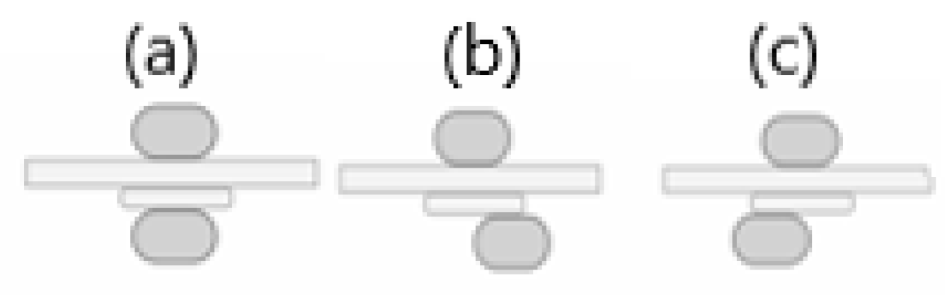
| Hole | The specimen with a hole placed over the center of the transmitter |
| No Hole | The specimen with no hole placed over the center of the transmitter |
| Hole Filled | The specimen with a hole filled with silicone placed over the center of the transmitter |
| Hole Right | The specimen with a hole placed so that the center is to the right of the transmitter |
| No Hole Right | The specimen with no hole placed so that the center is to the right of the transmitter |
| Hole Filled Right | The specimen with a hole filled with silicone placed so that the center is to the right of the transmitter |
| Hole Left | The specimen with a hole placed so that the center is to the left of the transmitter |
| No Hole Left | The specimen with no hole placed so that the center is to the left of the transmitter |
| Hole Filled Left | The specimen with a hole filled with silicone placed so that the center is to the left of the transmitter |
Publisher’s Note: MDPI stays neutral with regard to jurisdictional claims in published maps and institutional affiliations. |
© 2022 by the authors. Licensee MDPI, Basel, Switzerland. This article is an open access article distributed under the terms and conditions of the Creative Commons Attribution (CC BY) license (https://creativecommons.org/licenses/by/4.0/).
Share and Cite
Jarreau, B.; Yoshida, S.; Laprime, E. Deep Machine Learning for Acoustic Inspection of Metallic Medium. Vibration 2022, 5, 530-556. https://doi.org/10.3390/vibration5030030
Jarreau B, Yoshida S, Laprime E. Deep Machine Learning for Acoustic Inspection of Metallic Medium. Vibration. 2022; 5(3):530-556. https://doi.org/10.3390/vibration5030030
Chicago/Turabian StyleJarreau, Brittney, Sanichiro Yoshida, and Emily Laprime. 2022. "Deep Machine Learning for Acoustic Inspection of Metallic Medium" Vibration 5, no. 3: 530-556. https://doi.org/10.3390/vibration5030030
APA StyleJarreau, B., Yoshida, S., & Laprime, E. (2022). Deep Machine Learning for Acoustic Inspection of Metallic Medium. Vibration, 5(3), 530-556. https://doi.org/10.3390/vibration5030030