Optimal Placement and Active Control Methods for Integrating Smart Material in Dynamic Suppression Structures

Abstract

To simulate a lightweight structure with integrated actuators and sensors, two-dimensional finite elements are utilized. The study looks at the optimal location and active vibration control for a piezoelectric smart flexible structure. Intelligent applications are commonly used in engineering applications. In computational mechanics, selecting the ideal position for actuators to suppress oscillations is crucial. The structure oscillates due to dynamic disturbance, and active control is used to try to reduce the oscillation. Utilizing an LQR and H_infinity controller, optimization is carried out to determine the best controller weights, which will dampen the oscillation. Challenging issues arise in the design of control techniques for piezoelectric smart structures. Piezoelectric materials have been investigated for use in distributed parameter systems (for example airplane wings, intelligent bridges, etc.) to provide active control efficiently and affordably. Still, no full suppression of the oscillation with this approach has been achieved so far. The controller’s order is then decreased using optimization techniques. Piezoelectric actuators are positioned optimally according to an enhanced optimization method. The outcomes demonstrate that the actuator optimization strategies used in the piezoelectric smart single flexible manipulator system have increased observability in addition to good vibration suppression results.

1. Introduction

The terms “smart”, “intelligent”, and “adaptive” were first used to characterize the newly developing field of study that included incorporating electroactive functional materials into large constructions as in situ actuators and sensors in the middle of the 1980s [1,2,3,4,5,6,7]. In the past, electroactive materials were only employed in small- and micro-scale transducers and accurate mechatronics (electrical and mechanical) regulation systems. The common notion of intelligent, smart, and adaptable materials or constructs suggests the capability to be sharp, clever, fashionable, active, and advanced. In reality, however, real intelligence or thinking cannot be achieved by materials or structures due to the lack of artificial intelligence. Furthermore, the concept of a structure has been redefined as an adaptive or active (lifelike) multifunctional construct of an electronic system with essential abilities for diagnosis, self-sensing, and control [1,2,3,4]. Modeling and control are common approaches in manufacturing systems [8,9].

Control theory is a common approach for the optimization of materials in the engineering field [10,11]. Additionally, robust control methods have been applied in smart materials in the past [12]. Herein, we make use of piezoelectric components. When quartz crystals were exposed to mechanical forces in 1880, the Curie brothers (Pierre and Jacques) detected the creation of electric fields on the crystals (the Greek word piezo means “press”) [1,2,3,4]. In general, piezoelectricity connects the electric and elastic fields by electromechanical means. When a piezoelectric material reacts to mechanical strain or stress by generating electric charges or voltages, this is known as the explicit piezoelectric effect. When electric charges or fields are given to a material, the resulting mechanical stresses or strains have the opposite of the piezoelectric effect [5,6,7,13]. For sensor applications, the direct effect often serves as the foundation, while the opposite effect is used for precise manipulation and actuation in control uses. It is actuated. Based on designs and configurations, or whether mechanical expansions or reductions are used with or without lever systems, the actuation stroke can range from nano- to micro- to millimeter scales. It should be noted that piezoelectricity is a first-order action at low electric fields that results in strain proportional to the electric field and displacement direction, dependent on the sign of the electric field [4,5,6,7,13]. Many researchers are interested in piezoelectric materials and their applications in mechanical structures [13,14,15,16,17,18,19,20,21]. In our paper, we investigate the optimal placement of piezoelectric material in mechanical structures and their application in vibration suppression using Linear–quadratic regulator (LQR) control and Hinfinity (H_∞) control methods. For example, the appropriate position could be selected by modeling the equipment or simulating the process [22]. Many important researchers have dealt with the problem of control in smart construction [23,24,25]. In this paper, the problem of topological optimization of structures is presented [25], while in our thesis the modeling of the vector and the complete suppression of oscillations are presented in detail.

Designing control methods for piezoelectric smart structures presents difficult problems. To offer active control effectively and economically, piezoelectric materials have been researched for application in distributed parameter systems. Distributed sensors and actuators made of piezoelectric materials with adaptive qualities can be utilized to actively regulate dynamic systems. In this essay, we discuss the key considerations that structural control engineers must make while developing trustworthy control methods for evaluating resilience, optimum placement, and structural modeling under uncertainty.

Suppression of vibrations under dynamic and uncertain loading is a very serious engineering problem. Vibrations are important in engineering systems, as they are connected with the fatigue of the materials, which leads to catastrophic failures and the end of life for parts. The application to simpler models allows the application of advanced control techniques since the controller presented is of order 36. All simulations have been completed in Matlab with advanced programming techniques.

In this work, we achieve full suppression of oscillations with two control strategies, the Hinfinity control and the LQR. First, a smart structure is modeled with integrated piezoelectric elements that act as both sensors and actuators. Afterward, an optimal placement is made in their place. Modeling uncertainties as well as measurement noise are taken into account, and then advanced control techniques are applied. The results are presented both in the time domain and in the frequency domain. The following are the benefits of this work:

-

Modeling of intelligent constructs execution of control in oscillation suppression.

-

Uncertainties in dynamic loading.

-

Measurement noise.

-

Appropriate selection of weights for complete suppression of oscillations.

-

Using various choice places to stifle oscillations.

-

Results in the frequency domain as well as the time-space domain.

-

Introduction of the uncertainties in the construction’s mathematical model.

2. Modeling

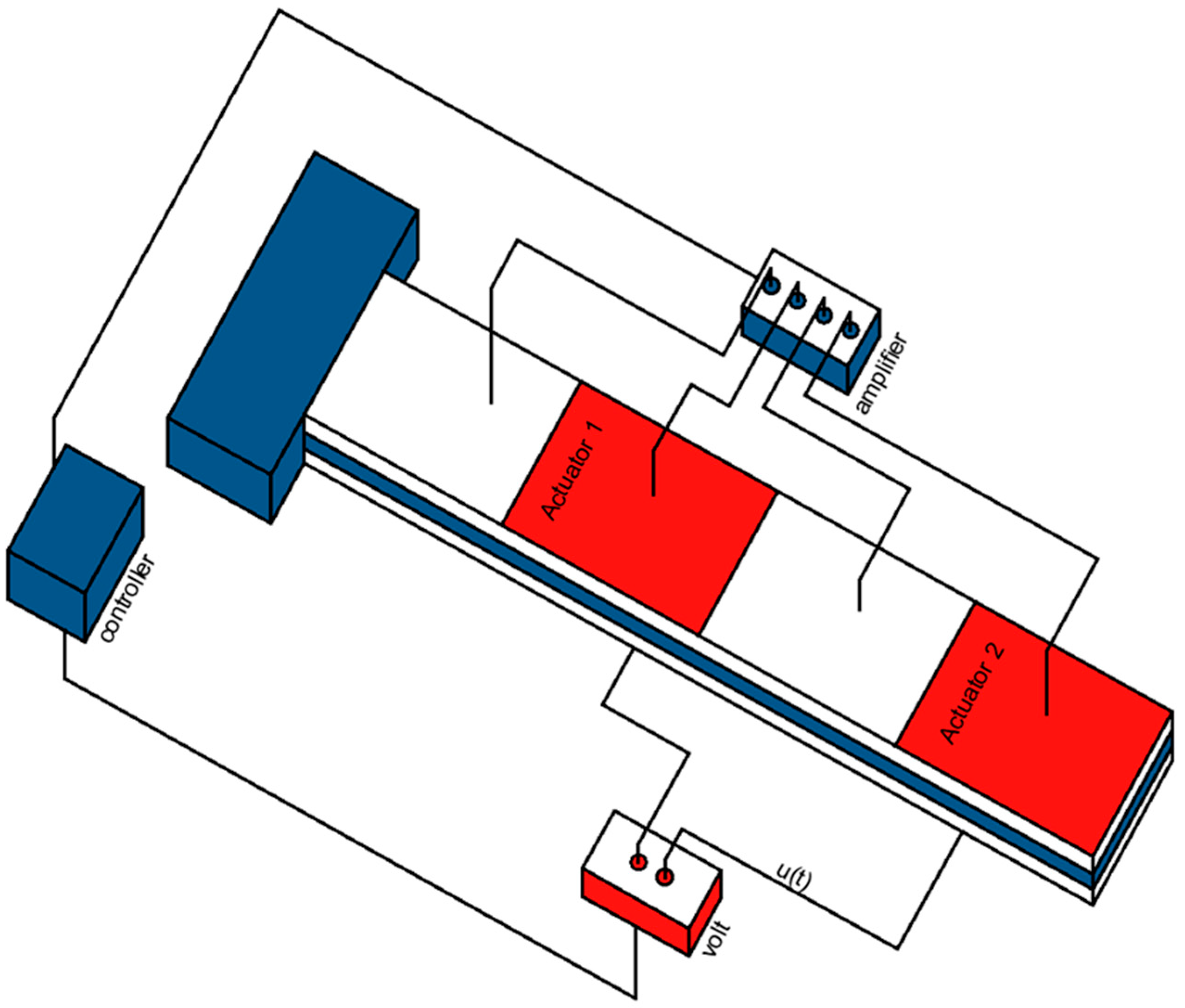
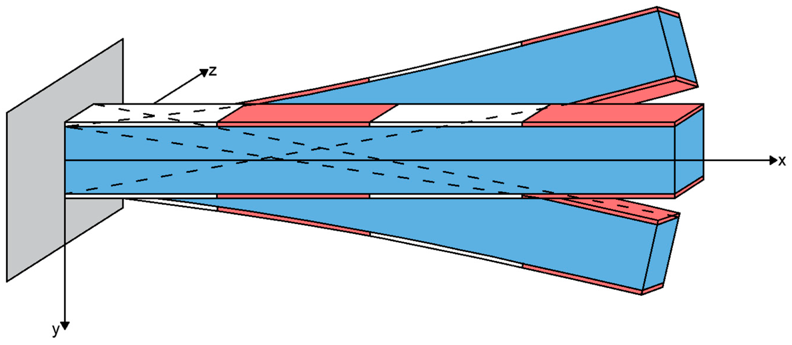
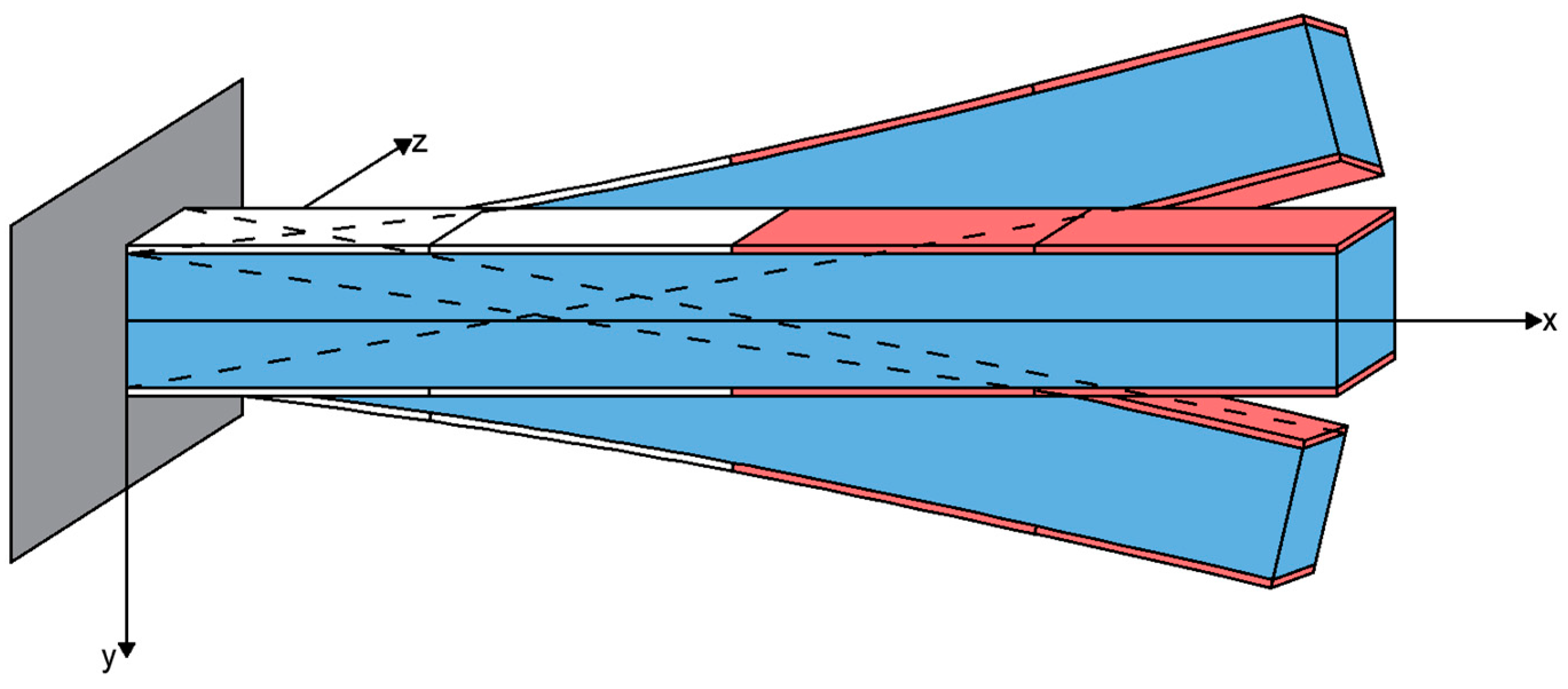
This work deals with the reduction of oscillations using piezoelectric and advanced control techniques. Two cases of piezoelectric placement are taken. In Figure 1 (the first case), the actuators have been placed alternately, i.e., in positions 2 and 4. In Figure 2 (the second case) the actuators have been placed at the end of the beam and concentrated in positions 3 and 4, i.e., in the second half. The sensor output will be used for control actions [26]. The literature compared data-driven choices vs. simulation-based solutions [27,28,29].

Figure 1. (The first case), the actuators have been placed alternately, i.e., in positions 2 and 4.

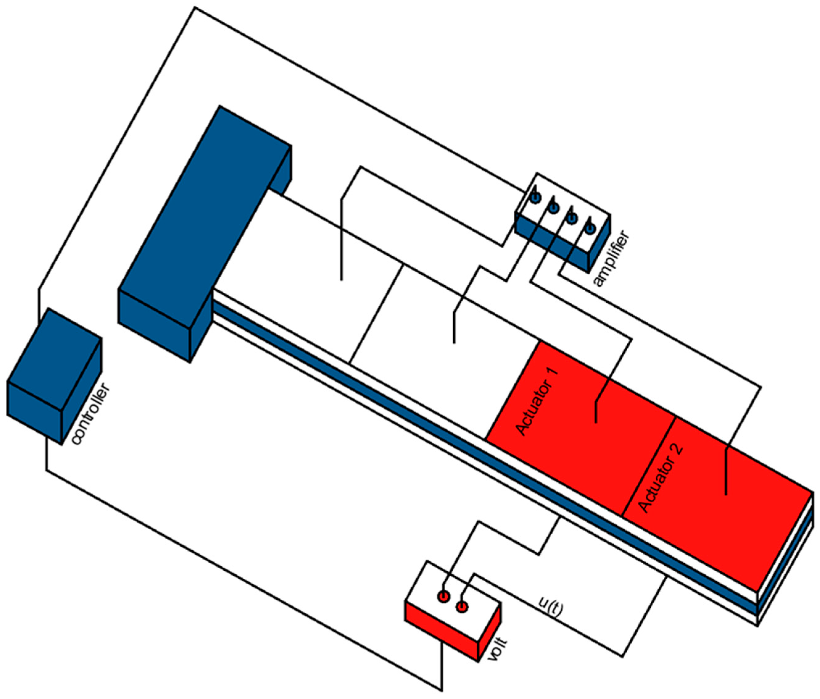
Figure 2. (The second case) the actuators have been placed at the end of the beam and concentrated in positions 3 and 4.

The specific beam model simulated with two-dimensional finite elements has been chosen because it can be modeled and advanced control techniques can be applied to it that take into account modeling essentials such as unknown disturbances and uncertainties of modeling. This particular model is a cantilever beam that can simulate an airplane wing or a bridge. With assumptions, the unknown disturbances may be the great force of the wind or the earthquake. In this work, the force of the wind is taken into account. In the literature given, relevant models have been used, but the results presented herein are much better, compared to the other reports, because the oscillations are completely suppressed. Suppression of vibrations under dynamic and uncertain loading is a very serious engineering problem. The application to simpler models allows the application of advanced control techniques since the controller presented is of order 36. All simulations have been completed in Matlab with advanced programming techniques.

The dynamical description of the system is given by:

$$\mathrm{M}\ddot{q}\left(t\right)+\mathrm{D}\dot{q}\left(t\right)+\mathrm{K}q\left(\mathrm{t}\right)={\mathrm{f}}_{\mathrm{m}}\left(\mathrm{t}\right)+{\mathrm{f}}_{\mathrm{e}}\left(\mathrm{t}\right)$$

(1)

where f_m is the global external loading mechanical vector, K is the global stiffness matrix, M is the global mass matrix, and D is the viscous damping matrix. It is difficult to specify how structural damping is determined because there are so many variables involved. To keep things simple, the structural damping matrix D can be analyzed as either linearly combined mass or stiffness (Rayleigh damping), which is D = αM + βK, or as mass proportional. Here α and β are calculated in terms of the first and second normal mode of vibration, α and β are 0.0005, and f_e is the global control force vector resulting from electromechanical coupling effects. Rotations w_i and transversal deflections ψ_i make up the unrelated variable q(t), or

$$q\left(t\right)=\left[\begin{array}{c}{\mathrm{w}}_1\\ {\mathsf{\psi }}_1\\ ⋮\\ {\mathrm{w}}_{\mathrm{n}}\\ {\mathsf{\psi }}_{\mathrm{n}}\end{array}\right]$$

(2)

where n represents how many finite elements were employed in the analysis.

Let us (as is customary) translate to a state-space control interpretation.

$$\begin{gathered} X(t)=\left[\begin{array}{c}q\left(t\right)\\ \dot{q}\left(t\right)\end{array}\right] \\ \dot{x}\left(t\right)=\left[\begin{array}{c}{0}_{2\mathrm{n}\times \mathrm{n}}\\ {\mathrm{M}}^{-1}({\mathrm{f}}_{\mathrm{m}}\left(\mathrm{t}\right)+{\mathrm{f}}_{\mathrm{e}}\left(\mathrm{t}\right)\end{array}\right]+\left[\begin{array}{c}\dot{q}\left(t\right)\\ -{\mathrm{M}}^{-1}\mathrm{D}\dot{q}\left(t\right)-{\mathrm{M}}^{-1}\mathrm{K}q\left(t\right)\end{array}\right] \\ =\left[\begin{array}{c}{0}_{2\mathrm{n}\times \mathrm{n}}\\ {\mathrm{M}}^{-1}\left({\mathrm{f}}_{\mathrm{m}}+{\mathrm{f}}_{\mathrm{e}}\right)\left(\mathrm{t}\right)\end{array}\right]+\left[\begin{array}{cc}\begin{array}{c}{0}_{2\mathrm{n}\times 2\mathrm{n}}\\ -{\mathrm{M}}^{-1}\mathrm{K}\end{array}& \begin{array}{c}{\mathrm{I}}_{2\mathrm{n}\times 2\mathrm{n}}\\ -{\mathrm{M}}^{-1}\mathrm{D}\end{array}\end{array}\right]\left[\begin{array}{c}q\left(t\right)\\ \dot{q}\left(t\right)\end{array}\right] \\ =\left[\begin{array}{c}{0}_{2\mathrm{n}\times \mathrm{n}}\\ {\mathrm{M}}^{-1}{\mathrm{f}}_{\mathrm{m}}\left(\mathrm{t}\right)\end{array}\right]+\left[\begin{array}{c}{0}_{2\mathrm{n}\times \mathrm{n}}\\ {\mathrm{M}}^{-1}{\mathrm{f}}_{\mathrm{e}}\left(\mathrm{t}\right)\end{array}\right]+\left[\begin{array}{cc}\begin{array}{c}{0}_{2\mathrm{n}\times 2\mathrm{n}}\\ -{\mathrm{M}}^{-1}\mathrm{K}\end{array}& \begin{array}{c}{\mathrm{I}}_{2\mathrm{n}\times 2\mathrm{n}}\\ -{\mathrm{M}}^{-1}\mathrm{D}\end{array}\end{array}\right]\left[\begin{array}{c}q\left(t\right)\\ \dot{q}\left(t\right)\end{array}\right]. \end{gathered}$$

(3)

Additionally, we define f_e(t) = F_e × u(t) as, where (of size 2n × n) is the piezoelectric force for a unit put on the appropriate actuator,

Where:

$$F_e=\left[\begin{array}{cccc}0& 0& 0& 0\\ cp& -cp& 0& 0\\ 0& 0& 0& 0\\ 0& cp& -cp& 0\\ 0& 0& 0& 0\\ 0& 0& cp& -cp\\ 0& 0& 0& 0\\ 0& 0& 0& cp\end{array}\right]$$

(4)

and u(t) denotes the voltages on the actuators. Finally, the disturbance vector is the mechanical force d(t) = f_m(t). Then,

$$\begin{gathered} \dot{x}\left(t\right)=\left[\begin{array}{cc}{0}_{2\mathrm{n}\times 2\mathrm{n}}& {\mathrm{I}}_{2\mathrm{n}\times 2\mathrm{n}}\\ -{\mathrm{M}}^{-1}\mathrm{K}& -{\mathrm{M}}^{-1}D\end{array}\right]x\left(t\right)+\left[\begin{array}{c}{0}_{2\mathrm{n}\times \mathrm{n}}\\ {\mathrm{M}}^{-1}{\mathrm{F}}_{\mathrm{e}}^{\ast }\end{array}\right]u\left(t\right)+\left[\begin{array}{c}{0}_{2\mathrm{n}\times 2\mathrm{n}}\\ {\mathrm{M}}^{-1}\end{array}\right]d\left(t\right) \\ =\mathsf{A}x\left(t\right)+\mathsf{{\rm B}}u\left(t\right)+\mathrm{G}d\left(t\right) \\ =\mathrm{A}x\left(t\right)+\left[\mathrm{B} \mathrm{G}\right] \left[\begin{array}{c}u\left(t\right)\\ d\left(t\right)\end{array}\right] \\ =\mathrm{A}x\left(t\right)+ \mathrm{B} ˜\tilde{u}\left(t\right). \end{gathered}$$

(5)

With the output equation (displacements are just measured), we can improve this.

y(t) = [x₁(t) x₃(t) … x_n−1(t)]T = Cx(t).

(6)

The parameters of our system are in Table 1 and Figure 3 and Figure 4. To measure the state of the system, respective piezoelectric sensors are used. The voltage of the sensor outputs is proportional to the nodal movements of the corresponding elements. Therefore, the output of the system is given by Equation (6). In this example, four finite elements are used, so the measurements are possible. In addition, the table C is as follows:

C = [1 0 0…0; −1 0 1 0…0; 0 0 −1 0 1…0; 0 0 0 0 −1 0 1…0].

Table 1. Factors of the smart beam.

Parameters	Values
L, for Beam length	1.00 m
W, for Beam width	0.08 m
h, for Beam thickness	0.02 m
ρ, for Beam density	1600 kg/m3
E, for Young’s modulus of the Beam	1.5 × 1011 N/m2
bs, ba, for Pzt thickness	0.002 m
d31 the Piezoelectric constant	280 × 10−12 m/V

Figure 3. The actuators have been placed alternately, i.e., in positions 2 and 4 (the red color indicates these positions, the blue color is the beam without piezoelectric patches and the white color is the remaining two positions 1 and 3, without actuator).

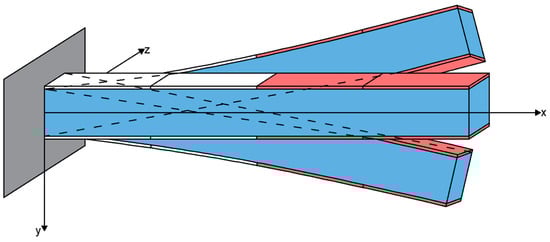
Figure 4. The actuators have been placed at the end of the beam and concentrated in positions 3 and 4 (the red color indicates these positions, the blue color is the beam without piezoelectric patches and the white color is the remaining two positions 1 and 2, without actuator).

3. Controller Synthesis

The challenge is to model the uncertainty in both the external disturbance and the simulation model, while there is the optimal placement of the actuators. The benefits are that infinite control considers uncertainties, complete suppression of oscillations, and the results in the state space and the frequency domain. All simulations have been conducted with advanced design techniques.

The aforementioned give ways for comparing and assessing controller performance as well as analytical difficulties. However, a controller that achieves a certain behavior in terms of the constructed singular value may be roughly synthesized. In this process identified as the (D, G-K) iteration [18,30], the challenge of locating an optimal controller Κ(s) such that μ(F_u(F(jω), Κs(jω)) ≤ β, ∀ω is transmuted into the difficulty of discovering transfer function matrices D(ω) ∈ H and G(ω) ∈ H, such that,

$$\underset{\mathsf{\omega }}{\sup }\overline{\mathsf{\sigma }}\left[\left(\frac{D\left(\omega \right)({\mathrm{F}}_{\mathrm{u}}\left(\mathrm{F}\left(\mathrm{j}\mathsf{\omega }\right),\mathsf{{\rm K}}\left(\mathrm{j}\mathsf{\omega }\right)\right)D^{-1}\left(\omega \right)}{\mathsf{\gamma }}-\mathrm{jG}\left(\mathsf{\omega }\right)\right){\left(\mathrm{I}+{\mathrm{G}}^2\left(\omega \right)\right)}^{-\frac{1}{2}}\right]\le 1,\begin{array}{c}\forall \mathrm{\omega }\end{array}.$$

(7)

Unfortunately, this approach does not ensure even discovering local maxima. Nevertheless, for complicated perturbations a technique known as the D-K iteration is accessible (also executed in Matlab) [24,31,32]. It relates to the H_∞ synthesis and frequently generates good outcomes. The initial point is the maximum value of μ in terms of the scaled singular value, where:

$$\mathsf{\mu }\left(\mathrm{N}\right)\le \underset{\mathrm{D}\in \mathrm{D}}{\min }\overline{\mathsf{\sigma }}\left(D\mathrm{N}{D}^{-1}\right).$$

(8)

The concept is to discover the controller that minimalizes the peak over frequency of its upper bound [17], namely,

$$\underset{\mathrm{K}}{\min }\left(\underset{\mathrm{D}\in \mathrm{D}}{\min }\Vert D\mathrm{N}\left(\mathrm{K}\right)D^{-1}{\Vert }_{\infty }\right),$$

(9)

by changing between minimalizing $\Vert DN\left(K\right)D^{-1}{\Vert }_{\infty }$ with regard to either K or D (while keeping the other attached) [33,34,35].

• K-step. Create a controller for the scaled issue. $\underset{K}{\min }\Vert DN\left(K\right)D^{-1}{\Vert }_{\infty }$ with fixed D(s).
• D-step. Find D(jω) to minimalize at each frequency $\overline{\sigma }\left(DN{D}^{-1}\left(\mathrm{j}\omega \right)\right)$ with fixed N.
• Fit the degree of each factor of D(jω) to a stable and the lowest phase transfer function D(s) and move to Step 1.

4. Results

4.1. Results in Simulation and Analysis of the Smart Structural Control

The presented problem takes as input the disturbance and measurement noise and gives as output the controller voltages and displacement measurements. The equations and structural diagrams presented analyze the equations used to model the specific problem of the beam and are used in programming using Matlab.

Our goal is to identify the best transfer function N of the system.

Deriving the input-output relations for the first model is helpful for this purpose.

$$\left[\begin{array}{c}u\\ \mathrm{e}\end{array}\right]=\mathrm{F}\left(\mathrm{s}\right)\left[\begin{array}{c}d\\ \mathrm{n}\end{array}\right]\Rightarrow z=\mathrm{F}\left(\mathrm{s}\right)\mathrm{w}.$$

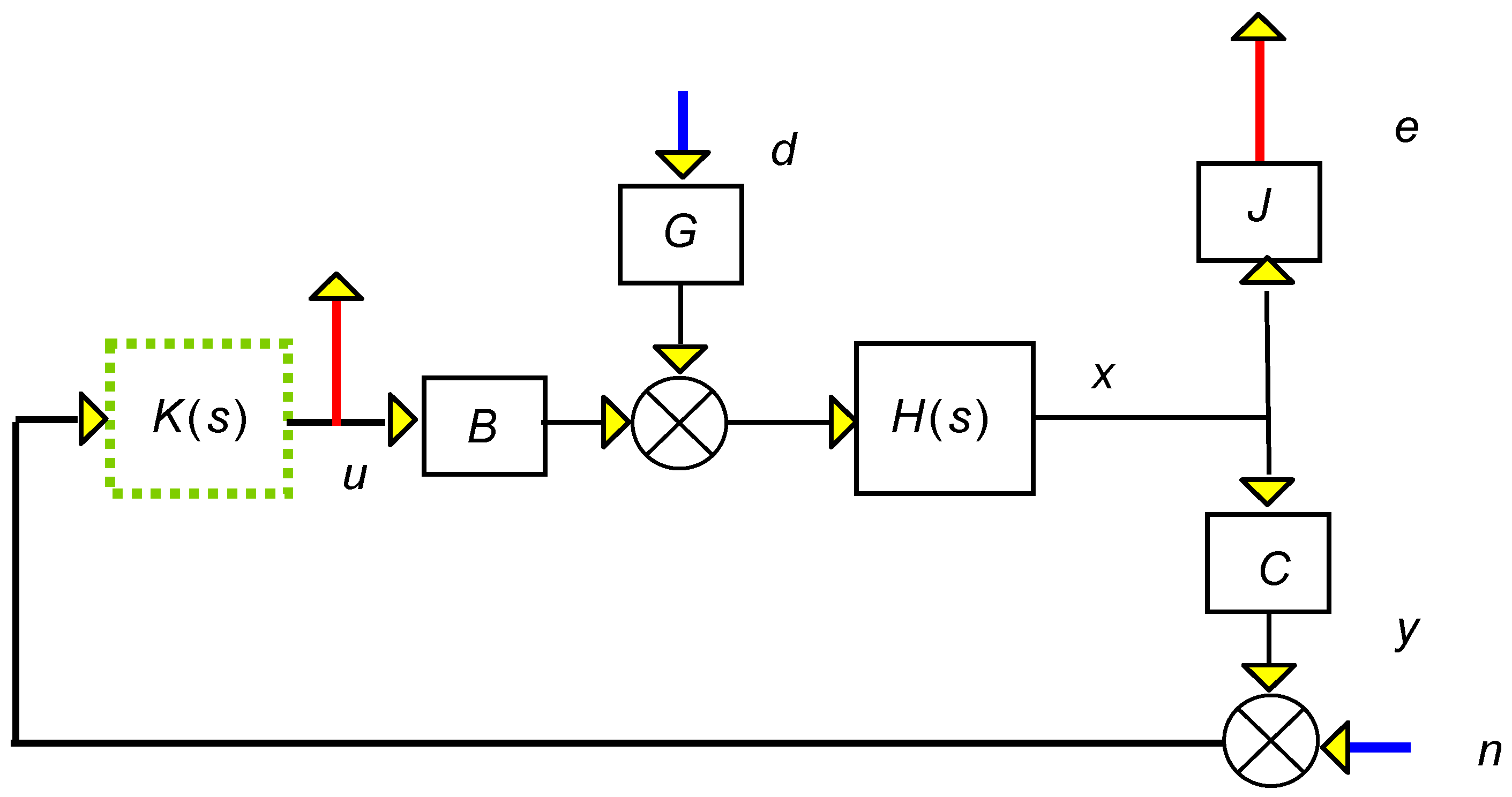
u and e are the outputs (control, error), and d, n are the inputs (disturbance, noise) as illustrated in Figure 5.

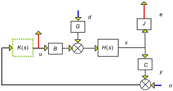
Figure 5. Beam with a controller, disturbance input, error, and noise output.

Where the beam is explained by the state space domain

$$\dot{x}\left(t\right)= \mathrm{A}x(t)+[\mathrm{B} \mathrm{G}] \left[\begin{array}{c}u\left(t\right)\\ d\left(t\right)\end{array}\right].$$

In the frequency domain, our system is as follows:

H(s) = (sI − A)⁻¹,

(10)

and J is utilized to select those states that we are concerned with controlling (which may be altered from y). In the majority of the investigations, J will be:

$$\mathrm{J}=\left[\begin{array}{cccccccccccccccc}1& 0& 0& 0& 0& 0& 0& 0& 0& 0& 0& 0& 0& 0& 0& 0\\ 0& 0& 1& 0& 0& 0& 0& 0& 0& 0& 0& 0& 0& 0& 0& 0\\ 0& 0& 0& 0& 1& 0& 0& 0& 0& 0& 0& 0& 0& 0& 0& 0\\ 0& 0& 0& 0& 0& 0& 1& 0& 0& 0& 0& 0& 0& 0& 0& 0\end{array}\right]$$

(11)

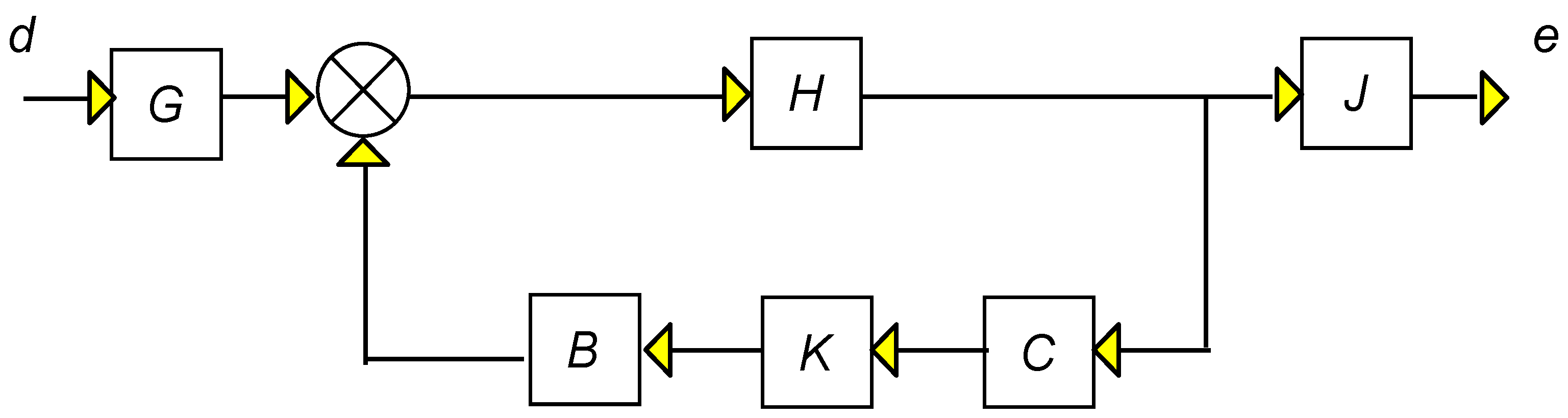
We start by redrawing Figure 5 successively.

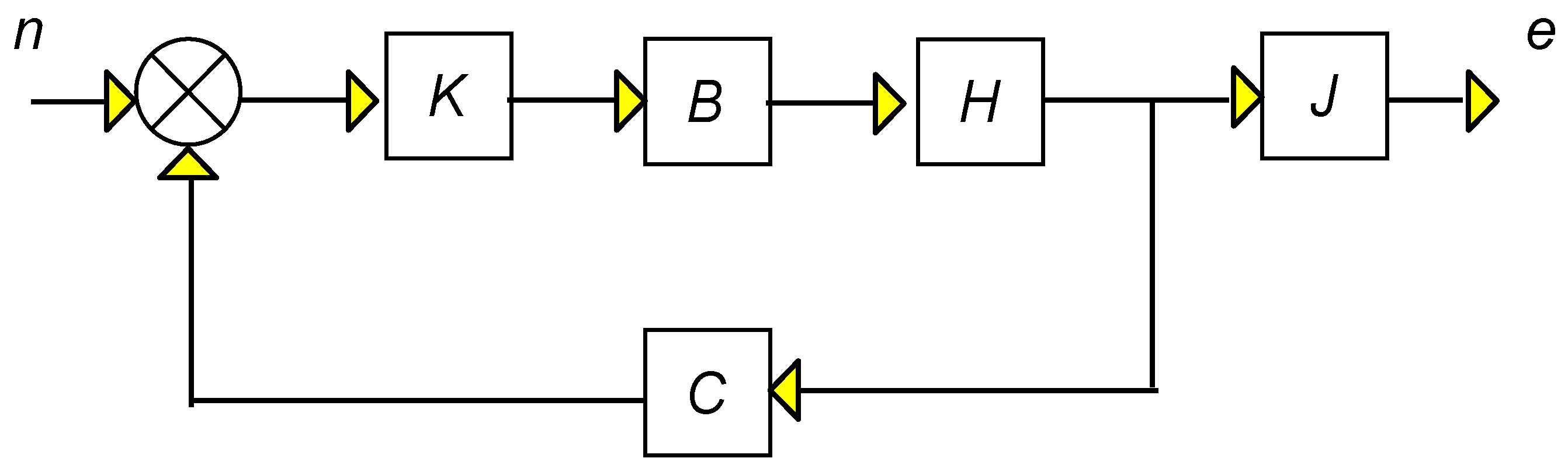
From Figure 6 it is easily seen that T_de (transfer function disturbance to error) is

T_de = J × (I − HBKC)⁻¹H × G.

(12)

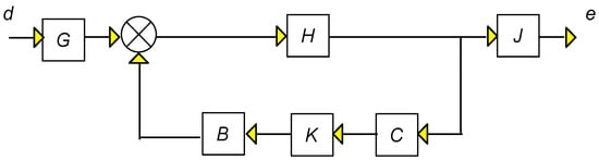
Figure 6. Block diagram disturbance, errors.

From Figure 7 it is seen that T_ne (transfer function noise to error) is

T_ne = J × (I − HBKC)⁻¹HBK.

(13)

Figure 7. Block diagram noise, and errors.

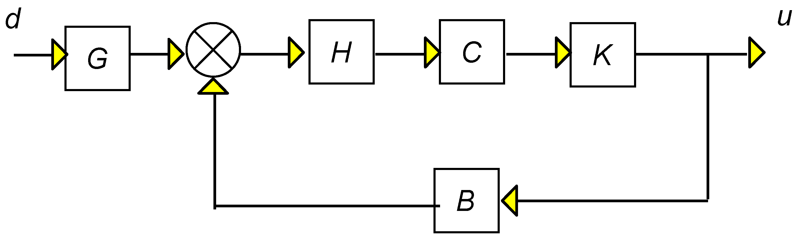
From Figure 8 it is seen that T_du (transfer function disturbance to control) is

T_du = (I − KCHB)⁻¹KCH × G.

(14)

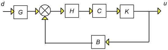
Figure 8. Block diagram disturbance, control voltages.

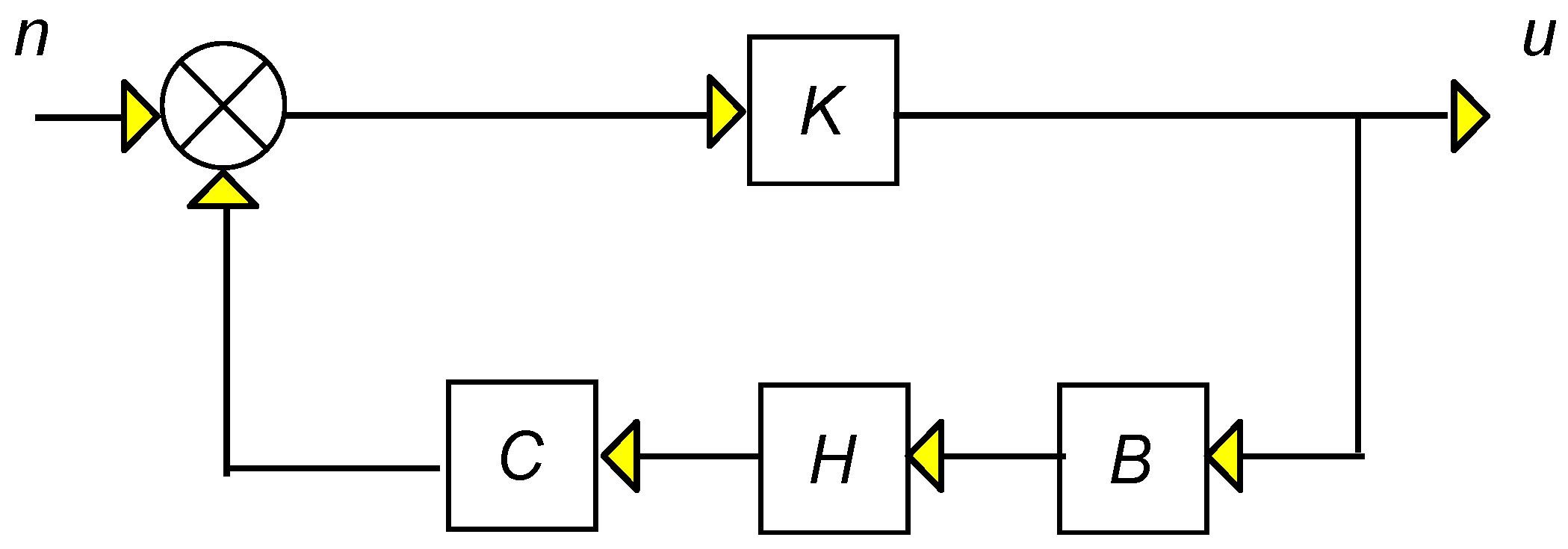
From Figure 9 it is seen that T_nu (transfer function noise to control) is

T_nu = (I − KCHB)⁻¹K.

(15)

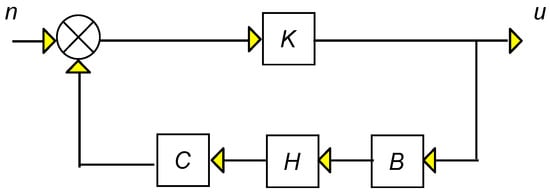
Figure 9. Block diagram noise, and control voltages.

Combining we find,

e = J × (I − HBKC)⁻¹H × Gd + J × (I − HBKC)⁻¹HBKn

(16)

and

u = (I − KCHB)⁻¹KCH × Gd + (I − KCHB)⁻¹Kn

(17)

or,

$$\left[\begin{array}{c}u\\ \mathrm{e}\end{array}\right]=\left[\begin{array}{cc}{\left(\mathrm{I}-\mathrm{KCHB}\right)}^{-1}\mathrm{KCHG}& {\left(\mathrm{I}-\mathrm{KCHB}\right)}^{-1}\mathrm{K}\\ \mathrm{J}{\left(\mathrm{I}-\mathrm{HBKC}\right)}^{-1}\mathrm{HG}& \mathrm{J}{\left(\mathrm{I}-\mathrm{HBKC}\right)}^{-1}\mathrm{HBK}\end{array}\right]\left[\begin{array}{c}d\\ \mathrm{n}\end{array}\right]$$

(18)

and

$$\left[\begin{array}{c}u\\ \mathrm{e}\end{array}\right]=\left[\begin{array}{cc}{\mathrm{F}}_{\mathrm{du}}& {\mathrm{F}}_{\mathrm{nu}}\\ {\mathrm{F}}_{\mathrm{de}}& {\mathrm{F}}_{\mathrm{ne}}\end{array}\right]\left[\begin{array}{c}\mathrm{d}\\ \mathrm{n}\end{array}\right]\Rightarrow z=\mathrm{F}\left(\mathrm{s}\right)\mathrm{w}.$$

(19)

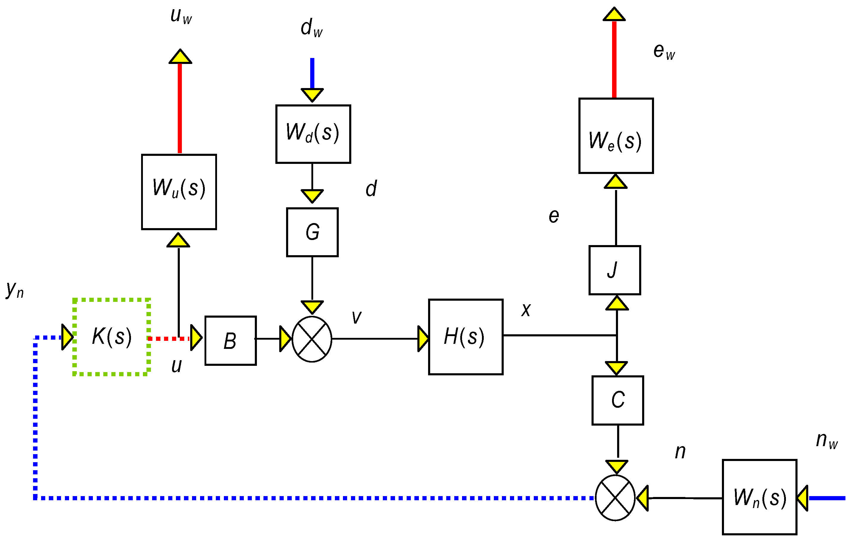
To continue, we adjust the weighting appropriately and redesign Figure 5 to suit our specific problem:

Subsequently, we create a new representation of Figure 10 in the form of a two-port diagram, similar to the layout shown in Figure 6 for comparison:

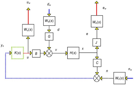
Figure 10. Block diagram with weights considered for the beam scenario.

In Figure 11, x and v are auxiliary signals.

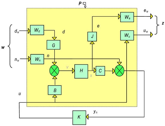
Figure 11. Two-port diagram for the beam problem.

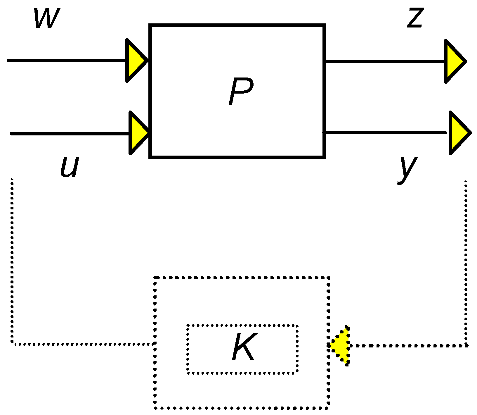
We are looking for:

Q_zw(s) = P_zw(s) + P_zu(s)K(s) (I − P_yu(s)K(s))⁻¹P_yw(s)

(20)

such that

z = Q_zww = F(P, K)w.

(21)

We want to locate P(s). The required transfer performers are:

e_w = W_eJx= W_eJHv = W_eJH(GW_dd_w + Bu) = W_eJHGW_dd_w + W_eJHBu,

(22)

u_w = W_uu,

(23)

and

y_n = Cx + W_nn_w = CHv + W_nn_w = CH(GW_dd_w + Bu) + W_nn_w=

CHGW_dd_w + CHBu + W_nn_w.

(24)

Combining all these gives

$$\left[\begin{array}{c}{u}_w\\ {\mathrm{e}}_{\mathrm{w}}\\ y_n\end{array}\right]=\left[\begin{array}{ccc}0& 0& {\mathrm{W}}_{\mathrm{u}}\\ {\mathrm{W}}_{\mathrm{e}}{\mathrm{JHGW}}_{\mathrm{d}}& 0& {\mathrm{W}}_{\mathrm{e}}\mathrm{JHB}\\ {\mathrm{CHGW}}_{\mathrm{d}}& {\mathrm{W}}_{\mathrm{n}}& \mathrm{CHB}\end{array}\right]\left[\begin{array}{c}{d}_w\\ {\mathrm{n}}_{\mathrm{w}}\\ u\end{array}\right],$$

(25)

or

$$\left[\begin{array}{c}z\\ y_n\end{array}\right]=\left[\begin{array}{cc}{\mathrm{P}}_{\mathrm{zw}}& {\mathrm{P}}_{\mathrm{zu}}\\ {\mathrm{P}}_{\mathrm{yw}}& {\mathrm{P}}_{\mathrm{yu}}\end{array}\right]\left[\begin{array}{c}\mathrm{w}\\ u\end{array}\right],$$

(26)

where:

$${\mathrm{P}}_{\mathrm{zw}}=\left[\begin{array}{cc}0& 0\\ {\mathrm{W}}_{\mathrm{e}}{\mathrm{JHGW}}_{\mathrm{d}}& 0\end{array}\right],\begin{array}{c} \end{array}{\mathrm{P}}_{\mathrm{zu}}=\left[\begin{array}{c}{\mathrm{W}}_{\mathrm{u}}\\ {\mathrm{W}}_{\mathrm{e}}\mathrm{JHB}\end{array}\right],\begin{array}{c} \end{array}{\mathrm{P}}_{\mathrm{yw}}=\left[\begin{array}{cc}{\mathrm{CHGW}}_{\mathrm{d}}& {\mathrm{W}}_{\mathrm{n}}\end{array}\right],\begin{array}{c} \end{array}{\mathrm{P}}_{\mathrm{yu}}=\mathrm{CHB}.$$

(27)

An additional step is required, however, to acquire the Q_ij’s. We achieve this utilizing Equation (18) and noticing that:

d = W_dd_w, n = W_nn_w, e_w = W_ee, u_w = W_uu.

Hence,

$$\begin{array}{c}\left[\begin{array}{c}u\\ \mathrm{e}\end{array}\right]=\left[\begin{array}{c}{\mathrm{W}}_{\mathrm{u}}^{-1}{u}_w\\ {\mathrm{W}}_{\mathrm{e}}^{-1}{\mathrm{e}}_{\mathrm{w}}\end{array}\right]=\mathrm{F}\left(\mathrm{s}\right)\left[\begin{array}{c}d\\ \mathrm{n}\end{array}\right]=\mathrm{F}\left(\mathrm{s}\right)\left[\begin{array}{c}{\mathrm{W}}_{\mathrm{d}}{d}_w\\ {\mathrm{W}}_{\mathrm{n}}{\mathrm{n}}_{\mathrm{w}}\end{array}\right]\Rightarrow \\ \left[\begin{array}{c}{u}_w\\ {\mathrm{e}}_{\mathrm{w}}\end{array}\right]=\left[\begin{array}{cc}{\mathrm{W}}_{\mathrm{u}}& \\ & {\mathrm{W}}_{\mathrm{e}}\end{array}\right]\mathrm{F}\left(\mathrm{s}\right)\left[\begin{array}{cc}{\mathrm{W}}_{\mathrm{d}}& \\ & {\mathrm{W}}_{\mathrm{n}}\end{array}\right]\left[\begin{array}{c}{d}_w\\ {\mathrm{n}}_{\mathrm{w}}\end{array}\right]\end{array},$$

or

$$\left[\begin{array}{c}{u}_w\\ {\mathrm{e}}_{\mathrm{w}}\end{array}\right]=\left[\begin{array}{cc}{\mathrm{W}}_{\mathrm{u}}{\left(\mathrm{I}-\mathrm{KCHB}\right)}^{-1}{\mathrm{KCHGW}}_{\mathrm{d}}& {\mathrm{W}}_{\mathrm{u}}{\left(\mathrm{I}-\mathrm{KCHB}\right)}^{-1}{\mathrm{KW}}_{\mathrm{n}}\\ {\mathrm{W}}_{\mathrm{e}}\mathrm{J}{\left(\mathrm{I}-\mathrm{HBKC}\right)}^{-1}{\mathrm{HGW}}_{\mathrm{d}}& {\mathrm{W}}_{\mathrm{e}}\mathrm{J}{\left(\mathrm{I}-\mathrm{HBKC}\right)}^{-1}{\mathrm{HBKW}}_{\mathrm{n}}\end{array}\right]\left[\begin{array}{c}{d}_w\\ {\mathrm{n}}_{\mathrm{w}}\end{array}\right].$$

(28)

Therefore, the matrices in

$$z={ \mathrm{Q}}_{\mathrm{zw}}\mathrm{w} \mathrm{or} \left[\begin{array}{c}u\\ e\end{array}\right]=\left[\begin{array}{cc}{Q}_{11}& Q_{12}\\ Q_{21}& Q_{22}\end{array}\right]\begin{array}{c} \end{array}\left[\begin{array}{c}d\\ n\end{array}\right].$$

Regarding the formulation in the state space, we express P as a form of natural partitioning:

$$P\left(\mathrm{s}\right)=\left[\begin{array}{ccc}\mathrm{A}& {\mathrm{B}}_1& {\mathrm{B}}_2\\ {\mathrm{C}}_1& {\mathrm{D}}_{11}& {\mathrm{D}}_{12}\\ {\mathrm{C}}_2& {\mathrm{D}}_{21}& {\mathrm{D}}_{22}\end{array}\right]=\left[\begin{array}{cc}{\mathrm{P}}_{\mathrm{zw}}\left(\mathrm{s}\right)& {\mathrm{P}}_{\mathrm{zu}}\left(\mathrm{s}\right)\\ {\mathrm{P}}_{\mathrm{yw}}\left(\mathrm{s}\right)& {\mathrm{P}}_{\mathrm{yu}}\left(\mathrm{s}\right)\end{array}\right],$$

(29)

(where the condensed format has been utilized), while the related form for Κ is:

$$K\left(\mathrm{s}\right)=\left[\begin{array}{cc}{\mathrm{A}}_{\mathrm{K}}& {\mathrm{B}}_{\mathrm{K}}\\ {\mathrm{C}}_{\mathrm{K}}& {\mathrm{D}}_{\mathrm{K}}\end{array}\right].$$

Equation (29) describes the equations:

$$\begin{array}{c}\dot{x}\left(t\right)=\mathrm{A}x\left(t\right)+\left[\begin{array}{cc}{\mathrm{B}}_1& {\mathrm{B}}_2\end{array}\right]\begin{array}{c} \end{array}\left[\begin{array}{c}\mathrm{w}\left(\mathrm{t}\right)\\ u\left(t\right)\end{array}\right]\\ \left[\begin{array}{c}z\left(t\right)\\ y\left(t\right)\end{array}\right]=\left[\begin{array}{c}{\mathrm{C}}_1\\ {\mathrm{C}}_2\end{array}\right]x\left(t\right)+\left[\begin{array}{cc}{\mathrm{D}}_{11}& {\mathrm{D}}_{12}\\ {\mathrm{D}}_{21}& {\mathrm{D}}_{22}\end{array}\right]\begin{array}{c} \end{array}\left[\begin{array}{c}\mathrm{w}\left(\mathrm{t}\right)\\ u\left(t\right)\end{array}\right]\end{array}$$

and

$$\dot{x}{}_{\mathrm{K}}\left(t\right)={\mathrm{A}}_{\mathrm{K}}{x}_{\mathrm{K}}\left(t\right)+{\mathrm{B}}_{\mathrm{K}}y\left(t\right)$$

u(t) = C_Kx_K(t) + D_Ky(t).

To locate the matrices in question, we solve the feedback loop and apply the related equations (Figure 12):

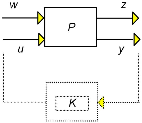
Figure 12. Open loop structure.

To obtain the arrangement in state space form, we incorporate the outputs, inputs, states, and input/output to the controller:

$$\begin{gathered} {\dot{x}}_F=\mathrm{A}{x}_F+\left(\mathrm{G}d+\mathrm{B}u\right), x={\mathrm{Ix}}_{\mathrm{F}} \\ {\dot{x}}_u={\mathrm{A}}_{\mathrm{u}}{x}_u+{\mathrm{B}}_{\mathrm{u}}u, u_w={\mathrm{C}}_{\mathrm{u}}{x}_u+{\mathrm{D}}_{\mathrm{u}}u \\ {\dot{x}}_e={\mathrm{A}}_{\mathrm{e}}{x}_e+{\mathrm{B}}_{\mathrm{e}}\mathrm{J}x,\begin{array}{c} \end{array}{\mathrm{e}}_{\mathrm{w}}={\mathrm{C}}_{\mathrm{e}}{x}_e+{\mathrm{D}}_{\mathrm{e}}\mathrm{J}x \\ {\dot{x}}_{nw}={\mathrm{A}}_{\mathrm{nw}}{x}_{nw}+{\mathrm{B}}_{\mathrm{nw}}{\mathrm{n}}_{\mathrm{w}}, \mathrm{n}={\mathrm{C}}_{\mathrm{nw}}{x}_{nw}+{\mathrm{D}}_{\mathrm{nw}}{\mathrm{n}}_{\mathrm{w}} \\ {\dot{x}}_{dw}={\mathrm{A}}_{\mathrm{dw}}{x}_{dw}+{\mathrm{B}}_{\mathrm{dw}}{d}_w,d={\mathrm{C}}_{\mathrm{dw}}{x}_{dw}+{\mathrm{D}}_{\mathrm{dw}}{d}_w \\ y= \mathrm{C}x+ \mathrm{n}. \end{gathered}$$

(30)

Let

$$x=\left[\begin{array}{c}{x}_F\\ x_u\\ x_e\\ x_{nw}\\ x_{dw}\end{array}\right],\begin{array}{c} \end{array}y=y ,\begin{array}{c} \end{array}\mathrm{w}=\left[\begin{array}{c}{\mathrm{d}}_{\mathrm{w}}\\ {\mathrm{n}}_{\mathrm{w}}\end{array}\right],\begin{array}{c} \end{array}z=\left[\begin{array}{c}{u}_w\\ {\mathrm{e}}_{\mathrm{w}}\end{array}\right],\begin{array}{c} \end{array}u=u.$$

Replacing the internal signals d, n, e και x from 30 yields

$$\left[\begin{array}{c}{\dot{x}}_F\\ {\dot{x}}_u\\ {\dot{x}}_e\\ {\dot{x}}_{nw}\\ {\dot{x}}_{dw}\end{array}\right]=\left[\begin{array}{ccccc}A& 0& 0& 0& {GC}_{dw}\\ 0& A_u& 0& 0& 0\\ B_{e}J& 0& A_e& 0& 0\\ 0& 0& 0& A_{nw}& 0\\ 0& 0& 0& 0& A_{dw}\end{array}\right]\left[\begin{array}{c}{x}_F\\ x_u\\ x_e\\ x_{nw}\\ x_{dw}\end{array}\right]+\left[\begin{array}{cc}{GD}_{dw}& 0\\ 0& 0\\ 0& 0\\ 0& B_{nw}\\ B_{dw}& 0\end{array}\right]\left[\begin{array}{c}{d}_w\\ n_w\end{array}\right]+\left[\begin{array}{c}\mathrm{B}\\ B_u\\ 0\\ 0\\ 0\end{array}\right]u,$$

$$\left[\begin{array}{c}{u}_w\\ {\mathrm{e}}_{\mathrm{w}}\end{array}\right]=\left[\begin{array}{ccccc}0& {\mathrm{C}}_{\mathrm{u}}& 0& 0& 0\\ {\mathrm{D}}_{\mathrm{e}}\mathrm{J}& 0& {\mathrm{C}}_{\mathrm{e}}& 0& 0\end{array}\right]\left[\begin{array}{c}{x}_F\\ x_u\\ x_e\\ x_{nw}\\ x_{dw}\end{array}\right]+0\left[\begin{array}{c}{d}_w\\ {\mathrm{n}}_{\mathrm{w}}\end{array}\right]+\left[\begin{array}{c}{\mathrm{D}}_{\mathrm{u}}\\ 0\end{array}\right]u,$$

and

$$y=\left[\begin{array}{ccccc}\mathrm{C}& 0& 0& {\mathrm{C}}_{\mathrm{nw}}& 0\end{array}\right]\begin{array}{c} \end{array}\left[\begin{array}{c}{x}_F\\ x_u\\ x_e\\ x_{nw}\\ x_{dw}\end{array}\right]+\left[\begin{array}{cc}0& {\mathrm{D}}_{\mathrm{nw}}\end{array}\right]\begin{array}{c} \end{array}\left[\begin{array}{c}{d}_w\\ {\mathrm{n}}_{\mathrm{w}}\end{array}\right]+0u.$$

Therefore, the matrices are:

$${\mathrm{A}}_1=\left[\begin{array}{ccccc}\mathrm{A}& 0& 0& 0& {\mathrm{GC}}_{\mathrm{dw}}\\ 0& {\mathrm{A}}_{\mathrm{u}}& 0& 0& 0\\ {\mathrm{B}}_{\mathrm{e}}\mathrm{J}& 0& {\mathrm{A}}_{\mathrm{e}}& 0& 0\\ 0& 0& 0& {\mathrm{A}}_{\mathrm{nw}}& 0\\ 0& 0& 0& 0& {\mathrm{A}}_{\mathrm{dw}}\end{array}\right],\begin{array}{c} \end{array}{\mathrm{B}}_1=\left[\begin{array}{cc}\mathrm{G}{D}_{dw}& 0\\ 0& 0\\ 0& 0\\ 0& {\mathrm{B}}_{\mathrm{nw}}\\ {\mathrm{B}}_{\mathrm{dw}}& 0\end{array}\right],\begin{array}{c} \end{array}{\mathrm{B}}_2=\left[\begin{array}{c}\mathrm{B}\\ {\mathrm{B}}_{\mathrm{u}}\\ 0\\ 0\\ 0\end{array}\right],$$

$${\mathrm{C}}_1=\left[\begin{array}{ccccc}0& {\mathrm{C}}_{\mathrm{u}}& 0& 0& 0\\ D_e\mathrm{J}& 0& {\mathrm{C}}_{\mathrm{e}}& 0& 0\end{array}\right],\begin{array}{c} \end{array}{D}_{11}=0,\begin{array}{c} \end{array}{D}_{12}=\left[\begin{array}{c}{D}_u\\ 0\end{array}\right],$$

and

$${\mathrm{C}}_2=\left[\begin{array}{ccccc}\mathrm{C}& 0& 0& {\mathrm{C}}_{\mathrm{nw}}& 0\end{array}\right],\begin{array}{c} \end{array}{D}_{21}=\left[\begin{array}{cc}0& D_{nw}\end{array}\right],\begin{array}{c} \end{array}{D}_{22}=0.$$

As can be observed, the state vector in this design has a size of 16 + 4 + 4 + 4 + 8 = 36. The controller model K(s)’s size will likewise be determined by this. This sum will be decreased in the proper sequence if the particular weight matrices are constant. Next, we suppose uncertainty in the M and K matrices of the form:

K = K₀(I + k_pI_2n×2nδ_K)

M = M₀(I + m_pI_2n×2nδ_M).

(31)

Furthermore, since, D = 0.0005(K + M), a suitable form for D is

D = 0.0005[K₀(I + k_pI_2n×2nδ_K) + M₀(I + m_pI_2n×2nδ_M)]=

D₀ + 0.0005[K₀k_pI_2n×2nδ_K + M₀m_pI_2n×2nδ_M].

On the other hand, since in general,

D = αK + βM.

To keep things simple, the structural damping matrix D can be analyzed as either linearly combined mass or stiffness (Rayleigh damping), in here α and β are calculated in terms of the first and second normal mode of vibration, α and β are 0.0005. D could be stated similarly to K, M, as

D = D₀(I + d_pI_2n×2nδ_D).

In the pertinent matrices, we inject uncertainty in the form of proportion deviation. Since length can be accurately measured, this equation for uncertainty is appropriate in our situation. Uncertainty is more probable to result from terms besides the primary matrices. Here it will be assumed that:

$$║\mathsf{\Delta }{║}_{\infty } \stackrel{\mathrm{def}}{=}{\Vert \left[\begin{array}{cc}{\mathsf{{\rm I}}}_{\mathrm{n}\times \mathrm{n}}{\mathsf{\delta }}_{\mathsf{{\rm K}}}& 0_{\mathrm{n}\times \mathrm{n}}\\ 0_{\mathrm{n}\times \mathrm{n}}& {\mathsf{{\rm I}}}_{\mathrm{n}\times \mathrm{n}}{\mathsf{\delta }}_{\mathsf{{\rm M}}}\end{array}\right]\Vert }_{\infty }<1.$$

Hence, m_p and k_p are employed to scale the proportion value and the zero subscript represents nominal values.

(It is prompted that for matrix A_n×m the norm is determined via $║\mathrm{A}{║}_{\infty }=\underset{1\le \mathrm{j}\le \mathrm{m}}{\max }{\displaystyle \sum }_{\mathrm{j}=1}^{\mathrm{n}}\left|{\mathrm{a}}_{\mathrm{ij}}\right|$).

With these designations Equation (1) becomes

$$\begin{gathered} {\mathrm{M}}_0(\mathrm{I}+{\mathrm{m}}_{\mathrm{p}}{\mathrm{I}}_{2\mathrm{n}\times 2\mathrm{n}}{\mathsf{\delta }}_{\mathrm{M}}) \ddot{q}\left(t\right)+{\mathrm{K}}_0(\mathrm{I}+{\mathrm{k}}_{\mathrm{p}}{\mathrm{I}}_{2\mathrm{n}\times 2\mathrm{n}}{\mathsf{\delta }}_{\mathrm{K}})q(t)+[{\mathrm{D}}_0+0.0005[{\mathrm{K}}_0{\mathrm{k}}_{\mathrm{p}}{\mathrm{I}}_{2\mathrm{n}\times 2\mathrm{n}}{\mathsf{\delta }}_{\mathrm{K}}+{\mathrm{M}}_0{\mathrm{m}}_{\mathrm{p}}{\mathrm{I}}_{2\mathrm{n}\times 2\mathrm{n}}{\mathsf{\delta }}_{\mathrm{M}}\left]\right] \dot{q}\left(t\right)={\mathrm{f}}_{\mathrm{m}}\left(\mathrm{t}\right)+{\mathrm{f}}_{\mathrm{e}}\left(\mathrm{t}\right) \\ \Rightarrow {\mathrm{M}}_0\ddot{q}\left(t\right)+{\mathrm{D}}_0\dot{q}\left(t\right)+{\mathrm{K}}_{0}q\left(t\right)= \\ -[{\mathrm{M}}_0{\mathrm{m}}_{\mathrm{p}}{\mathrm{I}}_{2\mathrm{n}\times 2\mathrm{n}}{\mathsf{\delta }}_{\mathrm{M}}\ddot{q}\left(t\right)+0.0005[{\mathrm{K}}_0{\mathrm{k}}_{\mathrm{p}}{\mathrm{I}}_{2\mathrm{n}\times 2\mathrm{n}}{\mathsf{\delta }}_{\mathrm{K}}+{\mathrm{M}}_0{\mathrm{m}}_{\mathrm{p}}{\mathrm{I}}_{2\mathrm{n}\times 2\mathrm{n}}{\mathsf{\delta }}_{\mathrm{M}}] \dot{q}\left(t\right)+{\mathrm{K}}_0{\mathrm{k}}_{\mathrm{p}}{\mathrm{I}}_{2\mathrm{n}\times 2\mathrm{n}}{\mathsf{\delta }}_{\mathrm{K}}q\mathit{(}t\mathit{\left)}\right]+{\mathrm{f}}_{\mathrm{m}}\left(\mathrm{t}\right)+{\mathrm{f}}_{\mathrm{e}}\left(\mathrm{t}\right) \\ \Rightarrow {\mathrm{M}}_0\ddot{q}\left(t\right)+{\mathrm{D}}_0\dot{q}\left(t\right)+{\mathrm{K}}_{0}q(t)=\tilde{\mathrm{D}}{q}_u\left(t\right)+{\mathrm{f}}_{\mathrm{m}}\left(\mathrm{t}\right)+{\mathrm{f}}_{\mathrm{e}}\left(\mathrm{t}\right), \end{gathered}$$

(32)

where:

$$\begin{gathered} q_u\left(t\right)=\left[\begin{array}{c}\ddot{q}\left(t\right)\\ \dot{q}\left(t\right)\\ q\left(t\right)\end{array}\right] \\ \tilde{D}=-\left[\begin{array}{cc}{M}_0{m}_p& K_0{k}_p\end{array}\right]\begin{array}{c} \end{array}\left[\begin{array}{cc}{I}_{2n\times 2n}{\delta }_{{\rm M}}& 0_{2n\times 2n}\\ 0_{2n\times 2n}& I_{2n\times 2n}{\delta }_{{\rm K}}\end{array}\right]\begin{array}{c} \end{array}\left[\begin{array}{ccc}{I}_{2n\times 2n}& 0.0005I_{2n\times 2n}& 0_{2n\times 2n}\\ 0_{2n\times 2n}& 0.0005I_{2n\times 2n}& I_{2n\times 2n}\end{array}\right]= \\ =G_1\cdot \Delta \cdot G_2. \end{gathered}$$

Writing 32 in state space form gives

$$\begin{gathered} \dot{x}\left(t\right)=\left[\begin{array}{cc}{0}_{2n\times 2n}& I_{2n\times 2n}\\ -M^{-1}K& -M^{-1}D\end{array}\right]x\left(t\right)+\left[\begin{array}{c}{0}_{2n\times n}\\ M^{-1}{f}_e^{\ast }\end{array}\right]u\left(t\right)+\left[\begin{array}{c}{0}_{2n\times 2n}\\ M^{-1}\end{array}\right]d\left(t\right)+\left[\begin{array}{c}{0}_{2n\times 6n}\\ M^{-1}{G}_1\cdot \Delta \cdot G_2\end{array}\right]q_u\left(t\right) \\ =\mathrm{A}x\left(t\right)+\mathrm{B}u\left(t\right)+Gd\left(t\right)+{ G}_u{G}_2{q}_u\left(t\right). \end{gathered}$$

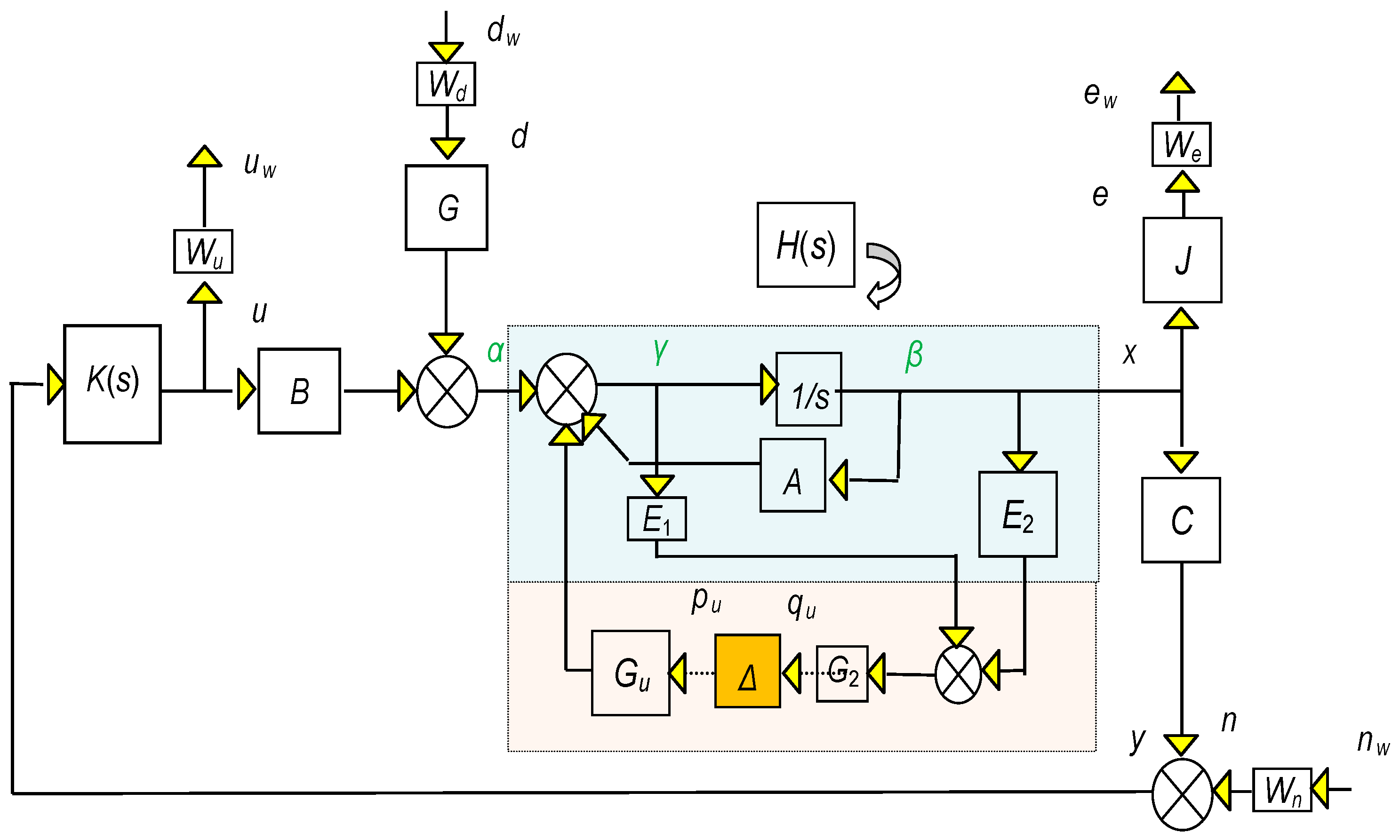
In this approach, we consider the original matrices’ uncertainty as an additional uncertainty factor. To convey our system in the form of Figure 4, consider Figure 13.

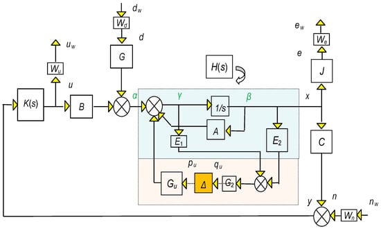
Figure 13. Uncertainty block diagram.

The matrices E₁, and E₂ are used to extract:

$$q_u\left(t\right)\stackrel{def}{=}\left[\begin{array}{c}\ddot{q}\left(t\right)\\ \dot{q}\left(t\right)\\ q\left(t\right)\end{array}\right].$$

Since

$$\gamma =\left[\begin{array}{c}\dot{q}\left(t\right)\\ \ddot{q}\left(t\right)\end{array}\right] \mathrm{and} \mathsf{\beta }=\int \left[\begin{array}{c}\dot{q}\left(t\right)\\ \ddot{q}\left(t\right)\end{array}\right]\mathrm{dt}=\left[\begin{array}{c}q\left(t\right)\\ \dot{q}\left(t\right)\end{array}\right],$$

appropriate choices for E₁ and E₂ are:

$${\mathrm{E}}_1=\left[\begin{array}{cc}{0}_{2\mathrm{n}\times 2\mathrm{n}}& {\mathrm{I}}_{2\mathrm{n}\times 2\mathrm{n}}\\ {\mathrm{I}}_{2\mathrm{n}\times 2\mathrm{n}}& 0_{2\mathrm{n}\times 2\mathrm{n}}\\ 0_{2\mathrm{n}\times 2\mathrm{n}}& 0_{2\mathrm{n}\times 2\mathrm{n}}\end{array}\right],\begin{array}{c} \end{array}{\mathrm{E}}_2=\left[\begin{array}{cc}{0}_{2\mathrm{n}\times 2\mathrm{n}}& 0_{2\mathrm{n}\times 2\mathrm{n}}\\ 0_{2\mathrm{n}\times 2\mathrm{n}}& 0_{2\mathrm{n}\times 2\mathrm{n}}\\ {\mathrm{I}}_{2\mathrm{n}\times 2\mathrm{n}}& 0_{2\mathrm{n}\times 2\mathrm{n}}\end{array}\right].$$

The idea is to find an N such that:

$$\left[\begin{array}{c}{q}_u\\ {\mathrm{e}}_{\mathrm{w}}\\ u_w\end{array}\right]=\mathrm{N}\left[\begin{array}{c}{\mathrm{p}}_{\mathrm{u}}\\ d_w\\ {\mathrm{n}}_{\mathrm{w}}\end{array}\right],\begin{array}{c} \end{array}\begin{array}{c}N=\end{array}\left[\begin{array}{ccc}{\mathrm{N}}_{{\mathrm{p}}_{\mathrm{u}}{\mathrm{q}}_{\mathrm{u}}}& {\mathrm{N}}_{{\mathrm{d}}_{\mathrm{w}}{\mathrm{q}}_{\mathrm{u}}}& {\mathrm{N}}_{{\mathrm{n}}_{\mathrm{w}}{\mathrm{q}}_{\mathrm{u}}}\\ {\mathrm{N}}_{{\mathrm{p}}_{\mathrm{u}}{\mathrm{e}}_{\mathrm{w}}}& {\mathrm{N}}_{{\mathrm{d}}_{\mathrm{w}}{\mathrm{e}}_{\mathrm{w}}}& {\mathrm{N}}_{{\mathrm{n}}_{\mathrm{w}}{\mathrm{e}}_{\mathrm{w}}}\\ {\mathrm{N}}_{{\mathrm{p}}_{\mathrm{u}}{\mathrm{u}}_{\mathrm{w}}}& {\mathrm{N}}_{{\mathrm{d}}_{\mathrm{w}}{\mathrm{u}}_{\mathrm{w}}}& {\mathrm{N}}_{{\mathrm{n}}_{\mathrm{w}}{\mathrm{u}}_{\mathrm{w}}}\end{array}\right]=\left[\begin{array}{cc}{\mathrm{N}}_{11}& {\mathrm{N}}_{12}\\ {\mathrm{N}}_{21}& {\mathrm{N}}_{22}\end{array}\right],$$

or in the notation of Figure 4,

$$\left[\begin{array}{c}{q}_u\\ w\end{array}\right]=\mathrm{N}\left[\begin{array}{c}{\mathrm{p}}_{\mathrm{u}}\\ z\end{array}\right].$$

Now ${\mathrm{N}}_{{\mathrm{d}}_{\mathrm{w}}{\mathrm{e}}_{\mathrm{w}}}$,${ \mathrm{N}}_{{\mathrm{ne}}_{\mathrm{w}}}$, ${\mathrm{N}}_{{\mathrm{d}}_{\mathrm{w}}{\mathrm{u}}_{\mathrm{w}}}$, and ${\mathrm{N}}_{{\mathrm{n}}_{\mathrm{w}}{\mathrm{u}}_{\mathrm{w}}}$ are known from Equation (28). For the rest, we will employ a method identified as “pulling out the Δ’s”. To this end, we split the loop at points p_u, and q_u (which will be employed as extra inputs/outputs correspondingly) and use the auxiliary signals α, β, and γ.

To obtain the transfer function ${\mathrm{N}}_{{\mathrm{d}}_{\mathrm{w}}\mathrm{qu}}$ (from d_w to q_u):

$$\begin{gathered} q_u={\mathrm{G}}_2({\mathrm{E}}_2\mathsf{\beta }+{\mathsf{{\rm E}}}_1\mathsf{\gamma })={\mathrm{G}}_2({\mathrm{E}}_2 \frac{1}{\mathrm{s}}+{\mathrm{E}}_1)\gamma \\ \gamma ={\mathrm{GW}}_{\mathrm{d}}{d}_w+\mathrm{B}u+\mathrm{A}\frac{1}{\mathrm{s}}\gamma ={\mathrm{GW}}_{\mathrm{d}}{\mathrm{d}}_{\mathrm{w}}+\mathrm{BKC}\frac{1}{\mathrm{s}}\gamma + \mathrm{A}\frac{1}{\mathrm{s}}\gamma \Rightarrow \gamma =(\mathrm{I}-\mathrm{BKC}\frac{1}{\mathrm{s}} -\mathrm{A}\frac{1}{\mathrm{s}}{)}^{-1}{\mathrm{GW}}_{\mathrm{d}}{d}_w \end{gathered}$$

Hence,

$${\mathrm{N}}_{{\mathrm{d}}_{\mathrm{w}}\mathrm{qu}}={\mathrm{G}}_2({\mathrm{E}}_2\frac{1}{\mathrm{s}}+{\mathrm{E}}_1)(\mathrm{I}-\mathrm{BKC}\frac{1}{\mathrm{s}} -\mathrm{A}\frac{1}{\mathrm{s}}{)}^{-1}{\mathrm{GW}}_{\mathrm{d}}$$

Now, ${\mathrm{N}}_{{\mathrm{p}}_{\mathrm{u}}{\mathrm{q}}_{\mathrm{u}}}$, ${\mathrm{N}}_{{\mathrm{p}}_{\mathrm{u}}{\mathrm{e}}_{\mathrm{w}}}$, and ${\mathrm{N}}_{{\mathrm{p}}_{\mathrm{u}}{\mathrm{u}}_{\mathrm{w}}}$ are similar to ${\mathrm{N}}_{{\mathrm{d}}_{\mathrm{w}}{\mathrm{q}}_{\mathrm{w}}}$ ${\mathrm{N}}_{{\mathrm{d}}_{\mathrm{w}}{\mathrm{e}}_{\mathrm{w}}}$, and ${\mathrm{N}}_{{\mathrm{d}}_{\mathrm{w}}{\mathrm{u}}_{\mathrm{w}}}$ with GW_d replaced by G_u, i.e.,

$${\mathrm{N}}_{{\mathrm{p}}_{\mathrm{u}}{\mathrm{q}}_{\mathrm{u}}}={\mathrm{G}}_2({\mathrm{E}}_2\frac{1}{\mathrm{s}}+{\mathrm{E}}_2)(\mathrm{I}-\mathrm{BKC}\frac{1}{\mathrm{s}}-\mathrm{A}\frac{1}{\mathrm{s}}{)}^{-1}{\mathrm{G}}_{\mathrm{u}},$$

$${\mathrm{N}}_{{\mathrm{p}}_{\mathrm{u}}{\mathrm{e}}_{\mathrm{w}}}={\mathrm{W}}_{\mathrm{y}}\mathrm{JH}[\mathrm{I}+\mathrm{B}[\mathrm{K}(\mathrm{I}-\mathrm{CHBK}{)}^{-1}\mathrm{CH}]{\mathrm{G}}_{\mathrm{u}},$$

$${\mathrm{M}}_{{\mathrm{p}}_{\mathrm{u}}{\mathrm{u}}_{\mathrm{w}} }={\mathrm{W}}_{\mathrm{U}}\mathrm{K}(\mathrm{I}-\mathrm{CHBK}{)}^{-1}\mathrm{CH}{\mathrm{G}}_{\mathrm{u}}.$$

Ultimately, to find ${\mathrm{N}}_{{\mathrm{n}}_{\mathrm{w}}{\mathrm{q}}_{\mathrm{u}}}$

$$\begin{gathered} q_u={\mathrm{G}}_2({\mathrm{E}}_2\mathsf{\beta }+{\mathsf{{\rm E}}}_1\gamma )={\mathrm{G}}_2({\mathrm{E}}_2\frac{1}{\mathrm{s}}+{\mathrm{E}}_1)\gamma \\ \gamma =\mathrm{Bu}+\mathrm{A}\frac{1}{\mathrm{s}}\gamma =\mathrm{BK}({\mathrm{W}}_{\mathrm{n}}{\mathrm{n}}_{\mathrm{w}}+\mathrm{y})+\mathrm{A}\frac{1}{\mathrm{s}}\gamma ={\mathrm{BKW}}_{\mathrm{n}}{\mathrm{n}}_{\mathrm{w}}+\mathrm{BKC}\frac{1}{\mathrm{s}}\gamma +\mathrm{A}\frac{1}{\mathrm{s}}\gamma \\ \Rightarrow \gamma =(\mathrm{I}-\mathrm{BKC}\frac{1}{\mathrm{s}} -\mathrm{A}\frac{1}{\mathrm{s}}{)}^{-1}{\mathrm{BKW}}_{\mathrm{n}}{\mathrm{n}}_{\mathrm{w}}. \end{gathered}$$

Hence,

$${\mathrm{N}}_{{\mathrm{n}}_{\mathrm{w}}{\mathrm{q}}_{\mathrm{u}}}={\mathrm{G}}_2({\mathrm{E}}_2\frac{1}{\mathrm{s}}+{\mathrm{E}}_1)(\mathrm{I}-\mathrm{BKC}\frac{1}{\mathrm{s}} -\mathrm{A}\frac{1}{\mathrm{s}}{)}^{-1}{\mathrm{BKW}}_{\mathrm{n}}.$$

Collecting all the above yields the transfer function of the structure N:

$$\left[\begin{array}{ccc}{G}_2\left(E_2\frac{1}{s}+E_1\right){\left(I-BKC\frac{1}{s}-A\frac{1}{s}\right)}^{-1}{G}_u& G_2\left(E_2\frac{1}{s}+E_1\right){\left(I-BKC\frac{1}{s}-A\frac{1}{s}\right)}^{-1}{GW}_d& G_2\left(E_2\frac{1}{s}+E_1\right){\left(I-BKC\frac{1}{s}-A\frac{1}{s}\right)}^{-1}{BKW}_n\\ W_{e}JH\left[I+BK{\left(I-CHBK\right)}^{-1}CF\right]G_u& W_{e}J{\left(I-HBKC\right)}^{-1}{HGW}_d& W_{e}J{\left(I-HBKC\right)}^{-1}{HBKW}_n\\ W_{u}K{\left(I-CHBK\right)}^{-1}{CFG}_u& W_u{\left(I-KCHB\right)}^{-1}{KCHGW}_d& W_u{\left(I-KCHB\right)}^{-1}KW\end{array}\right]$$

(33)

Having acquired N for the beam problem, all recommended controllers K(s) can be compared utilizing the constructed singular value relations. The above operations were calculated to find the transfer function (N) which is used in programming in the Matlab programming tool.

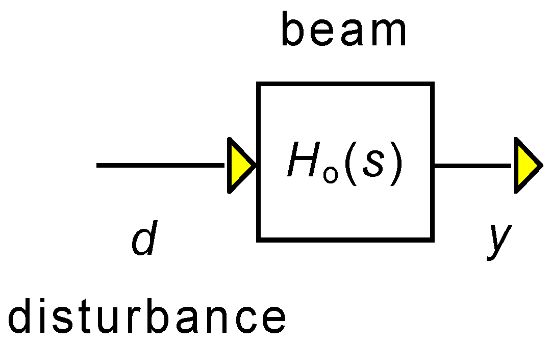
4.2. Results for the Open Loop (Initial Condition without Control)

The open loop system is displayed in Figure 14. Using Equations (2) and (3) the transfer function from disturbance to position is

H_o(s) = C(sI − A)⁻¹G.

(34)

Figure 14. Block diagram for the open loop.

The system is stable with the e-values of A at

1.0 × 10^0.007 ×

[−3.497882663196082

−1.371177496104841

−0.546611094980835

−0.215249175898536

−0.061335753206233

−0.015936656985647

−0.001837409669158

−0.000026475315963 + 0.000099444326281i

−0.000026475315963 − 0.000099444326281i

−0.000224428822398

−0.000202541835285

−0.000200654281462

−0.000200186003921

−0.000200011436140

−0.000200029176256

−0.000200073204937].

Firstly, we note that the A matrix is badly conditioned with condition number c = 5.62 × 10^−0.013. This means some preconditioning would be beneficial to sensitive calculations (like pole placement). A solution to this issue is to stabilize the system matrix. Matlab delivers the routine [36,37,38] [T, S] = balance(A) which creates a diagonal alteration matrix T whose elements are integer powers of 2, and matrix B such that

A = TST⁻¹.

As a result, some of the bad conditioning is transferred to T. Letting

z = T⁻¹x⇒x = Tz,

Equation (3) in the frequency domain, becomes:

$$\begin{array}{c} \mathrm{T}z\left(t\right)=\mathrm{AT}z\left(t\right)+\mathrm{B}u\left(t\right)+\mathrm{G}d\left(t\right)\\ \Rightarrow z\left(t\right)={\mathrm{T}}^{-1}\mathrm{AT}z\left(t\right)+{\mathrm{T}}^{-1}\mathrm{B}u\left(t\right)+{\mathrm{T}}^{-1}\mathrm{G}d\left(t\right)\\ =\mathrm{S}z\left(t\right)+\hat{\mathrm{B}}u\left(t\right)+\hat{\mathrm{G}}d\left(t\right).\end{array}$$

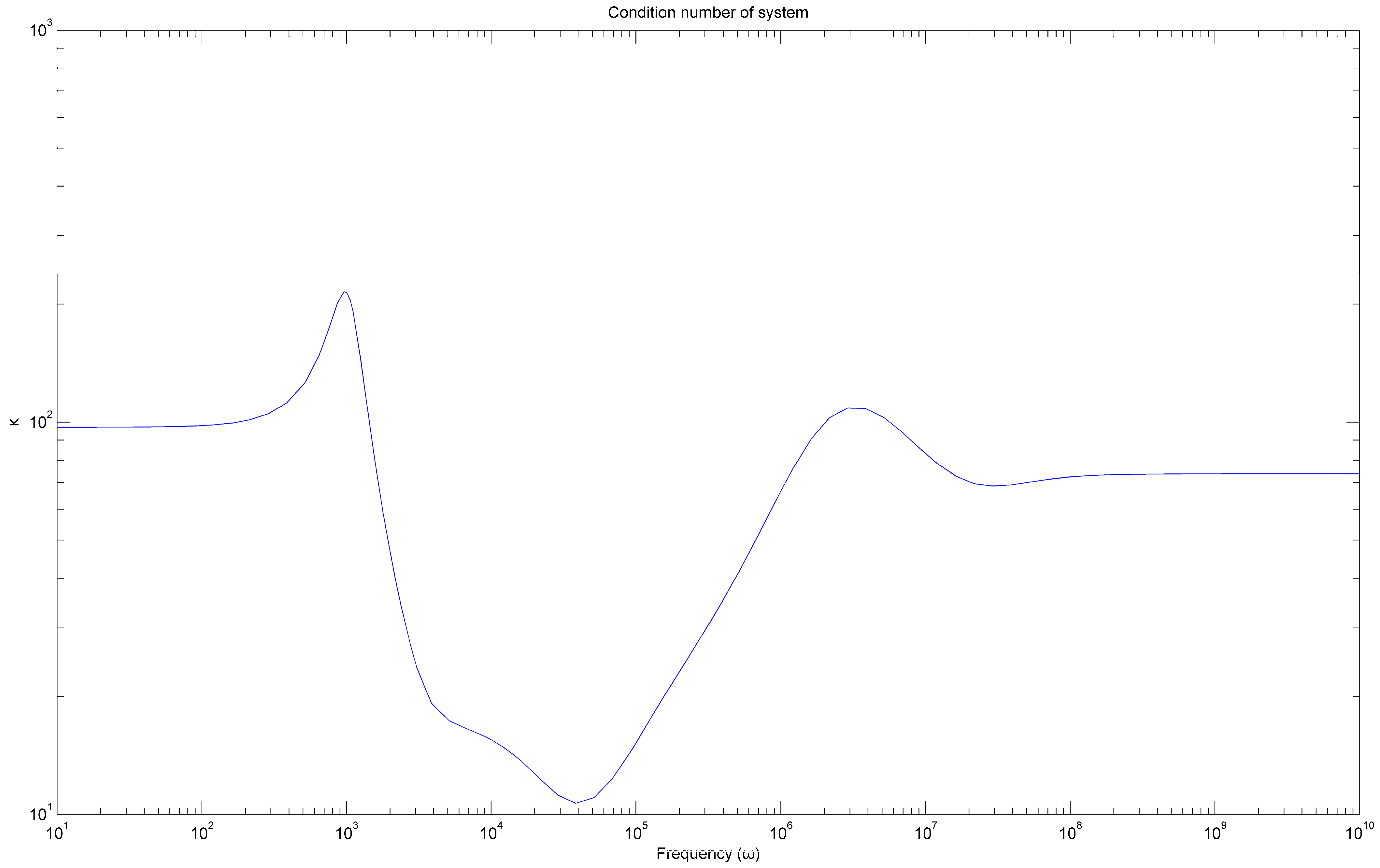
Another problem arises from the very small size of the minimum eigenvalue which defines the minimal time constant of the system, which in turn dictates sampling intervals used in simulations. These sampling intervals should be smaller than the minimum time constant. When this happens, arrays involved for example in lsim simulations become noticeably big, and particular care must be taken if the simulation time is large. Also, the system is both manageable and noticeable (in fact the system is both controllable and observable with fewer inputs and measurements). A probable measure of the difficulty of regulating the system is the frequency-dependent condition number κ(jω), defined by

$$\mathsf{\kappa }\left(\mathrm{j}\mathsf{\omega }\right)=\frac{\overline{\mathsf{\sigma }}\left({\mathrm{H}}_{\mathsf{o}}(\mathrm{j}\mathsf{\omega })\right)}{\underset{¯}{\mathsf{\sigma }}\left({\mathsf{H}}_{\mathsf{o}}(\mathrm{j}\mathsf{\omega })\right)}.$$

A high condition number implies that the system is “close” to losing its full rank, i.e., close to not fulfilling the property of operational controllability (that is the ability of the output to follow any preassigned trajectory over a provided time interval). Values close to 1 are desirable. Figure 15 shows the condition number for our system.

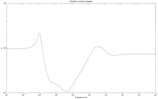
Figure 15. Condition number of the system.

As can be seen, the condition number is rather high at low frequencies, indicating that at those frequencies the system would be rather difficult to control [17,39,40]. This suggests that balancing would also be beneficial in this respect.

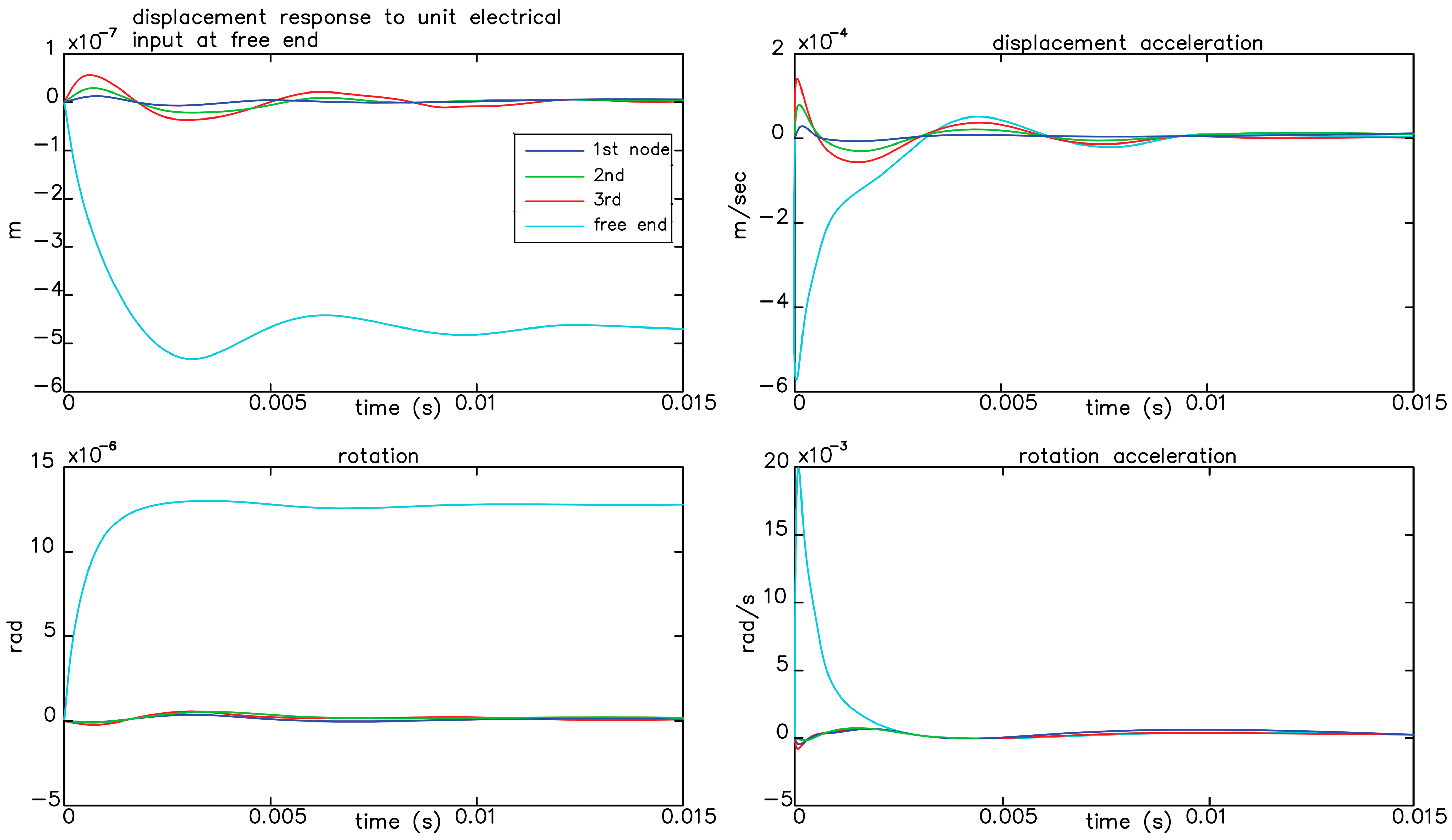
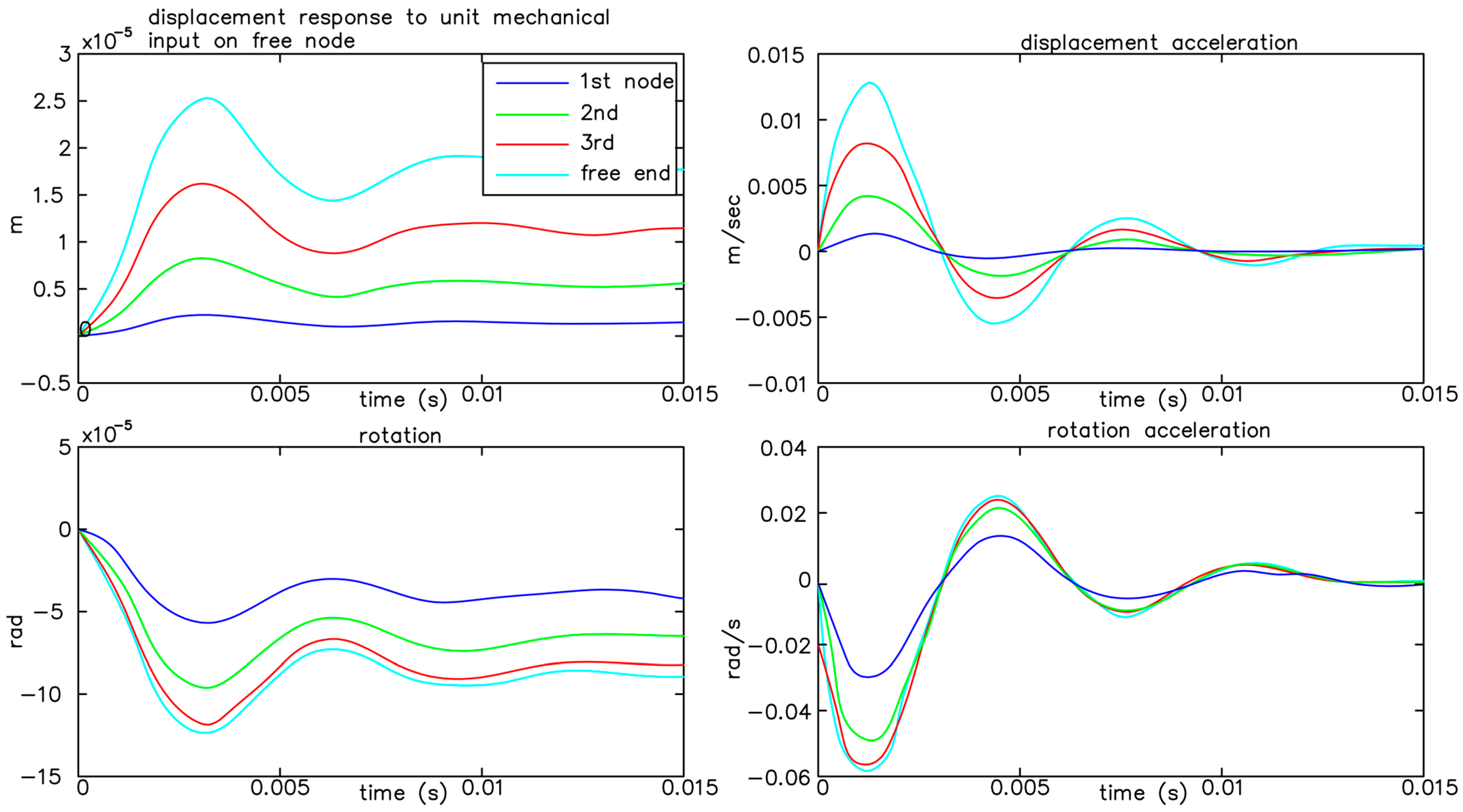
Responses to various inputs are in Figure 16, Figure 17 and Figure 18. These are Matlab simulations. These are simulations prior to applying the control in the beam. They are the initial conditions.

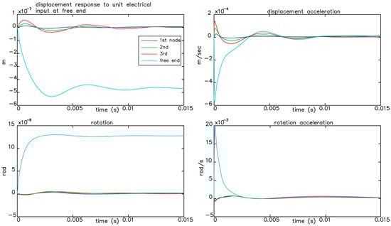
Figure 16. Responses for unit mechanical force for every node of the structure.

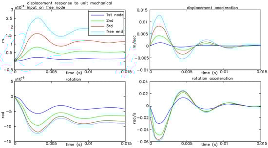
Figure 17. Responses for unit electrical force for every node of the structure.

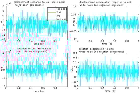
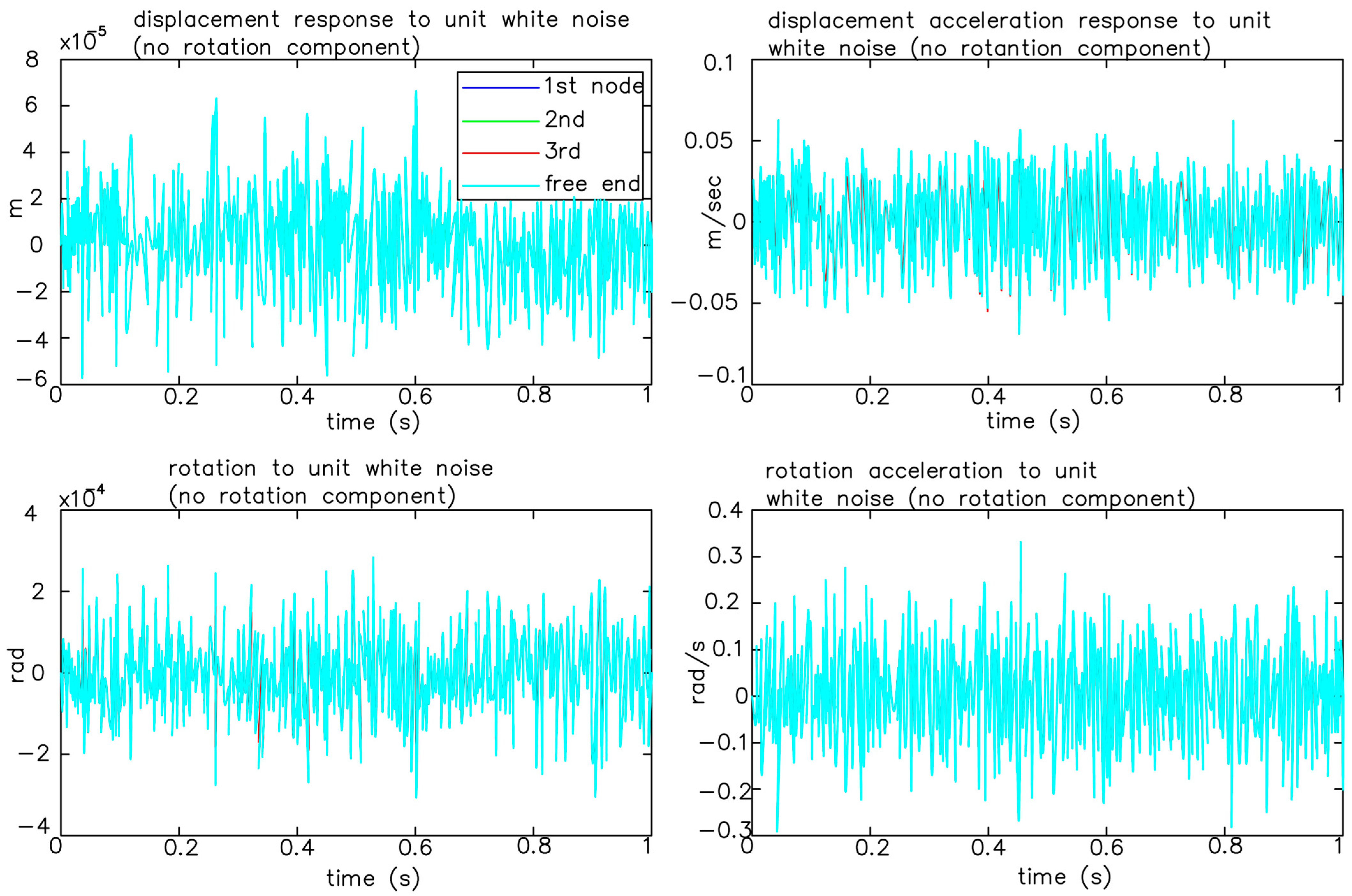
Figure 18. Responses for unit white noise for every node of the structure. The curves almost coincide; thus, the different curves cannot be clearly distinguished in the graphs.

In Figure 16 we see the responses of the structure for unit mechanical load 1 Ν, at each node of the model separately. Figure 17 shows the responses of the structure for unit electric 1 Volt charge while Figure 18 is for unit white noise. In this work, we achieve full suppression of oscillations with two control strategies, the Hinfinity control and the LQR. First, a smart structure is modeled with integrated piezoelectric elements that act as both sensors and actuators. Afterward, an optimal placement is made. Modeling uncertainties as well as measurement noise are taken into account, then advanced control techniques are applied. The results are presented both in the time domain and in the frequency domain.

4.3. Results with LQR Control

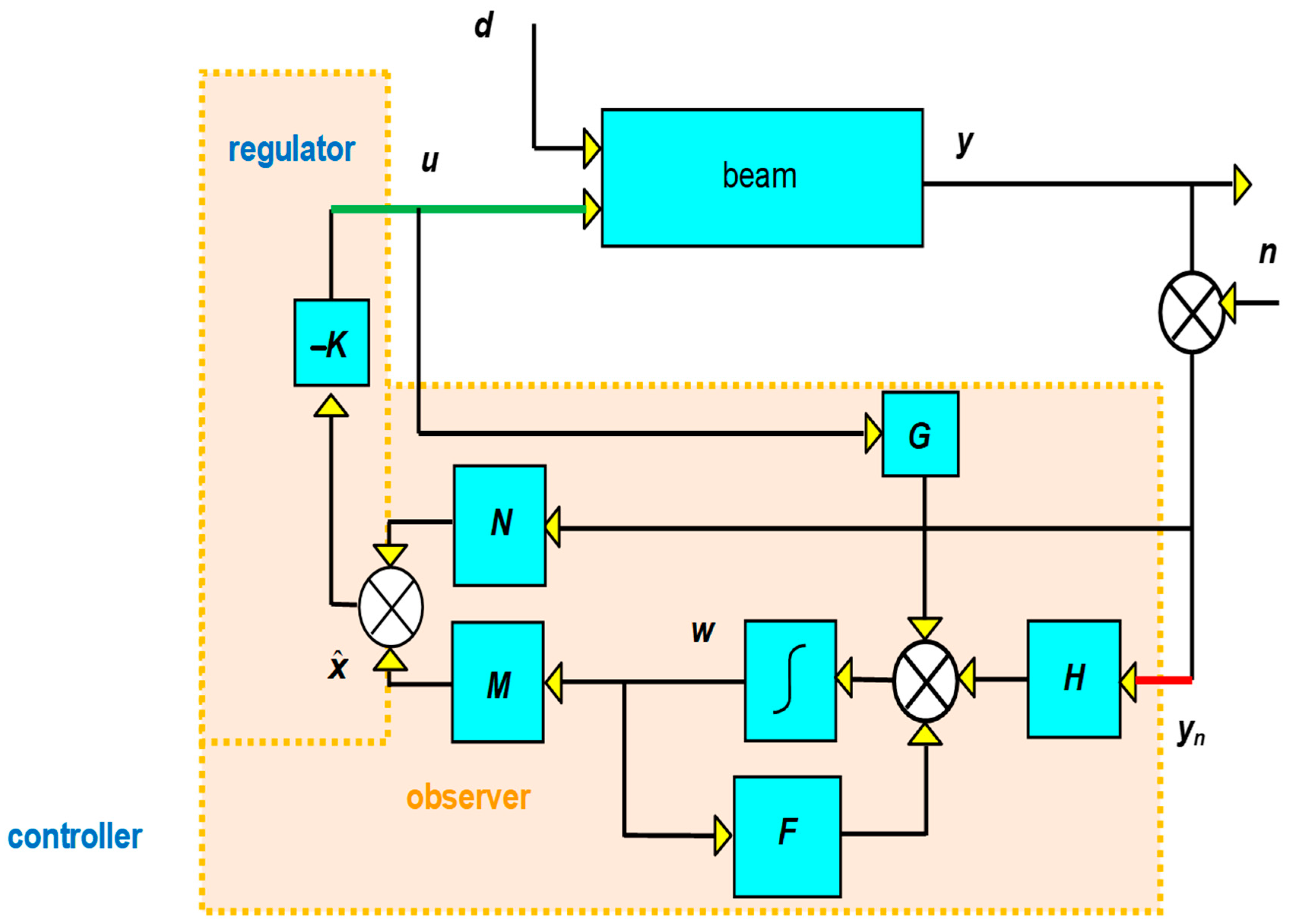
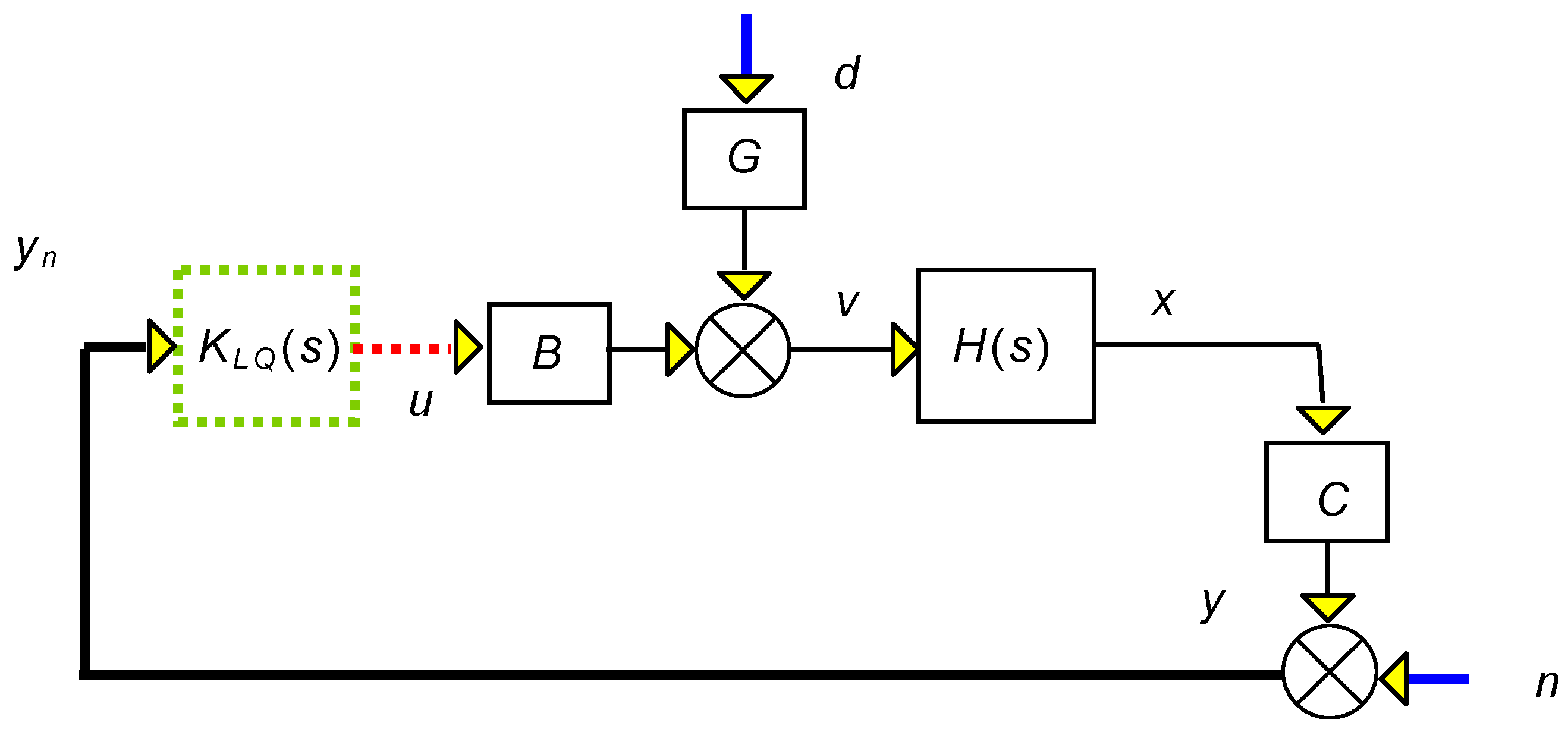
It is commonly known [41] that a controller must have a zero at infinity (i.e., integrate) to completely remove continuous input disturbances. An integrator’s role as a disturbance estimator is another helpful interpretation. Consequently, we do not anticipate an LQR controller to have a zero steady-state error. The structure of LQR control with diminished order observer is revealed in Figure 19.

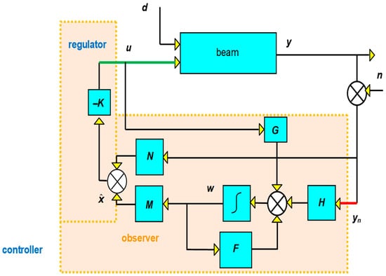
Figure 19. LQR controller with a state estimator.

Here,

$$\mathrm{K}=\underset{\mathrm{t}\to \infty }{\lim }\mathrm{K}\left(\mathrm{t}\right),$$

where:

$$u\left(t\right)=-\mathrm{K}\left(\mathrm{t}\right)\widehat{x}\left(t\right)$$

(35)

minimalizes the weighted performance index of

$$\mathrm{J}=\underset{0}{\overset{\infty }{{\displaystyle \int }}}\left({\widehat{x}}^T\left(t\right)\mathrm{Q}\widehat{x}\left(t\right)+u^T\left(t\right)\mathrm{R}u\left(t\right)\right)\mathrm{dt},$$

and Q and R are design weight matrices.

The necessary equations are:

$$\begin{gathered} {\left[\begin{array}{c}\mathrm{C}\\ \mathrm{T}\end{array}\right]}^{-1}=\left[\begin{array}{cc}\mathrm{P}& \mathrm{M}\end{array}\right],T\mathrm{arbitrary} \\ \left[\begin{array}{cc}\mathrm{CAP}& \mathrm{CAM}\\ \mathrm{TAP}& \mathrm{TAM}\end{array}\right]=\left[\begin{array}{cc}{\hat{\mathrm{A}}}_{11}& {\hat{\mathrm{A}}}_{12}\\ {\hat{\mathrm{A}}}_{21}& {\hat{\mathrm{A}}}_{22}\end{array}\right]\left[\begin{array}{c}\mathrm{CB}\\ \mathrm{TB}\end{array}\right]=\left[\begin{array}{c}{\hat{\mathrm{B}}}_1\\ {\hat{\mathrm{B}}}_2\end{array}\right] \\ \mathrm{F}={\hat{\mathrm{A}}}_{22}-\mathrm{L}{\hat{\mathrm{A}}}_{12}, \mathrm{H}=\mathrm{FL}+{\hat{\mathrm{A}}}_{21}-\mathrm{L}{\hat{\mathrm{A}}}_{11}, \mathrm{G}={\hat{\mathrm{B}}}_2-\mathrm{L}{\hat{\mathrm{B}}}_1,\mathrm{N}=\mathrm{P}+\mathrm{ML} \end{gathered}$$

$$\dot{\mathrm{w}}\left(\mathrm{t}\right)=\mathrm{Fw}\left(\mathrm{t}\right)+\mathrm{H}y\left(t\right)+\mathrm{G}u\left(t\right),$$

(36)

and

$$\widehat{x}\left(t\right)=\mathrm{Mw}\left(\mathrm{t}\right)+\mathrm{N}y\left(t\right).$$

(37)

Here matrix L is chosen to regulate:

$$\dot{z}\left(t\right)=\left[\begin{array}{cc}\mathsf{A}& 0\\ \mathrm{J}& 0\end{array}\right]z\left(t\right)+\left[\begin{array}{c}{\rm B}\\ 0\end{array}\right]\mathrm{v}\left(\mathrm{t}\right)$$

(38)

and

$$\dot{\tilde{z}}\left(t\right)=\left({\hat{\mathrm{A}}}_{22}-{\mathrm{L}\hat{\mathrm{A}}}_{12}\right)\tilde{z}\left(t\right).$$

(39)

The calculation is carried out by specifying the pole positions λ_L [42].

To compare structured μ values for the overall system, we need to express the LQR controller as a transfer function.

Let us find $\widehat{x}\left(s\right)$ using Equation (37).

Form Equation (36),

$$\dot{\mathrm{w}} \left(\mathrm{t}\right)=\mathrm{Fw}\left(\mathrm{t}\right)+Hy\left(t\right)+\mathrm{G}u\left(t\right)\Rightarrow \mathrm{sw}\left(\mathrm{s}\right)=\mathrm{Fw}\left(\mathrm{s}\right)+\mathrm{H}{y}_n\left(s\right)+\mathrm{G}u\left(s\right)$$

(40)

and

$$\Rightarrow \mathrm{w}\left(\mathrm{s}\right)={\left(\mathrm{sI}-\mathrm{F}\right)}^{-1}\left[\mathrm{H}{y}_n\left(s\right)+\mathrm{G}u\left(s\right)\right].$$

(41)

To find the input-output relation for the LQR controller use 41,

$$\begin{gathered} u\left(\mathrm{s}\right)=-\mathrm{K}\left\{\left[\mathrm{N}+\mathrm{M}{\left(\mathrm{sI}-\mathrm{F}\right)}^{-1}\mathrm{H}\right]y_n\left(s\right)+\mathrm{M}{\left(\mathrm{sI}-\mathrm{F}\right)}^{-1}\mathrm{G}u\left(s\right)\right\} \\ \Rightarrow \left[\mathrm{I}+\mathrm{KM}{\left(\mathrm{sI}-\mathrm{F}\right)}^{-1}\mathrm{G}\right]u\left(s\right)=-\mathrm{K}\left[\mathrm{N}+\mathrm{M}{\left(\mathrm{sI}-\mathrm{F}\right)}^{-1}\mathrm{H}\right]y_n\left(s\right) \end{gathered}$$

$$\Rightarrow u\left(s\right)=-{\left[\mathrm{I}+\mathrm{KM}{\left(\mathrm{sI}-\mathrm{F}\right)}^{-1}\mathrm{G}\right]}^{-1}\mathrm{K}\left[\mathrm{N}+\mathrm{M}{\left(\mathrm{sI}-\mathrm{F}\right)}^{-1}\mathrm{H}\right]y_n\left(s\right),$$

(42)

or

$$u\left(s\right)={\mathrm{K}}_{\mathrm{LQ}}{y}_n\left(s\right),$$

(43)

where:

$${\mathrm{K}}_{\mathrm{LQ}}=-{\left[\mathrm{I}+\mathrm{KM}{\left(\mathrm{sI}-\mathrm{F}\right)}^{-1}\mathrm{G}\right]}^{-1}\mathrm{K}\left[\mathrm{N}+\mathrm{M}{\left(\mathrm{sI}-\mathrm{F}\right)}^{-1}\mathrm{H}\right].$$

(44)

With this relation, our LQR control structure can be depicted more compactly as shown in Figure 20,

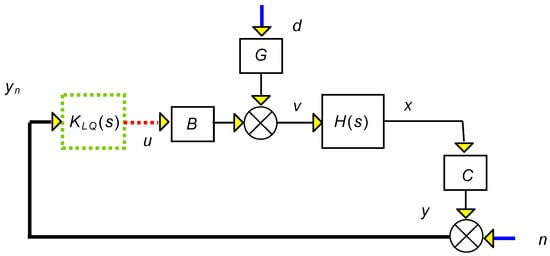
Figure 20. Beam LQR control.

Where H(s) = (sI − A)⁻¹ is the beam’s transfer function.

Matrix L is a design matrix. Its e-values are chosen so that the observer subsystem is about twice as fast as the observed plant. For our simulations we used

$$\begin{gathered} {\Lambda }_{\mathrm{L}}=1.0\times {10}^{0.007}\times \\ \left[\begin{array}{ccc}2.7423 & -0.4304 & \begin{array}{ccc}-0.0318 & -0.000051+0.002i& \begin{array}{ccc}-0.000051-0.002i& -0.00045+0.000053i& \begin{array}{ccc}-0.00045-0.000053i& -0.00039+0.00001i& \begin{array}{ccc}-0.00039-0.00001i& -0.000401 & \begin{array}{cc}-0,0004003& -0.0004004\end{array}\end{array}\end{array}\end{array}\end{array}\end{array}\right]T. \end{gathered}$$

These values were found by trial and error, given the bad numerical properties of the system. Furthermore, a robust pole placement algorithm, implemented in Matlab was used.

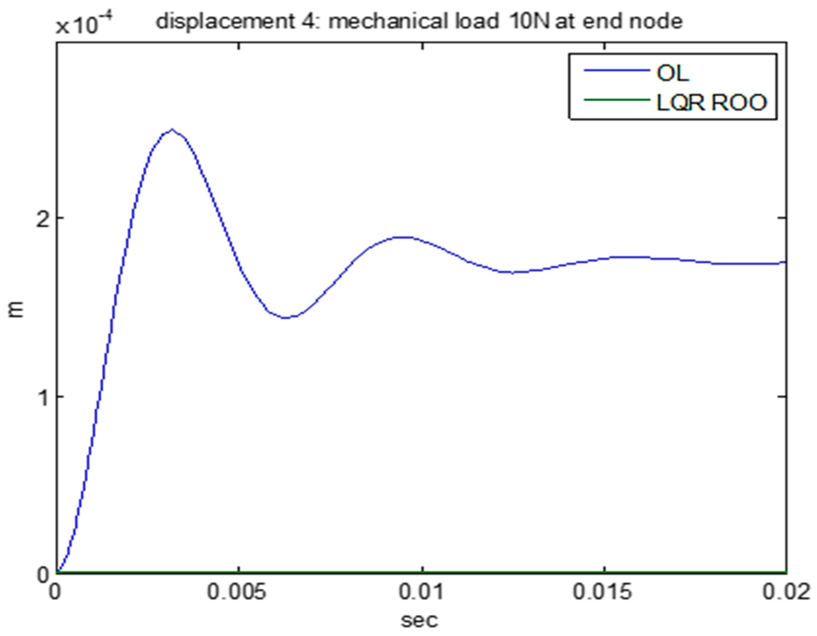
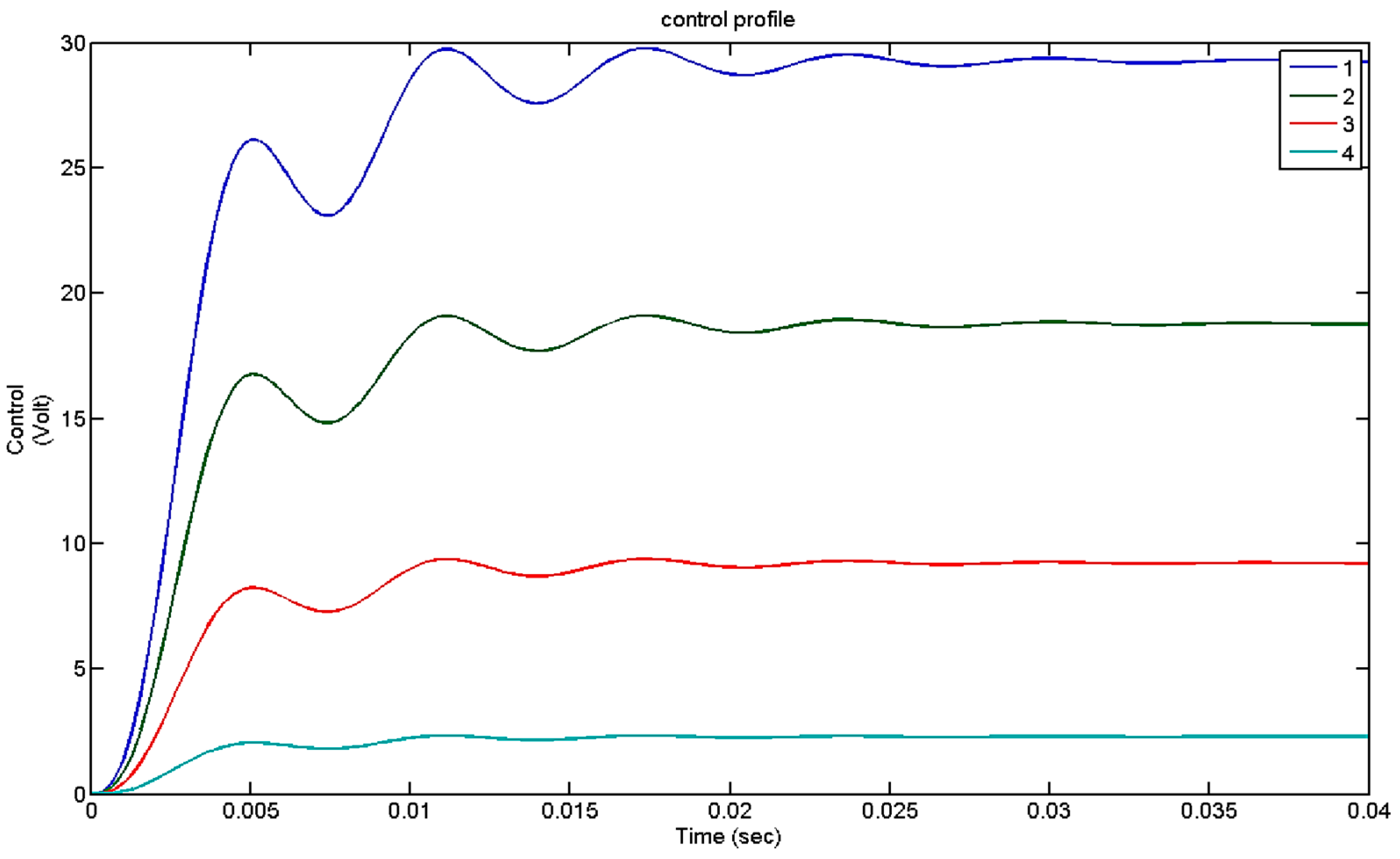
In the simulations, artificial noise of amplitude equal to a random percentage (in the interval −1 to +1) of the measured values was added. The results of the simulations are shown in Figure 21 and Figure 22. The results presented are for the second case of actuator placement. In Figure 21 we can witness the dislocation of the free end of the beam with control (closed loop, green line) and without control (open loop, blue line) when the mechanical force is 10 N at the free end of the constructs. The displacement for the closed loop is almost zero. In Figure 22 we can notice the control voltages for the previous closed-loop displacements. The piezoelectric limits are 500 Volts and the control voltages we used are 30 Volts.

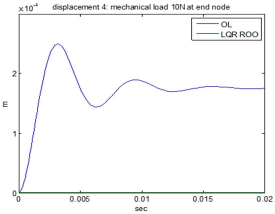
Figure 21. LQR reduced order observer controller: displacement at the end node.

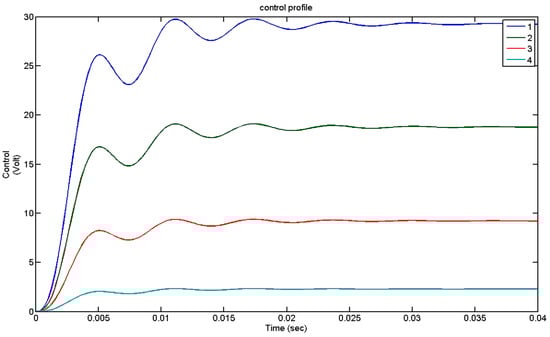
Figure 22. LQR reduced order observer controller: control effort.

4.4. Results with Hinfinity Control

Various tests were performed. We expect to improve our performance if we exploit the frequency dependence of the signals [43].

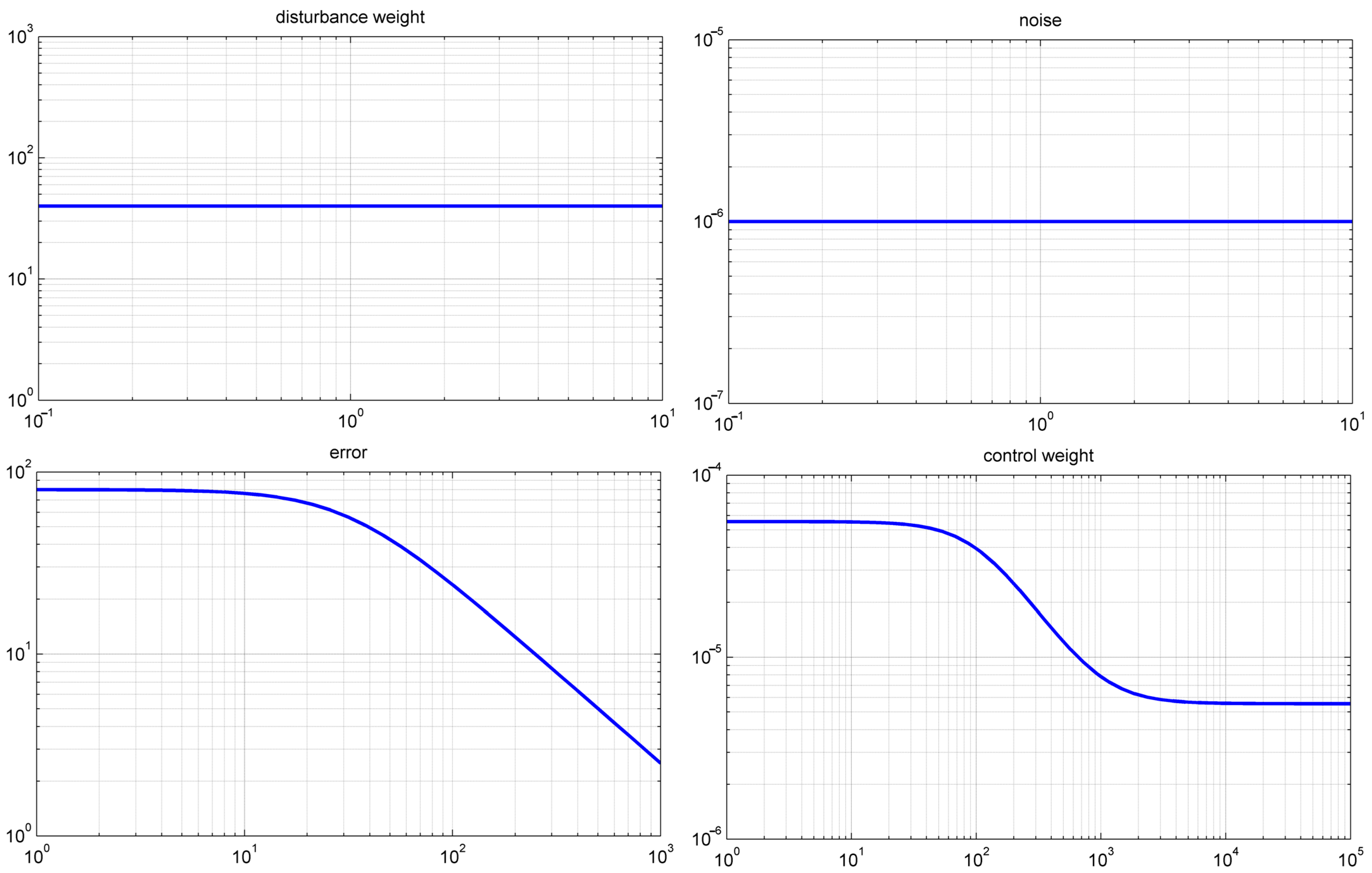
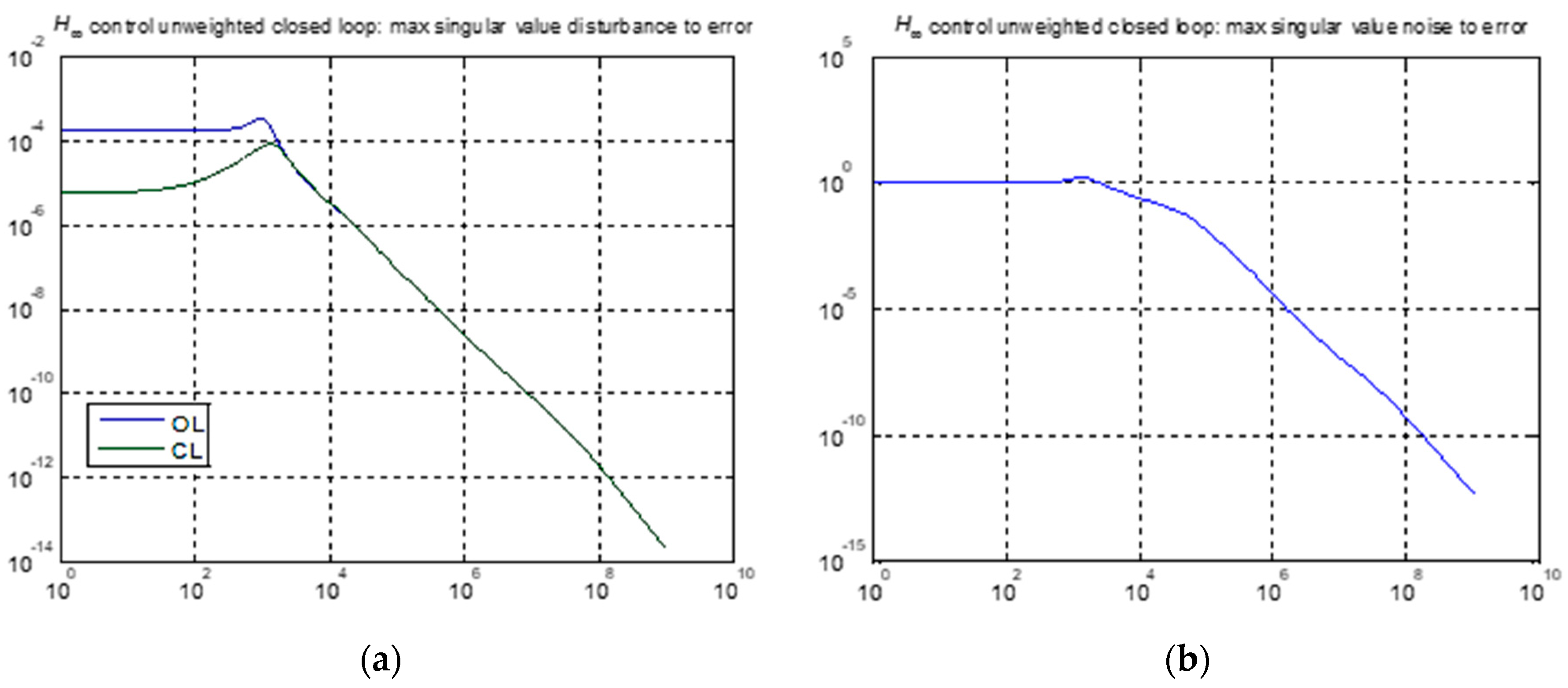
Figure 23 shows the Bode diagrams of the diagonal elements of the weight matrixes of H_infinity control, where the matrixes have been obtained after optimization. Nominal performance is depicted in Figure 24, Figure 25, Figure 26, Figure 27 and Figure 28. The resulting controller is order 36. The max singular value for this controller is 0.074. In Figure 24b the performance of the controller is significant since it appears that there is a significant improvement in the error noise for frequencies above 1000 Hz. Moreover, Figure 24a shows the noteworthy enhancement of the effect of disturbances on the error up to the frequency of 1000 Hz.

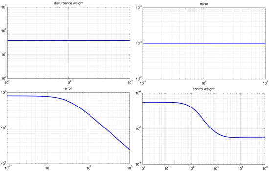
Figure 23. Bode diagrams.

Figure 24. H_∞ control: max singular value plots for the closed loop unweighted system’s error (a) disturbance to error, (b) noise to error.

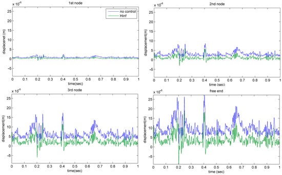
Figure 25. Displacement for the first place of piezoelectric patches.

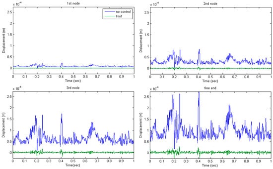
Figure 26. Displacement for the second place of piezoelectric patches.

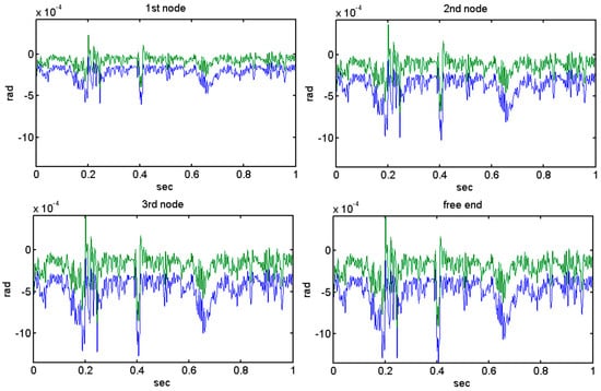
Figure 27. Rotation for the second place of piezoelectric patches; Blue line—no control; Green line—Hinf.

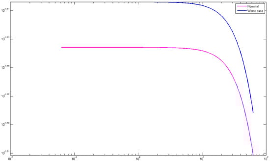
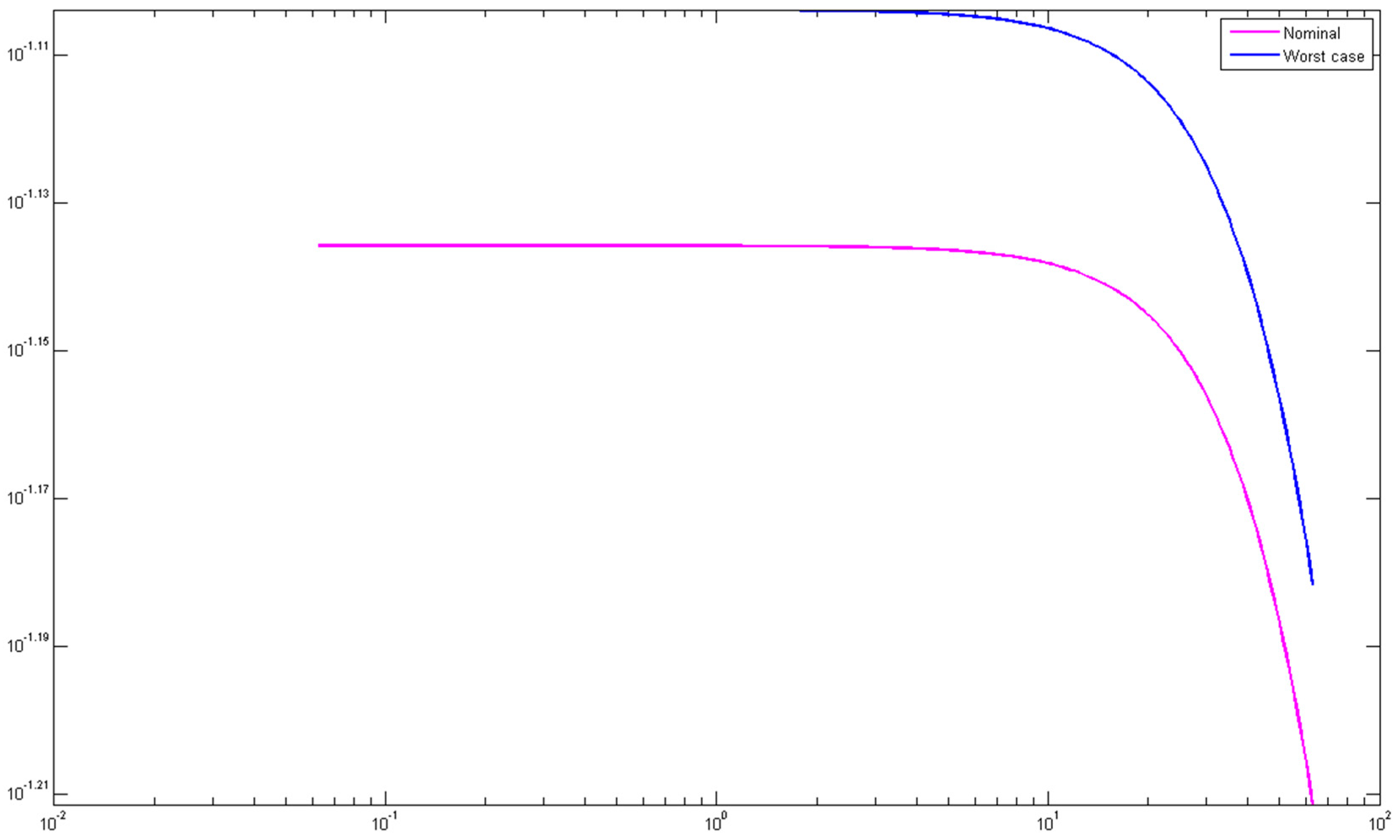
Figure 28. Singular values for the nominal and the worst case of the structures.

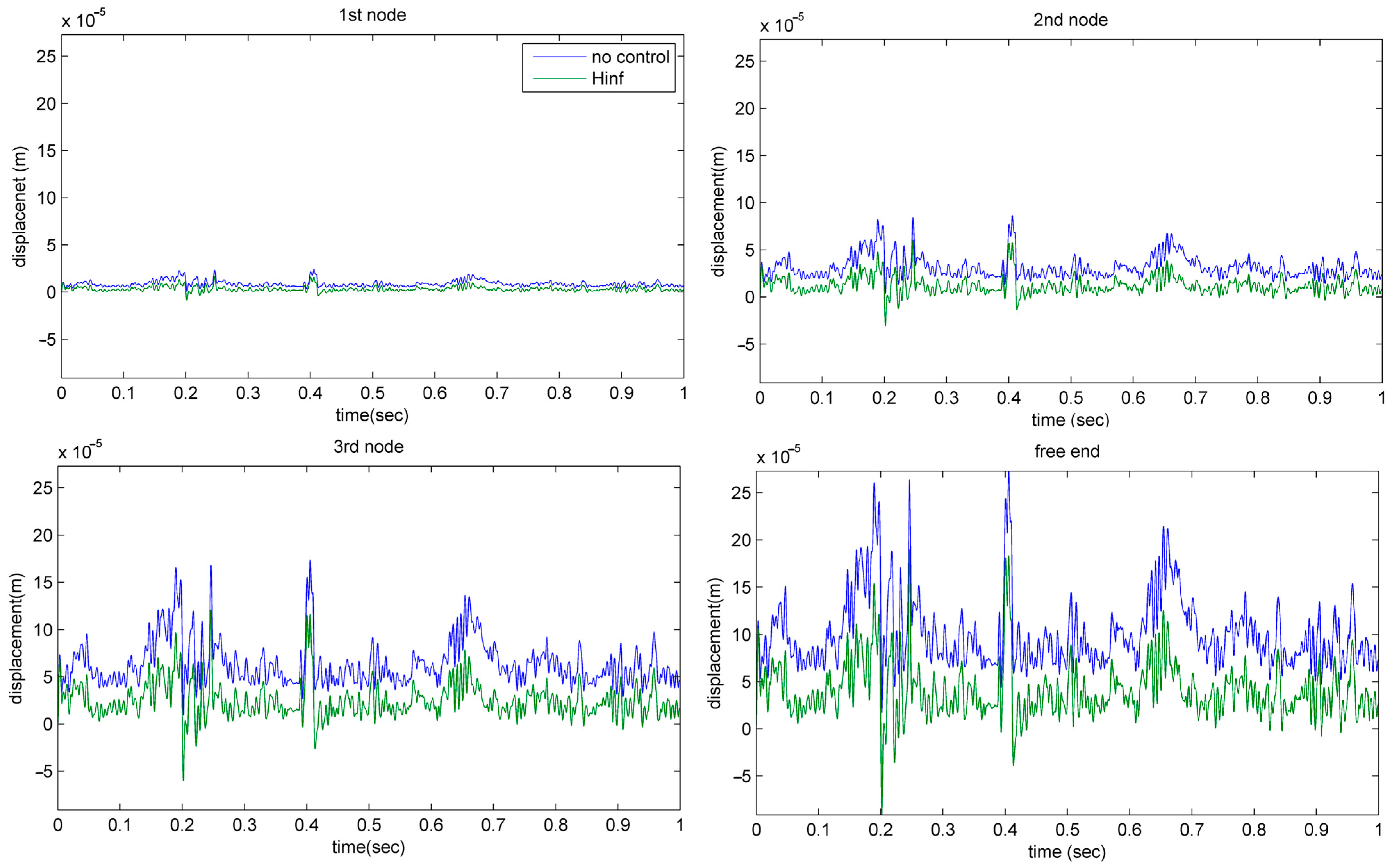
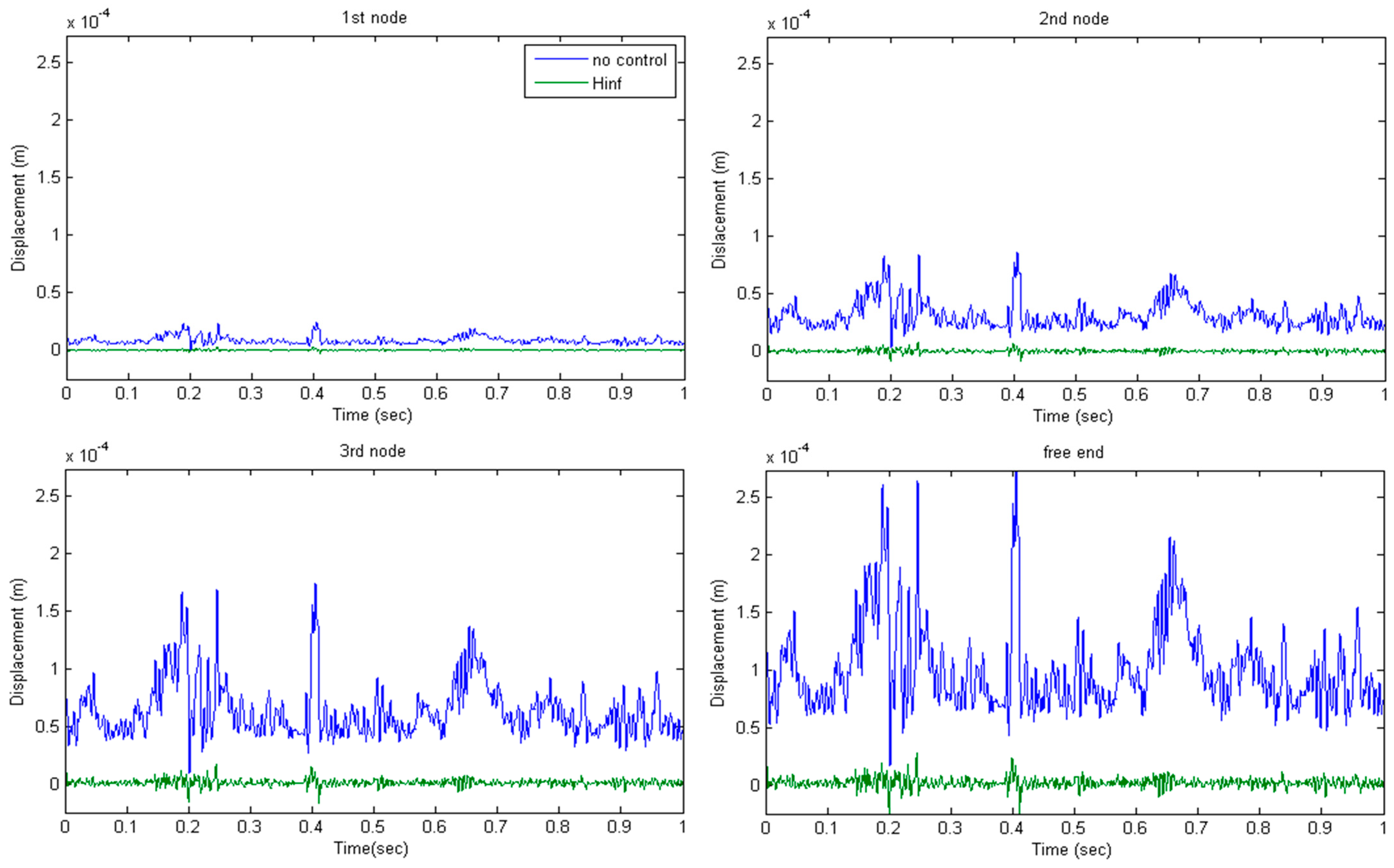
For all the next simulations a dynamical mechanical force is used, a real wind force which is taken from the Hellenic Mediterranean University in Heraklion, Crete in the energy laboratory of the Mechanical Engineering Department. In Figure 25 we can see the displacement for the first places of piezoelectric patches with and without control (Figure 1 and Figure 3). The blue line is the displacement without control (open loop), and the green line is the displacement with control (closed loop). In Figure 26 we have the same diagram for different places of the piezoelectric patches for all the nodes of the structures (Figure 2 and Figure 4). The results are excellent; the displacement is almost zero and the beam keeps in equilibrium. In Figure 27 we take the rotation for the second placement of the piezoelectric patches with (green line) Hinfinity control and without control (blue line). The results are excellent. In order to achieve them, the weights used had to be selected using optimization methods. Figure 28 shows the Singular values for the nominal and the worst case of the structures.

5. Discussion

In this study, detailed modeling of the problem of smart beam oscillation suppression is performed. It is shown in an analytical way the introduction of uncertainty into the model and the creation of the transfer function for the specific problem. The results are obtained after programming in the Matlab platform and using the Simulink software tool.

Control theory employing Hinfinity (H_∞) techniques is used to synthesize controllers for stabilization with assured performance. By expressing the control problem as a mathematical optimization problem and then identifying the controller that resolves this optimization, a control designer can employ Hinfinity techniques. In comparison to classical control techniques, H_∞ techniques have the advantage of being easily adaptable to problems involving multivariate systems with cross-coupling between channels. Hinfinity techniques’ drawbacks include the level of mathematical sophistication required for successful application and the requirement for a passably accurate model of the system to be controlled. Keep in mind that the resultant controller may not always be the best and is just the optimum solution with regard to the required cost function. The closed-loop impact of a perturbation may be reduced using H_∞ methods. Depending on how the problem is phrased, the impact will either be assessed in terms of stability or performance. The issue of control in intelligent structures has been addressed by a number of significant researchers [23,24,25]. While the modeling of the vector and the thorough suppression of oscillations are provided in detail in our research, the challenge of topological optimization of structures is covered in this study [25].

The article has made a great contribution to the following:

• On the modeling of uncertainty in smart constructions.
• In the creation of advanced control techniques.
• In the complete suppression of vibrations under dynamic loading.
• Analytical explanation of the equations used in programming.
• Advanced programming techniques have been used to make the simulations.
• The model has been worked both in simulation and in advanced programming.
• It is not possible in one article to present both the modeling and the experimental results in such detail. For this reason, they will be presented in future research papers.

In this article, we wanted to emphasize the analysis and composition of the beam model in an analytical way and for this reason, all equations are given in detail. It is very difficult to give the experimental results as well because it will greatly increase the size of the work.

6. Conclusions

Combining LQR and Hinfinity control, this research investigates the ideal positioning of actuators in intelligent structures. The resistance of the Hinfinity controller to parametric uncertainty is seen in problems with vibration suppression. The benefits of active vibration suppression and robust control in the dynamics of intelligent structures are well illustrated in this work. Hinfinity control has a number of advantages when examining dependable control systems. Hinfinity control allows for the minimization of oscillations even for different places of actuators. Numerical modeling shows that the recommended methods for reducing vibrations in piezoelectric smart structures are successful. By demonstrating the use of Hinfinity regulation in both the frequency domain and state space, this essay explored the benefits of robust control in intelligent architecture. There are a number of papers considering the optimal placement of actuators. Most of them are neglected in the literature review [23,24,25].

To conclude, this work has contributed to the following:

-

Modeling of intelligent constructs execution of control in oscillation suppression.

-

Using various choice places to stifle oscillations.

-

Results in the frequency domain as well as the time-space domain.

-

Introduction of the uncertainties in the construction’s mathematical model.

-

The integration of smart structures using methods for optimal placement and active control.

-

Uncertainties in dynamic loading.

-

Measurement noise, appropriate selection of weights for complete suppression of oscillations.

The application to simpler models allows the application of advanced control techniques since the controller presented is of order 36. All simulations have been conducted in Matlab with advanced programming techniques. Experimental investigation was not of the interest of this paper. All equations are provided in detail because the goal of this research was to stress the analysis and composition of the beam model using a very analytical approach. Giving experimental data is highly challenging since it will significantly lengthen the process.

References

- Tzou, H.S.; Gabbert, U. Structronics—A New Discipline and Its Challenging Issues. Fortschr.-Berichte VDI Smart Mech. Syst.—Adapt. Reihe 1997, 11, 245–250. [Google Scholar]
- Guran, A.; Tzou, H.-S.; Anderson, G.L.; Natori, M.; Gabbert, U.; Tani, J.; Breitbach, E. Structronic Systems: Smart Structures, Devices and Systems; World Scientific: Singapore, 1998; Volume 4, ISBN 978-981-02-2652-7. [Google Scholar]
- Tzou, H.S.; Anderson, G.L. Intelligent Structural Systems; Springer: London, UK, 1992; ISBN 978-94-017-1903-2. [Google Scholar]
- Gabbert, U.; Tzou, H.S. IUTAM Symposium on Smart Structures and Structronic Systems. In Proceedings of the IUTAM Symposium, Magdeburg, Germany, 26–29 September 2000; Kluwer: London, UK, 2001. [Google Scholar]
- Tzou, H.S.; Natori, M.C. Piezoelectric Materials and Continua; Elsevier: Oxford, UK, 2001; pp. 1011–1018. ISBN 978-0-12-227085-7. [Google Scholar]
- Cady, W.G. Piezoelectricity: An Introduction to the Theory and Applications of Electromechanical Phenomena in Crystals; Dover Publication: New York, NY, USA, 1964. [Google Scholar]
- Tzou, H.S.; Bao, Y. A Theory on Anisotropic Piezothermoelastic Shell Laminates with Sensor/Actuator Applications. J. Sound Vib. 1995, 184, 453–473. [Google Scholar] [CrossRef]
- Bikas, H.; Stavropoulos, P.; Chryssolouris, G. Additive Manufacturing Methods and Modelling Approaches: A Critical Review. Int. J. Adv. Manuf. Technol. 2016, 83, 389–405. [Google Scholar] [CrossRef]
- Stavropoulos, P.; Chantzis, D.; Doukas, C.; Papacharalampopoulos, A.; Chryssolouris, G. Monitoring and Control of Manufacturing Processes: A Review. Procedia CIRP 2013, 8, 421–425. [Google Scholar] [CrossRef]
- Vidakis, N.; Petousis, M.; Mountakis, N.; Papadakis, V.; Moutsopoulou, A. Mechanical Strength Predictability of Full Factorial, Taguchi, and Box Behnken Designs: Optimization of Thermal Settings and Cellulose Nanofibers Content in PA12 for MEX AM. J. Mech. Behav. Biomed. Mater. 2023, 142, 105846. [Google Scholar] [CrossRef] [PubMed]
- David, C.; Sagris, D.; Petousis, M.; Nasikas, N.K.; Moutsopoulou, A.; Sfakiotakis, E.; Mountakis, N.; Charou, C.; Vidakis, N. Operational Performance and Energy Efficiency of MEX 3D Printing with Polyamide 6 (PA6): Multi-Objective Optimization of Seven Control Settings Supported by L27 Robust Design. Appl. Sci. 2023, 13, 8819. [Google Scholar] [CrossRef]
- Moutsopoulou, A.; Stavroulakis, G.E.; Petousis, M.; Vidakis, N.; Pouliezos, A. Smart Structures Innovations Using Robust Control Methods. Appl. Mech. 2023, 4, 856–869. [Google Scholar] [CrossRef]
- Cen, S.; Soh, A.-K.; Long, Y.-Q.; Yao, Z.-H. A New 4-Node Quadrilateral FE Model with Variable Electrical Degrees of Freedom for the Analysis of Piezoelectric Laminated Composite Plates. Compos. Struct. 2002, 58, 583–599. [Google Scholar] [CrossRef]
- Yang, S.M.; Lee, Y.J. Optimization of Noncollocated Sensor/Actuator Location and Feedback Gain in Control Systems. Smart Mater. Struct. 1993, 2, 96. [Google Scholar] [CrossRef]
- Ramesh Kumar, K.; Narayanan, S. Active Vibration Control of Beams with Optimal Placement of Piezoelectric Sensor/Actuator Pairs. Smart Mater. Struct. 2008, 17, 55008. [Google Scholar] [CrossRef]
- Hanagud, S.; Obal, M.W.; Calise, A.J. Optimal Vibration Control by the Use of Piezoceramic Sensors and Actuators. J. Guid. Control Dyn. 1992, 15, 1199–1206. [Google Scholar] [CrossRef]
- Song, G.; Sethi, V.; Li, H.-N. Vibration Control of Civil Structures Using Piezoceramic Smart Materials: A Review. Eng. Struct. 2006, 28, 1513–1524. [Google Scholar] [CrossRef]
- Bandyopadhyay, B.; Manjunath, T.C.; Umapathy, M. Modeling, Control and Implementation of Smart Structures a FEM-State Space Approach; Springer: Berlin/Heidelberg, Germany, 2007; ISBN 978-3-540-48393-9. [Google Scholar]
- Miara, B.; Stavroulakis, G.E.; Valente, V. Topics on Mathematics for Smart Systems. In Proceedings of the European Conference, Rome, Italy, 26–28 October 2006. [Google Scholar]
- Moutsopoulou, A.; Stavroulakis, G.E.; Pouliezos, A.; Petousis, M.; Vidakis, N. Robust Control and Active Vibration Suppression in Dynamics of Smart Systems. Inventions 2023, 8, 47. [Google Scholar] [CrossRef]
- Zhang, N.; Kirpitchenko, I. Modelling Dynamics of a Continuous Structure with a Piezoelectric Sensoractuator for Passive Structural Control. J. Sound Vib. 2002, 249, 251–261. [Google Scholar] [CrossRef]
- Stavropoulos, P.; Manitaras, D.; Papaioannou, C.; Souflas, T.; Bikas, H. Development of a Sensor Integrated Machining Vice Towards a Non-Invasive Milling Monitoring System BT-Flexible Automation and Intelligent Manufacturing: The Human-Data-Technology Nexus; Kim, K.-Y., Monplaisir, L., Rickli, J., Eds.; Springer International Publishing: Cham, Switzerland, 2023; pp. 29–37. [Google Scholar]
- Baz, A.; Poh, S. Performance of an Active Control System with Piezoelectric Actuators. J. Sound Vib. 1988, 126, 327–343. [Google Scholar] [CrossRef]
- Moretti, M.; Silva, E.C.N.; Reddy, J.N. Topology Optimization of Flextensional Piezoelectric Actuators with Active Control Law. Smart Mater. Struct. 2019, 28, 35015. [Google Scholar] [CrossRef]
- Ma, X.; Wang, Z.; Zhou, B.; Xue, S. A Study on Performance of Distributed Piezoelectric Composite Actuators Using Galerkin Method. Smart Mater. Struct. 2019, 28, 105049. [Google Scholar] [CrossRef]
- Stavropoulos, P. Digitization of Manufacturing Processes: From Sensing to Twining. Technologies 2022, 10, 98. [Google Scholar] [CrossRef]
- Stavropoulos, P.; Souflas, T.; Papaioannou, C.; Bikas, H.; Mourtzis, D. An Adaptive, Artificial Intelligence-Based Chatter Detection Method for Milling Operations. Int. J. Adv. Manuf. Technol. 2023, 124, 2037–2058. [Google Scholar] [CrossRef]
- Ward, R.; Sun, C.; Dominguez-Caballero, J.; Ojo, S.; Ayvar-Soberanis, S.; Curtis, D.; Ozturk, E. Machining Digital Twin Using Real-Time Model-Based Simulations and Lookahead Function for Closed Loop Machining Control. Int. J. Adv. Manuf. Technol. 2021, 117, 3615–3629. [Google Scholar] [CrossRef]
- Afazov, S.; Scrimieri, D. Chatter Model for Enabling a Digital Twin in Machining. Int. J. Adv. Manuf. Technol. 2020, 110, 2439–2444. [Google Scholar] [CrossRef]
- Zhang, X.; Shao, C.; Li, S.; Xu, D.; Erdman, A.G. Robust H∞ Vibration Control for Flexible Linkage Mechanism Systems with Piezoelectric Sensors and Actuators. J. Sound Vib. 2001, 243, 145–155. [Google Scholar] [CrossRef]
- Packard, A.; Doyle, J.; Balas, G. Linear, Multivariable Robust Control with a μ Perspective. J. Dyn. Syst. Meas. Control 1993, 115, 426–438. [Google Scholar] [CrossRef]
- Stavroulakis, G.E.; Foutsitzi, G.; Hadjigeorgiou, E.; Marinova, D.; Baniotopoulos, C.C. Design and Robust Optimal Control of Smart Beams with Application on Vibrations Suppression. Adv. Eng. Softw. 2005, 36, 806–813. [Google Scholar] [CrossRef]
- Kimura, H. Robust Stabilizability for a Class of Transfer Functions. IEEE Trans. Autom. Control 1984, 29, 788–793. [Google Scholar] [CrossRef]
- Burke, J.V.; Henrion, D.; Lewis, A.S.; Overton, M.L. Stabilization via Nonsmooth, Nonconvex Optimization. IEEE Trans. Autom. Control 2006, 51, 1760–1769. [Google Scholar] [CrossRef]
- Doyle, J.; Glover, K.; Khargonekar, P.; Francis, B. State-Space Solutions to Standard H2 and H∞ Control Problems. In Proceedings of the 1988 American Control Conference, Atlanta, GA, USA, 15–17 June 1988; pp. 1691–1696. [Google Scholar]
- Francis, B.A. A Course in H∞ Control Theory; Springer: Berlin/Heidelberg, Germany, 1987; ISBN 978-3-540-17069-3. [Google Scholar]
- Friedman, Z.; Kosmatka, J.B. An Improved Two-Node Timoshenko Beam Finite Element. Comput. Struct. 1993, 47, 473–481. [Google Scholar] [CrossRef]
- Tiersten, H.F. Linear Piezoelectric Plate Vibrations: Elements of the Linear Theory of Piezoelectricity and the Vibrations Piezoelectric Plates, 1st ed.; Springer: New York, NY, USA, 1969; ISBN 978-1-4899-6221-8. [Google Scholar]
- Turchenko, V.A.; Trukhanov, S.V.; Kostishin, V.G.; Damay, F.; Porcher, F.; Klygach, D.S.; Vakhitov, M.G.; Lyakhov, D.; Michels, D.; Bozzo, B.; et al. Features of Structure, Magnetic State, and Electrodynamic Performance of SrFe12−xInxO19. Sci. Rep. 2021, 11, 18342. [Google Scholar] [CrossRef]
- Kwakernaak, H. Robust Control and H∞-Optimization—Tutorial Paper. Automatica 1993, 29, 255–273. [Google Scholar] [CrossRef]
- Chandrashekhara, K.; Varadarajan, S. Adaptive Shape Control of Composite Beams with Piezoelectric Actuators. J. Intell. Mater. Syst. Struct. 1997, 8, 112–124. [Google Scholar] [CrossRef]
- Lim, Y.-H.; Gopinathan, S.V.; Varadan, V.V.; Varadan, V.K. Finite Element Simulation of Smart Structures Using an Optimal Output Feedback Controller for Vibration and Noise Control. Smart Mater. Struct. 1999, 8, 324–337. [Google Scholar] [CrossRef]
- Zames, G.; Francis, B. Feedback, Minimax Sensitivity, and Optimal Robustness. IEEE Trans. Autom. Control 1983, 28, 585–601. [Google Scholar] [CrossRef]
Disclaimer/Publisher’s Note: The statements, opinions and data contained in all publications are solely those of the individual author(s) and contributor(s) and not of MDPI and/or the editor(s). MDPI and/or the editor(s) disclaim responsibility for any injury to people or property resulting from any ideas, methods, instructions or products referred to in the content. |
© 2023 by the authors. Licensee MDPI, Basel, Switzerland. This article is an open access article distributed under the terms and conditions of the Creative Commons Attribution (CC BY) license (https://creativecommons.org/licenses/by/4.0/).