Analysis of Displacement Transmissibility and Bifurcation Behavior in Nonlinear Systems with Friction and Nonlinear Spring

Abstract

In this paper, a nonlinear vibration system with friction and linear and nonlinear springs is modeled and analyzed. The analysis examined how the combination of nonlinear variables affects the displacement of the system using the slowly varying amplitude and phase (SVAP) method. The break-loose frequency at which relative motion begins was obtained as a function of the friction ratio, and it was found that the displacement transmissibility differed depending on the change in design parameters. The displacement transmissibility response showed a unique phenomenon in which bifurcation occurred in the front resonant branch before the maximum response point when the linear damping coefficient was small and the friction coefficient was large, and the displacement transfer curve was separated at a specific parameter value. This phenomenon can be divided into three parameter zones considering the bifurcation pattern and stability of the displacement transmissibility curve. In addition, a 3-D spatial zone of dimensionless parameters was presented, which can predict stability during the design process, along with the drawing method and procedure. This can be conveniently utilized in the process of setting the parameters of the isolators considering the stability of the response during the design. In the analysis and design process of vibration isolators with friction damping, this study has important implications for practical applications.

1. Introduction

The need for vibration isolation to protect devices from vibration due to earthquakes or environmental disturbances is greatly increasing with the development and precision of high-tech industries. Structural vibrations are widely present in aerospace, machinery, optics, submarines, architectural engineering, etc., and can sometimes affect the precision, safety, and reliability of objects, leading to unexpected results. Therefore, research on vibration isolation devices with nonlinearity to enhance precision in device protection is being conducted in various fields [1,2,3,4,5]. In addition, to enhance vibration isolation, the designed isolators consist of various types with springs with restoring forces and dampers that dissipate energy, with these elements frequently exhibiting nonlinear characteristics [6,7,8,9,10,11,12,13]. Vibration isolation is primarily achieved using materials such as rubber mounts, metal springs, air springs, and wire-mesh/cable systems [14]. Exhibiting minimal damping and a significantly high transmissibility at resonance, metal springs are used alongside viscous dampers to enhance vibration isolation performance. Generating friction due to contact between wires under load, wire-mesh vibration isolation systems exhibit significant behavior, leading to the presence of both static and dynamic nonlinearities in stiffness [13]. In addition, dampers utilizing piston friction in cylinder-type air springs and friction in magnetic springs are also employed [15]. Friction dampers, being easy to install and maintain, generate friction without being significantly influenced by load magnitude or inherent frequency, allowing for various designs based on surface shape or material [16]. The isolator, composed of these elements, can be briefly illustrated as a nonlinear system consisting of mass, a spring with nonlinear characteristics, and viscous and friction dampers, as shown in Figure 1.

The analysis methods for nonlinear vibration systems apply approximate techniques such as the harmonic balance method (HBM) [17,18,19], the averaging method [18,19,20], the multiple scale method [21], etc. With the study of these methods, research on the characteristics of nonlinear systems with friction and quasi-zero stiffness as vibration isolation is actively being conducted [22,23]. Brfennan et al. [24] analyzed the jump-up and jump-down phenomena through the theoretical framework of a damped Duffing oscillator. In their analysis of the isolator, Carrella et al. [25] transformed the force–displacement characteristics into those of a hardening Duffing oscillator and applied the approximate harmonic balance method to derive analytical expressions for force and displacement transmissibility. Additionally, Barquist et al. [26] presented analytical calculations of the response of a Duffing oscillator to low-frequency variations in resonant frequency and damping. Liu et al. [27], proposing a mechanical model for a Duffing-type isolator subjected to excitation, aimed to establish criteria for jump avoidance under both base and forced excitation conditions. Murata et al. [28] analyzed the motion of diaphragm air springs using the Helmholtz–Duffing equation, also investigating the effects of jump phenomena and hysteresis through bifurcation studies, which highlighted the relationship between excitation frequency and amplitude that causes discontinuous changes in motion amplitude. Kovacic et al. [29] studied the nonlinear characteristics of a system with quasi-zero stiffness, which operates without linear stiffness terms and exhibits hardening behavior, focusing on the response of an asymmetric Duffing oscillator at its first resonance. Shi et al. [30] derived the frequency response relationships of nonlinear systems using averaging methods and elliptic functions. In their study on friction damping, Mario et al. [31] analytically examined a linear oscillator with dry friction, obtaining displacement transmissibility under base excitation and exploring the characteristics of friction damping. Wang et al. [32] conducted a study on the vibrations, stability, and bifurcation mechanisms of nonlinear systems associated with dry friction dampers for supercritical transmission shafts. However, they did not clarify the interrelationships among the variables for design implementation, and the absence of linear stiffness has been shown to pose challenges in analyzing the system’s characteristics.

Uzdin et al. [33] conducted a study on a seismic isolation system, which comprises support elements connected in series with elastic and friction components, modeling the friction element as a dry friction damper. The analysis revealed that, to avoid hazardous resonant vibrations, the friction force and damping must exceed 10% of the structural weight, which he proposed as a critical design parameter. Benacchio et al. [34] investigated the effects of the nonlinear parameter of dry friction on the dynamic behavior of oscillators. The equations of motion were formulated according to the Mathieu–Duffing equation, using the harmonic balance method and variable amplitude method to obtain solutions. The study demonstrated that an isolator incorporating dry friction exhibits bifurcations of isolated periodic solutions. Zucca and Ferhatoglu [35,36] argued that non-uniqueness in simulating friction damping can lead to convergence problems in numerical methods that directly compute periodic limit states. Thus, he interpreted the condition of ignoring the non-uniqueness of residual traction by setting the time average of the slip displacement to zero. Ferhatoglu et al. [37] focused on the first-order resonance with clear mode separation based on nonlinear modes. First, the boundaries of nonlinear modal properties, especially modal frequency that depend on amplitude, damping ratio, and displacement, are calculated and interpreted as closed-form expressions governing the amplitude–frequency curve for harmonic excitation. Starossek [38] considered a hardening model of the Duffing equation combining Coulomb and viscous damping, observing abnormal jumps in a system subjected to base excitation. Ravindra and Mallik [39] considered the equations of a system with a hardening-type third-order nonlinear spring that combines Coulomb and viscous damping, observing abnormal jumps due to base excitation. This provided a relationship between the frequency and amplitude of excitation, leading to a discontinuous change in the amplitude of motion. Yu and Zang [40] replaced dry friction with viscous damping to obtain the displacement transmission rate of systems with dry friction. However, an analysis of non-resonance with nonlinear stiffness has not been implemented. Huang et al. [41] introduced mass and stiffness as new parameters to improve the diversity of the equations of motion that include nonlinear damping, analyzing them using the averaging method. Yu et al. [42] approximated the equations of a system with dry friction and third-order stiffness to derive the transfer function, further investigating the effects of each parameter on non-resonance, and then validated the theory through empirical experiments. However, they did not approach the dimensional analysis of the equations, introducing parameters of different dimensions, which complicates the overall variable relationship analysis. Additionally, there was no three-dimensional analysis of the dimensionless coefficients of viscous damping, friction damping, and nonlinear spring constants for implementation in design.

Therefore, in this study, in order to examine the change in the stability of the response according to the elements that make up the system, the following was conducted. First, a mathematical model is derived for a single-degree-of-freedom base excitation vibration model characterized by nonlinear properties, including stiffness with first- and third-order terms, along with dry friction. To examine the general relationships between the variables in the mathematical model, dimensionless parameters are introduced, and the response characteristics are derived using the SVAP method. The analysis is conducted through numerical methods based on theoretical governing equations. The discussion of the results aims to investigate the bifurcation phenomena in the solutions according to the nonlinear values of friction and stiffness in the transmissibility characteristics, as well as to study stability. Additionally, to utilize this information as design criteria while considering system stability, the interrelationships among viscous damping, stiffness nonlinearity, and friction damping will be examined, and the system’s transmissibility and stability will be analyzed.

2. Equation of Motion for Base Exited System

The single-degree-of-freedom vibration system model with friction damping, viscous damping, and nonlinear stiffness is shown in Figure 1. In this vibration system, $c$ denotes the viscous damping coefficient, $F_f$ represents the friction force generated by the friction damper, which is modeled using the Coulomb friction model, $k_1$ is the stiffness coefficient, and $k_3$ is the coefficient of cubic nonlinear stiffness. When the base is excited with the displacement $y$, mass $m$ moves with the displacement $x$, and $Z$ represents the relative displacement of the two displacements.

To investigate the isolation characteristics of the vibrating system shown in Figure 1, the transmissibility is investigated when the base is harmonically excited with $Y_o\mathit{cos}\omega t$. The equation of motion for the vibration isolator in Figure 1 is expressed as follows:

$$m{\displaystyle \frac{d^{2}Z}{d{t}^2}}+c{\displaystyle \frac{dZ}{dt}}+k_{1}Z+k_3{Z}^3+F_{f}sgn\left({\displaystyle \frac{dZ}{dt}}\right)=m{\omega }^2{Y}_o\mathit{cos}\left(\omega t\right)$$

(1)

To express Equation (1) in dimensionless form, one defines the following non-dimensional parameters:

$$\begin{gathered} z={\displaystyle \frac{Z}{Y_o}}, {\omega }_n=\sqrt{{\displaystyle \frac{k_1}{m}}}, \tau ={\omega }_{n}t, \Omega ={\displaystyle \frac{\omega }{{\omega }_n}}, \\ \zeta ={\displaystyle \frac{c}{2m{\omega }_n}}, \mu ={\displaystyle \frac{k_3{Y}_o^2}{k_1}}, \eta ={\displaystyle \frac{F_f}{{2k}_1{Y}_o}} . \end{gathered}$$

(2)

Using these dimensionless parameters (2), Equation (1) is rewritten as the following non-dimensional equation:

$$\ddot{z}+2\zeta \dot{z}+z+\mu z^3+2\eta sgn\left(\dot{z}\right)={\Omega }^2\mathit{cos}\left(\Omega \tau \right)$$

(3)

where $z$ is the dimensionless relative displacement, ${\omega }_n$ is the natural frequency, $\zeta$ is the damping ratio, $\mu$ is the coefficient of cubic nonlinearity, $\eta$ is the friction ratio, $\Omega$ is the excitation frequency ratio, $\tau$ is the dimensionless time, the “dots” denote derivatives with respect to $\tau$, i.e., $\dot{z}=dz/d\tau$ and $\ddot{z}=d^{2}z/d{\tau }^2$.

3. Response Analysis of Nonlinear Isolation System for Base Excited

To solve the nonlinear Equation (3), the SVAP method [18,19] is used. This method serves as a first approximation of the averaging method and is also referred to as the method of first-order averaging. The important feature of this approach is that it not only determines the steady-state periodic solution but also allows for the determination of the system’s transient behavior as a limit cycle periodic solution.

The steady-state solution of Equation (3) and its time derivative form are given by Equations (4) and (5), respectively.

$$z=u\left(\tau \right)\mathit{cos}\left(\Omega \tau +\varphi \left(\tau \right)\right)$$

(4)

$$\dot{z}=-u\left(\tau \right)\Omega \mathit{cos}\left(\Omega \tau +\varphi \left(\tau \right)\right)$$

(5)

where $u$ and $\varphi$ are functions of $\tau$. To determine these solutions, they must satisfy certain condition. The condition can be obtained by differentiating Equation (4) with respect to $\tau$ and comparing it with Equation (5), as follows:

$$\dot{u}\mathit{cos}(\Omega \tau +\varphi )-\dot{\varphi }u\mathit{sin}\left(\Omega \tau +\varphi \right)=0$$

(6)

Differentiating Equation (5) with respect to time, and then substituting it along with Equations (4) and (5) into Equation (3) and simplifying, yields the following equations:

$$\begin{gathered} \dot{u}\mathit{sin}\left(\Omega \tau +\varphi \right)+\dot{\varphi }u\mathit{cos}\left(\Omega \tau +\varphi \right)=\left(-u\Omega +{\displaystyle \frac{u}{\Omega }}+{\displaystyle \frac{3\mu }{4\Omega }}{u}^3\right)\mathit{cos}\left(\Omega \tau +\varphi \right) \\ +{\displaystyle \frac{\mu }{4\Omega }}{u}^3\mathit{cos}\left(3\Omega \tau +3\varphi \right)-2\zeta u\mathit{sin}\left(\Omega \tau +\varphi \right)+2{\displaystyle \frac{\eta }{\Omega }}sgn\left(\dot{u}\right)-\Omega \mathit{cos}\Omega \tau \end{gathered}$$

(7)

Solving Equations (6) and (7) simultaneously for $\dot{u}$ and $\dot{\varphi }$ and subsequently carrying out averaging over the period, $T=2\pi /\Omega$, according to the SVAP method, yields the following first-order differential equation:

$$\dot{u}=-{\displaystyle \frac{1}{2\Omega }}\left(2\zeta \Omega u+{\displaystyle \frac{8}{\pi }}\eta +{\Omega }^2\mathit{sin}(\varphi )\right)$$

(8)

$$\dot{\varphi }={\displaystyle \frac{1}{2\Omega u}}\left(\left(1-{\Omega }^2\right)u+{\displaystyle \frac{3}{4}}\mu u^3-{\Omega }^2\mathit{cos}\left(\varphi \right)\right)$$

(9)

The averaged Equations (8) and (9) form an autonomous system, as time $\mathsf{\tau }$ is not explicitly present in the right-hand side. These steady-state responses, denoted as $u_s$ and ${\varphi }_s$, are expressed as the following nonlinear algebraic equations by substituting $\dot{u}=\dot{\varphi }=0$, $u=u_s$ and $\varphi ={\varphi }_s$ into Equations (8) and (9).

$$2\zeta \Omega u_s+{\displaystyle \frac{8}{\pi }}\eta +{\Omega }^2\mathit{sin}\left({\varphi }_s\right)=0$$

(10)

$$\left(1-{\Omega }^2\right)u_s+{\displaystyle \frac{3}{4}}\mu u_s^3-{\Omega }^2\mathit{cos}\left({\varphi }_s\right)=0$$

(11)

By eliminating ${\varphi }_s$ from Equations (10) and (11), the sixth-order equation for the stationary response $u_s$ can be obtained as follows.

$$a_6{u}_s^6+a_4{u}_s^4+a_2{u}_s^2+a_1{u}_s+a_0=0$$

(12)

where

$$\begin{gathered} a_6={\left({\displaystyle \frac{3}{4}}\mu \right)}^2, a_4={\displaystyle \frac{3}{2}}\mu \left(1-{\Omega }^2\right), a_2={\Omega }^4+2\left(2{\zeta }^2-1\right){\Omega }^2+1, \\ {a}_1={\displaystyle \frac{32}{\pi }}\zeta \eta \Omega , a_0={\left({\displaystyle \frac{8}{\pi }}\eta \right)}^2-{\Omega }^4. \end{gathered}$$

(13)

Using the solution of Equation (12), the phase ${\varphi }_s$ have the form

$${\varphi }_s={\tan }^{-1}\left({\displaystyle \frac{-2\zeta \Omega u_s-\frac{8}{\pi }\eta }{\left(1-{\Omega }^2\right)u_s+\frac{3}{4}\mu u_s^3}}\right).$$

(14)

In the case where $u_s=0$ in Equation (12), there is no relative displacement. Therefore, the constant term $a_0$ in Equation (12) must be zero, i.e.,

$${\displaystyle \frac{8}{\pi }}\eta -{\Omega }_c^2=0$$

(15)

In Equation (15), ${\Omega }_c$ represents the critical frequency at which relative motion occurs and means the sticking to sliding transition frequency. This is commonly referred to as the starting frequency of motion [13], also known as the onset frequency of slip or the break-loose frequency [33]. If the applied frequency is less than ${\Omega }_c$, relative motion remains in a locked state, and if the applied frequency exceeds ${\Omega }_c$, relative motion will occur. Figure 2 illustrates the relationship described by Equation (15), showing the slip and sticking regions in the $\Omega -\eta$ plane and the threshold line. In Figure 2, the friction ratio corresponding to the resonant frequency, $\Omega ={\Omega }_n=1,$ is $\pi /8$. Therefore, if $\eta >\pi /8\simeq 0.393$, relative displacement does not occur even at the resonant frequency.

The stability of the solutions obtained from Equations (10) and (11) can be obtained from the eigenvalue analysis of the Jacobian matrices of Equations (8) and (9). If the real value of the eigenvalue is positive, it is unstable, and if it is negative, the solution is stable. The Jacobian matrix for stability analysis is as follows.

$$J\left(u_s,{\varphi }_s\right)=\left[\begin{array}{cc}-\zeta & -{\displaystyle \frac{\Omega }{2}}\mathit{cos}\left({\varphi }_s\right)\\ {\displaystyle \frac{1}{4\Omega u_s^2}}\left(3\mu u_s^3+2{\Omega }^2\mathit{cos}{(\varphi }_s)\right)& {\displaystyle \frac{\Omega }{2u_s}}\mathit{sin}\left({\varphi }_s\right)\end{array}\right]$$

(16)

The vibration transmission characteristics can be identified through the displacement transmissibility of absolute displacement, which can be expressed as the ratio of the absolute displacement amplitude of the mass and the base excitation amplitude, and the absolute displacement response of the mass is represented as the sum of the relative displacement response and the base excitation displacement as follows:

$$x=u_s{Y}_0\mathit{cos}\left(\Omega \tau +{\varphi }_s\right) + Y_0\mathit{cos}\left(\Omega \tau \right).$$

(17)

Therefore, the absolute displacement transmissibility $T_r$ and the phase $\psi$ of the absolute displacement due to the base excitation are as follows:

$$T_r={\displaystyle \frac{\left|x\right|}{Y_0}}=\sqrt{1+{2u}_s\mathit{cos}{(\varphi }_s)+u_s^2}$$

(18)

$$\psi ={\tan }^{-1}{\displaystyle \frac{-u_s\mathit{sin}\left({\varphi }_s\right)}{1+u_s\mathit{cos}\left({\varphi }_s\right)}}$$

(19)

4. Results and Discussion

The displacement responses for the dimensionless parameters ($\zeta$, $\eta$, $\mu$) defined in Equation (2) are obtained from Equations (12) and (14). Based on these results, the absolute displacement transmissibility (DTR) can be obtained using Equation (18). The stability of these solutions is assessed using Equation (16). In this study, the DTR characteristics according to changes in friction damping, viscous damping, and nonlinear stiffness will be examined.

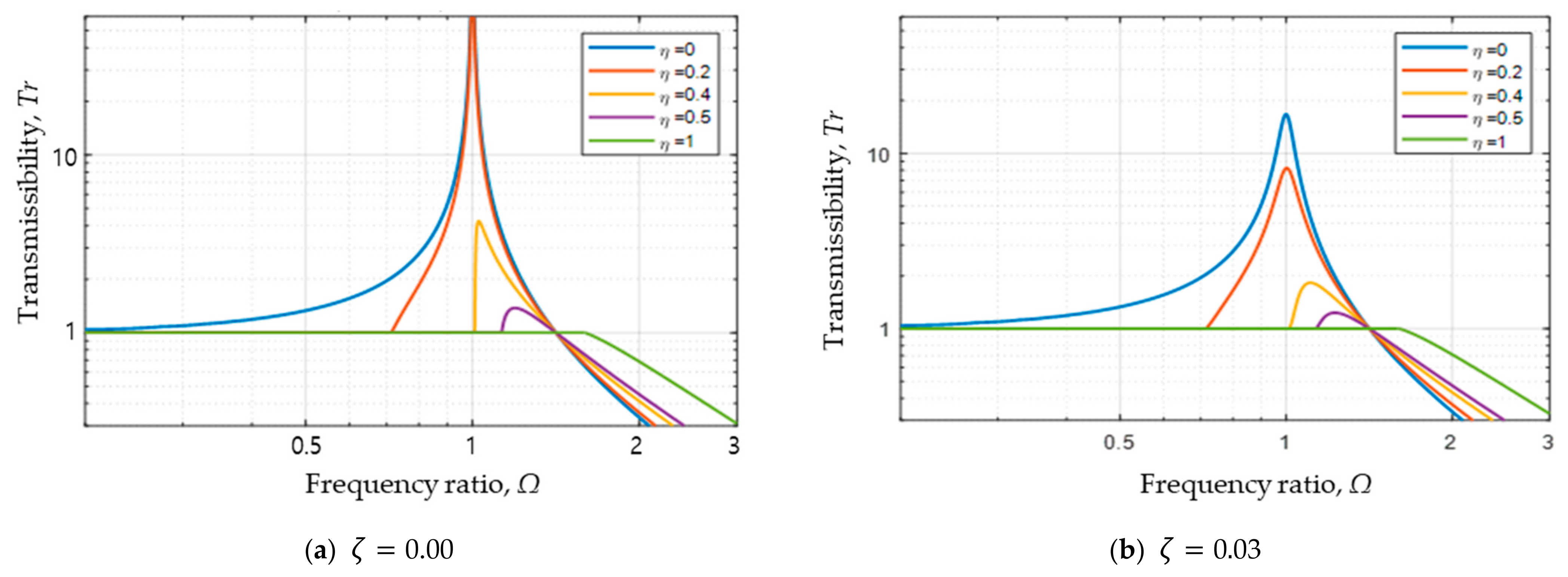
4.1. System with Zero Nonlinear Spring Coefficient ($\mu =0)$

In the case where the coefficient of nonlinear stiffness ${\mathrm{k}}_3$ in the equation of motion Equation (1) is zero, the DTR can be obtained by numerical analysis, and the result can be obtained, as shown in Figure 3. As shown in Figure 3a,b, as the excitation frequency ratio increases, the frequency at which DTR begins to become greater than one increases as the friction ratio $\eta$ increases. This is because the break-loose frequency increases as the friction ratio increases, so there is no relative motion until the excitation frequency reaches the break-loose frequency, maintaining $T_r=1$. Also, all DTR curves always pass the point of $T_r=1$ when $\Omega =\sqrt{2}$. Since this is a case that satisfies $u_s=-2\mathit{cos}{\varphi }_s$ in Equation (18), by substituting this into Equation (11), confirms that $\Omega =\sqrt{2}$. When $\eta <\mathsf{\pi }/8$ (${\Omega }_c<1$), resonance occurs at $\Omega =1$. For instance, as shown in Figure 3a, when $\eta =0$ or $\eta =0.2$ ($\eta <\mathsf{\pi }/8$) with $\zeta =0$, the DTR becomes infinite at $\Omega =1$ in both cases. However, in Figure 3b, where $\zeta \ne 0$, the DTR is finite due to the effect of viscous damping. When $\eta >\mathsf{\pi }/8$ (${\Omega }_c>1$), the DTR rapidly decreases, and when $\eta \ge \mathsf{\pi }/4$ (${\Omega }_c\ge \sqrt{2}$), the DTR becomes less than or equal to one at all excitation frequencies ($\Omega \ge \sqrt{2})$, resulting in vibration isolation.

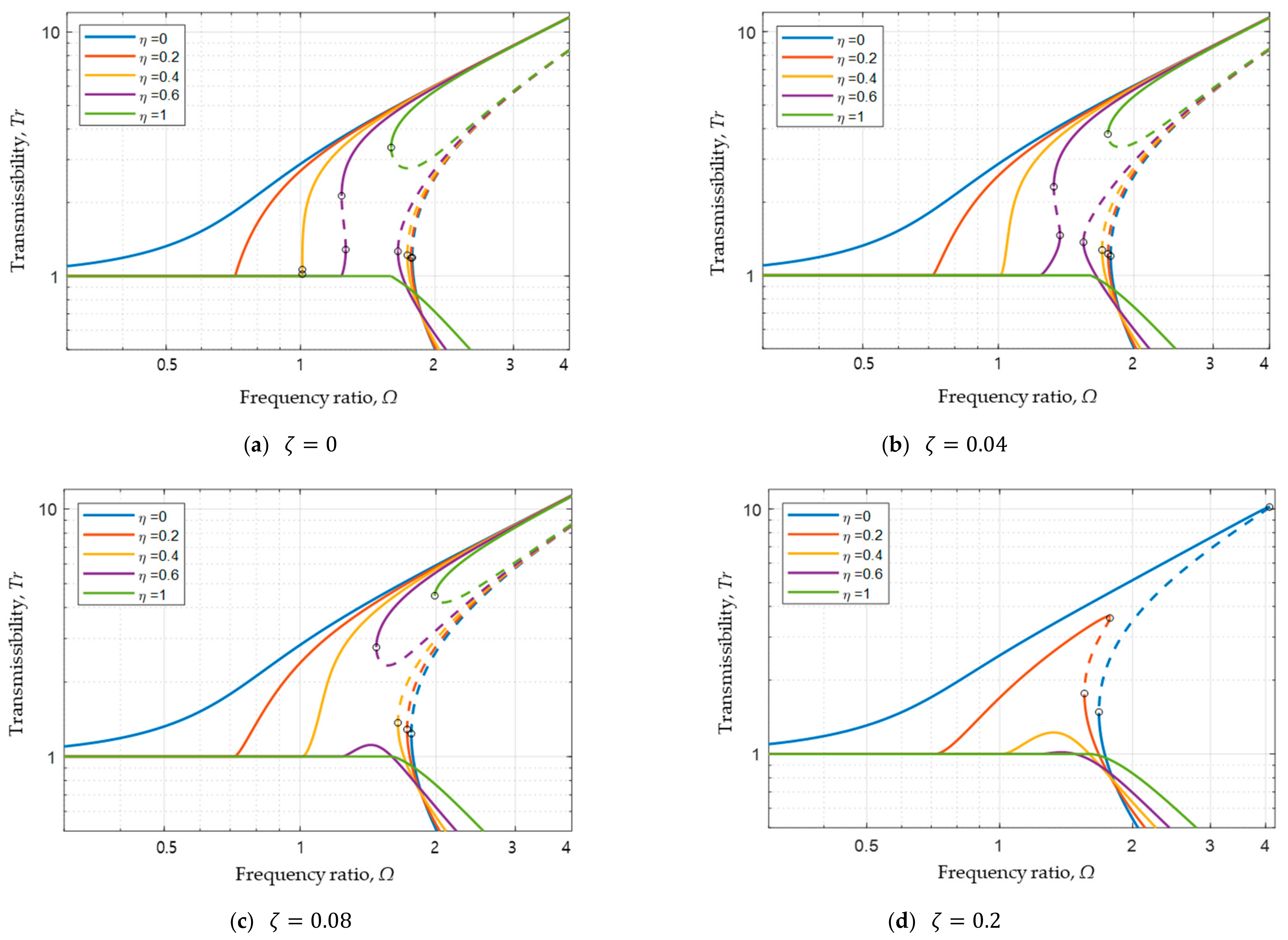
4.2. System with Positive Nonlinear Spring Coefficient ($\mu >0)$

For the system where the linear and nonlinear spring constants are non-zero, the TRs of the equation of motion (1) were numerically analyzed with respect to changes in the damping ratio $\zeta$ and friction ratio $\eta$. The results are shown in Figure 4. Depending on the frequency ratio, the system has either one or three solutions for the DTR. The stability of these solutions is evaluated using Equation (16), and unstable solutions are represented by dashed lines. A limit point (LP) bifurcation occurs when the system transitions from one solution to three, or from three solutions to one, and this LP bifurcation is marked with circular symbols. When the excitation frequency is lower than the break-loose frequency, no relative motion occurs due to the friction damper, and the DTR remains at one. As shown in Figure 4a, when the friction ratio $\eta$ increases, the break-loose frequency also increases. With a further increase in the break-loose frequency, the front resonant branch of the DTR curve bifurcates into one unstable solution and two stable solutions, forming a concave shape. As the values continue to rise, the front resonant branch and rear resonant branch meet at a single point, indicating that the solution possesses multiple roots. Subsequently, the DTR curve separates into a host branch and a sub-branch. The results of this numerical analysis are presented in Figure 4. In Figure 4a–c, examining the cases where $\eta$ is 0.6 and 1, it can be seen that as the damping ratio $\zeta$ increases, the separation of the DTR curve also occurs. From the perspective of the damping ratio, considering $\eta =0.6$, it is noted that as $\zeta$ increases to 0, 0.04, and 0.06, the DTR curve separates into the host branch and sub-branch. In Figure 4d, when the damping ratio is large (e.g., $\zeta =0.2$), it is noted that even as the friction ratio increases, the front resonant branch maintains stable solutions without bifurcation, while the rear resonant branch shows bifurcation or stable solutions depending on the value of the damping ratio.

In the analysis of Figure 4, DTR can be classified into three types based on the system design parameters, as shown in Figure 5. These types include Type I, where the front resonant branch of the DTR curve undergoes bifurcation; Type II, where the TR curve separates into a host branch and a sub-branch; and Type III, where there is no bifurcation in the front resonant branch of the DTR curve.

Type I, illustrated in Figure 5a, features a concave or narrow-waist shape due to the LP bifurcation points A and B, where the corresponding frequencies satisfy ${\Omega }_A>{\Omega }_B$. This type also exhibits abnormal jump characteristics. When the excitation frequency is swept upward from point S, it follows the S-A path and jumps up at point A, moving along the upper resonant branch to point E. Conversely, when sweeping the frequency downward from point F, it follows the F-C path, jumps up at point C, and subsequently moves along the upper resonant branch to point B before jumping down and reaching point S. This results in a double jump phenomenon.

Type II, depicted in Figure 5b, exhibits DTR characteristics that are separated into a host branch and a sub-branch. In the case of a downward sweep from point E of the sub-branch, a jump down occurs at point D along the upper sub-branch, although this is a very specific scenario and has a low probability of occurrence in practical engineering. Upward or downward sweeps from points S or F lie on the stable host branch along the S-F path. However, the separated sub-branch has a large transmissibility characteristic, and due to its distinct properties, it may not be identified in analyses using the shooting method [43]. Therefore, caution should be exercised during the analysis.

Type III, shown in Figure 5c, is characterized by the absence of bifurcation in the front resonant branch of the DTR curve. If the viscous damping is significant, the rear resonant branch also exhibits stable solutions.

Consequently, it is essential to investigate the relationships among the design parameters: the damping ratio $\zeta$, the friction ratio $\eta$, and the coefficient of cubic nonlinearity $\mu$, as bifurcation phenomena related to instability arise based on these relationships. Understanding these relationships is critical for the vibration isolation design of nonlinear systems.

The LP bifurcations of the DTR curves vary according to the design parameters: friction ratio, damping ratio, and coefficient of cubic nonlinearity. By tracking the changes in these bifurcations, one can understand the characteristics of the DTR curve. First, fixing $\zeta =0.02$ and $\eta =0.2$, and calculating the bifurcation points of the DTR curves for several friction ratio values, the results shown in Figure 6a are obtained. In this figure, points A and C merge into point D ($\eta =0.6565$) as $\eta$ increases. Beyond this point, the bifurcations disappear. Meanwhile, point B follows a path from point E to point F as $\eta$ increases. Figure 6b shows the trajectory of the bifurcation points in the $\Omega -\eta$ plane, obtained by incrementally changing the friction ratio $\eta$. The points corresponding to the bifurcations in Figure 6a are marked with the same labels in Figure 6b. The kink point on the trajectory curve is labeled as $K_p$, the intersection with the horizontal line is labeled as $R_p$, and the critical point is denoted as $C_p$. As seen in Figure 6b, bifurcation points A and C move closer together as η increases and eventually converge at the critical point $C_p$, which corresponds to point D ($\eta ={\eta }_D$). Conversely, as $\eta$ decreases, bifurcation points B and A approach each other, forming a kink point $K_p$, and the unstable region disappears.

Thus, when ${\eta }_{K_p}<\eta <{\eta }_{C_p}$, the DTR curve exhibits a Type I form with two bifurcations, leading to unstable solutions on the front resonant branch. When $\eta >{\eta }_{C_p}$, the DTR curve separates into a host branch and a sub-branch with one bifurcation, forming a Type II shape. Finally, when ${\eta <\eta }_{K_p}$, the DTR curve has no unstable solutions on the front resonant branch, resulting in a Type III shape. Consequently, by using the trajectory curve as shown in Figure 6b, the frequency response characteristics can be effectively identified according to the variation in $\eta$.

The following analyzes the changes in bifurcation points with respect to the damping ratio $\zeta$. DTR curves for various $\zeta$ values were calculated, and the bifurcation points of each DTR curve were tracked and plotted on the $\Omega -\eta$ plane, as shown in Figure 7. First, for $\zeta$ = 0, the kink point $K_p$ is located at the coordinates ($\Omega$, η) = (1, 0.393) on the boundary line between stick and slip, which can be verified by the break-loose frequency relation (15). The critical point $C_p$ is located at the coordinates (1.492, 0.695). As $\zeta$ increases to 0.02 and 0.08, the range of friction ratios between $K_p$ and $C_p$ on the trajectory curve, i.e., from ${\eta }_{K_p}$ to ${\eta }_{C_p}$, decreases. Consequently, as viscous damping increases, the range of friction ratios for which the DTR curve takes the form of Type I diminishes. Additionally, since the friction ratio at the critical point $C_p$, ${\eta }_{C_p}$, decreases, the range of friction ratios forming the Type II curve increases. When $\zeta$ = 0.15, $C_p$ and $R_p$ disappear, leaving only $K_p$. At this point, $K_p$ is located at the coordinates (1.4417, 0.3835). If $\eta >{\eta }_{K_p}=0.3835$, the DTR curve exhibits Type II characteristics, and if $\eta <{\eta }_{K_p}$, it exhibits Type III characteristics. Similarly, when $\zeta$ = 0.2, only $K_p$ exists at the coordinates (1.4977, 0.2405), and since η is always less than ${\eta }_{K_p}$, the DTR curve shows Type III characteristics.

By tracking the changes in the bifurcation points $C_p$, $K_p$, and $R_p$ along the bifurcation path in Figure 7 and reconstructing them on the $\zeta -\eta$ plane using their $\zeta$ and η values, the tracking diagram shown in Figure 8 is obtained. In Figure 8, the $R_p$ line partially overlaps with the $K_p$ line, and the $C_p$ line decreases as $\zeta$ increases, eventually merging with the $K_p$ and $R_p$ lines and vanishing at $\zeta$ ≃ 0.13. These two lines divide the $\zeta -\eta$ plane into three regions. Analyzing the DTR curve characteristics in the three regions of Figure 8, in Zone I, where ${\eta }_{K_p}<\eta <{\eta }_{C_p}$, the DTR curve exhibits Type I characteristics with bifurcations in both the front and rear resonant branches. Zone III, where $\eta <{\eta }_{K_p}$ shows no bifurcation in the front resonant branch but bifurcation in the rear resonant branch, displaying Type II and Type III characteristics. In Zone II, where $\eta >{\eta }_{C_p}$ and $\eta >{\eta }_{K_p}$, the DTR curve splits into host and sub-branches, with the host branch having no bifurcation, corresponding to Type II and Type III characteristics. Zone II can be considered a parameter region where the system’s response is stable.

The tracking diagram in Figure 8, obtained by tracing significant points such as $K_p$ and $C_p$ along the bifurcation curves, provides valuable information for selecting design parameters, η and ζ, to stabilize the system, offering highly useful guidance for the design process.

The following analyzes the system’s response characteristics with changes in the value of the coefficient of cubic nonlinearity $\mu$, presenting the tracking diagram of $C_p$ and $K_p$ at $\mu =0.5$ in Figure 9. As seen in Figure 9, this diagram resembles Figure 8 but shows enlarged Zone I and Zone III. Notably, as the nonlinear stiffness increases, Zone I expands, which requires careful consideration when selecting the design parameters for the system. Figure 10 illustrates the effects of the nonlinear stiffness coefficient by adding cases for $\mu$ = 0.5 and 1, represented in a three-dimensional $\zeta -\eta -\mu$ space. As shown in Figure 10, it consists of three distinct spatial regions, and the DTR characteristics in each region are extensions of the results already discussed in Figure 8. Therefore, the results of Figure 10 can be used as useful material for setting the design parameters for vibration isolation, namely, the friction ratio, damping ratio, and the coefficient of cubic nonlinearity, according to specific objectives.

5. Conclusions

The response characteristics of the nonlinear isolation system with friction damping, viscous damping, and nonlinear stiffness, attributed to the base excitation, were analyzed using the SVAP method, and the results are as follows.

The break-loose frequency where the relative motion of the system occurs can be predicted by deriving the functional relationship of the friction damping ratio. In a nonlinear system with friction damping, the break-loose frequency increases as the friction coefficient increases, and the bifurcation phenomenon of the solution occurs in the front resonant branch. On the other hand, when the friction and viscous damping ratio increases, the bifurcation phenomenon of the solution disappears in the front resonant branch, and the bifurcation of the solution also disappears in the rear resonant branch. These phenomena can be classified into three types. The three types include configurations where unstable points (saddle points) exist in certain intervals of the DTR curve due to variations in design parameters, configurations with separated shapes of the DTR curve, and configurations where no separation phenomenon occurs. By tracking the bifurcation and its trajectory with respect to the design parameters, and following the key points $K_p$ and ${\mathrm{C}}_p$, the system’s parameter space could be divided into three zones on the $\eta -\zeta$ plane, allowing the specific type of DTR curve in each zone to be identified. Furthermore, by incorporating the nonlinear stiffness $\mu$, the analysis was extended into a three-dimensional space of $\zeta$, $\eta$, and $\mu$, confirming that as $\mu$ increases, the number of unstable regions also increases. The presentation of the three-dimensional space can serve as a valuable resource for easily determining stability and can be utilized for selecting design parameters. In other words, this is expected to serve as a resource for analyzing and selecting the interrelationships of design parameters such as the friction ratio $\eta$, damping ratio $\zeta$, and nonlinear stiffness coefficient $\mu$, which are key design variables in vibration isolation systems to ensure stability. Furthermore, by presenting a methodology for analyzing the response characteristics using the SVAP method, it is anticipated that this approach can be widely applied to single-degree-of-freedom nonlinear vibration isolation systems with friction and 1st- and 3rd-order nonlinear springs. Future research may explore additional nonlinear effects or integrate different damping mechanisms to expand upon this study.

References

1. Liu, C.; Jing, X.; Daley, S.; Li, F. Recent advances in micro-vibration isolation. Mech. Syst. Signal Process. 2015, 56–57, 55–80. [Google Scholar] [CrossRef]
2. Yan, B.; Yu, N.; Wu, C. A state-of-the-art review on low-frequency nonlinear vibration isolation with electromagnetic mechanisms. Appl. Math. Mech.-Engl. 2022, 43, 1045–1062. [Google Scholar] [CrossRef]
3. Santhosh, B.; Narayanan, S.; Padmanabhan, C. Nonlinear Dynamics of Shrouded Turbine Blade System with Impact and Friction. Appl. Mech. Mater. 2014, 76, 81–92. [Google Scholar] [CrossRef]
4. Le, T.D.; Ahn, K.K. A vibration isolation system in low frequency excitation region using negative stiffness structure for vehicle seat. J. Sound Vib. 2011, 330, 6311–6335. [Google Scholar] [CrossRef]
5. Le, T.D.; Ahn, K.K. Experimental investigation of a vibration isolation system using negative stiffness structure. Int. J. Mech. Sci. 2013, 70, 99–112. [Google Scholar] [CrossRef]
6. Lang, Z.Q.; Jing, X.J.; Billings, S.A.; Tomlinson, G.R.; Peng, Z.K. Theoretical study of the effects of nonlinear viscous damping on vibration isolation of sdof systems. J. Sound Vib. 2009, 323, 352–365. [Google Scholar] [CrossRef]
7. Yuvaraju, B.A.G.; Srinivas, J.; Nanda, B.K. Nonlinear dynamics of friction-induced regenerative chatter in internal turning with process damping forces. J. Sound Vib. 2023, 544, 117386. [Google Scholar] [CrossRef]
8. Ruzicka, J.E.; Derby, T.F. Influence of Damping in Vibration Isolation, SVM-7; Shock and Vibration Information Center: Washington DC, USA, 1971. [Google Scholar]
9. Ibrahim, R.A. Recent advances in nonlinear passive vibration isolators. J. Sound Vib. 2008, 314, 371–452. [Google Scholar] [CrossRef]
10. Ledezma-Ramírez, D.F.; Tapia-González, P.E.; Ferguson, N.; Brennan, M.; Tang, B. Recent advances in shock vibration isolation: An overview and future possibilities. Appl. Mech. Rev. 2019, 71, 060802. [Google Scholar] [CrossRef]
11. Rivin, E.I. Passive Vibration Isolation; ASME Press: New York, NY, USA, 2003. [Google Scholar]
12. Hong, S.C.; Hur, D.J. Dynamic behavior of a simple rolling seismic isolator with a position restoring device. Appl. Sci. 2018, 8, 1910. [Google Scholar] [CrossRef]
13. Hur, D.J.; Hong, S.C. Analysis of an isolation system with vertical spring-viscous dampers in horizontal and vertical ground motion. Appl. Sci. 2020, 10, 1141. [Google Scholar] [CrossRef]
14. Shin, Y.H.; Lee, J.H.; Jung, B.C.; Moon, S.J. Design of passive vibration isolation element by wire mesh material for developing a hybrid mount. Trans. Korean Soc. Noise Vib. Eng. 2020, 30, 75–81. [Google Scholar] [CrossRef]
15. Alrajhi, J.; Alhaifi, K.; Alardhi, M.; Alhaifi, N.; Alazmi, J.; Khalfan, A.; Alkhulaifi, K. The numerical analysis of single degree of freedom vibration system with non-linearity. J. Mech. Eng. Autom. 2023, 12, 6–19. [Google Scholar]
16. Min, K.W.; Kim, H.S. Performance based design of friction dampers for seismically excited structures. J. Earthq. Eng. Soc. Korea 2003, 7, 17–24. [Google Scholar]
17. Krack, M.; Gross, J. Harmonic Balance for Nonlinear Vibration Problems; Springer Nature: Cham, Switzerland, 2019. [Google Scholar]
18. Mickens, R.E. Truly Nonlinear Oscillations, Harmonic Balance, Parameter Expansions, Iteration, and Averaging Methods; World Scientific Publishing Company: Danvers, MA, USA, 2010. [Google Scholar]
19. Hagedorn, P. Non-Linear Oscillations; Clarendon Press: Oxford, UK, 1981. [Google Scholar]
20. Sanders, J.A.; Verhulst, F.; Murdock, J. Averaging Methods in Nonlinear Dynamical Systems, 2nd ed.; Springer: New York, NY, USA, 2007. [Google Scholar]
21. Nayfeh, A.H.; Mook, D.T. Nonlinear Oscillations; John Wiley & Sons: Hoboken, NJ, USA, 1995. [Google Scholar]
22. Shahraeeni, M.; Sorokin, V.; Mace, B.; Ilanko, S. Effect of damping nonlinearity on the dynamics and performance of a quasi-zero-stiffness vibration isolator. J. Sound Vib. 2022, 526, 116822. [Google Scholar] [CrossRef]
23. Ma, Z.; Zhou, R.; Yang, Q. Recent advances in quasi-zero stiffness vibration isolation systems: An overview and future possibilities. Machines 2022, 10, 813. [Google Scholar] [CrossRef]
24. Brennan, M.J.; Kovacic, I.; Carrella, A.; Waters, T.P. On the jump-up and jump-down frequencies of the Duffing oscillator. J. Sound Vib. 2008, 318, 1250–1261. [Google Scholar] [CrossRef]
25. Carrella, A.; Brennan, M.J.; Waters, T.P.; Lopes, V. Force and displacement transmissibility of a nonlinear isolator with high-static-low-dynamic-stiffness. Int. J. Mech. Sci. 2012, 55, 22–29. [Google Scholar] [CrossRef]
26. Barquist, C.S.; Jiang, W.G.; Gunther, K.; Lee, Y. Determining the source of phase noise: Response of a driven Duffing oscillator to low-frequency damping and resonance frequency fluctuations. Phys. D Nonlinear Phenom. 2021, 427, 13299. [Google Scholar] [CrossRef]
27. Liu, S.; Peng, G.; Li, Z.; Li, W. Analytical jump-avoidance criteria of Duffing-type vibration isolation systems under base and force excitations based on concave-convex property. J. Vib. Control 2023, 29, 4082–4092. [Google Scholar] [CrossRef]
28. Murata, A.; Kume, Y.; Hashimoto, F. Application of catastrophe theory to forced vibration of a diaphragm air spring. J. Sound Vib. 1987, 112, 31–44. [Google Scholar] [CrossRef]
29. Kovacic, I.; Brennan, M.J.; Lineton, B. On the resonance response of an asymmetric Duffing oscillator. Int. J. Non-Linear Mech. 2008, 43, 858–867. [Google Scholar] [CrossRef]
30. Shi, B.; Yang, J.; Li, T. Enhancing Vibration Isolation Performance by Exploiting Novel Spring-Bar Mechanism. Appl. Sci. 2021, 11, 8852. [Google Scholar] [CrossRef]
31. Marino, L.; Cicirello, A.; Hills, D.A. Displacement transmissibility of a Coulomb friction oscillator subject to jointed base-wall motion. Nonlinear Dyn. 2019, 98, 2595–2612. [Google Scholar] [CrossRef]
32. Wang, D.; Song, L.; Zhu, R.; Cao, P. Nonlinear dynamics and stability analysis of dry friction damper for supercritical transmission shaft. Nonlinear Dyn. 2022, 110, 3135–3149. [Google Scholar] [CrossRef]
33. Uzdin, A.M.; Kuznetsova, I.O.; Frese, M.; Nazarova, S.S.; Nazarov, A.A. Analysis of the behaviour of seismic isolated structure on bearings connected to the structure with a dry friction damper. AIP Conf. Proc. 2023, 2612, 040012. [Google Scholar]
34. Benacchio, S.; Giraud-Audine, C.; Thomas, O. Effect of dry friction on a parametric nonlinear oscillator. Nonlinear Dyn. 2022, 108, 1005–1026. [Google Scholar] [CrossRef]
35. Zucca, S.; Firrone, C.M. Nonlinear dynamics of mechanical systems with friction contacts: Coupled static and dynamic multi-harmonic balance method and multiple solutions. J. Sound Vib. 2014, 333, 916–926. [Google Scholar] [CrossRef]
36. Ferhatoglu, E.; Zucca, S. Determination of periodic response limits among multiple solutions for mechanical systems with wedge dampers. J. Sound Vib. 2021, 494, 115900. [Google Scholar] [CrossRef]
37. Ferhatoglu, E.; Groß, J.; Krack, M. Frequency response variability in friction-damped structures due to non-unique residual tractions: Obtaining conservative bounds using a nonlinear-mode-based approach. Mech. Syst. Signal Process. 2013, 201, 110651. [Google Scholar] [CrossRef]
38. Starossek, U. Exact analytical solutions for forced cubic restoring force oscillator. Nonlinear Dyn. 2016, 83, 2349–2359. [Google Scholar] [CrossRef]
39. Ravindra, B.; Mallik, A.K. Hard Duffing-type Vibration Isolator with Combined Coulomb and Viscous Damping. Int. J. Non-Linear Mech. 1993, 28, 427–440. [Google Scholar] [CrossRef]
40. Yu, H.; Zhang, L. Free resonance analysis of bilinear hysteresis dry friction damper. J. Vib. Shock 2016, 3, 92–95. [Google Scholar]
41. Huang, X.; Sun, J.; Hua, H.; Zhang, Z. The isolation performance of vibration systems with general velocity-displacement-dependent nonlinear damping under base excitation: Numerical and experimental study. Nonlinear Dyn. 2016, 85, 777–796. [Google Scholar] [CrossRef]
42. Yu, H.; Xu, Y.; Sun, X. Analysis of the non-resonance of nonlinear vibration isolation system with dry friction. J. Mech. Sci. Technol. 2018, 32, 1489–1497. [Google Scholar] [CrossRef]
43. Dhooge, A.; Govaerts, W.; Kuznetsov, Y.A. MATCONT: A Matlab Package for Numerical Bifurcation Analysis of ODEs. ACM Trans. Math. Softw. 2003, 29, 141–164. [Google Scholar] [CrossRef]
Figure 1. Base excited nonlinear vibration system including friction damping.
Vibration 07 00062 g001
Figure 2. Sticking and slip regions in Ω η plane and the separating threshold line.
Vibration 07 00062 g002
Figure 3. Absolute displacement transmissibility of linear spring system ( μ = 0 ). (a) Transmissibility curve due to frequency ratio at ζ = 0.00 for η = 0, 0.2, 0.4, 0.5, 1.0, (b) Transmissibility curve due to frequency ratio at ζ = 0.03 for η = 0, 0.2, 0.4, 0.5, 1.0.
Vibration 07 00062 g003
Figure 4. Absolute displacement transmissibility of a nonlinear system with respect to friction and frequency ratio for a spring stiffness ratio of μ = 0.2. The dashed lines denote the unstable branch regions, and the circle markers indicate the locations of the LP bifurcations. (a) Transmissibility curve due to frequency ratio at ζ = 0.00, (b) Transmissibility curve due to frequency ratio at ζ = 0.04, (c) Transmissibility curve due to frequency ratio at ζ = 0.08, (d) Transmissibility curve due to frequency ratio at ζ = 0.2 for η = 0, 0.2, 0.4, 0.6, 1.0.
Vibration 07 00062 g004
Figure 5. Three types of displacement transmissibility responses that occur depending on system design parameters; the dotted line is an unstable region; and the end point of the dotted line is the LP Bifurcation point. (a) Type I with a concave or narrow-waist shape due to the LP bifurcation points ( ζ = 0.02 ,   μ = 0.2 ,   η = 0.6 ), (b) Type II separated into a host branch and a sub-branch ( ζ = 0.08 ,   μ = 0.2 ,   η = 0.6 ), (c) Type III without bifurcation in front resonant branch curve ( ζ = 0.2 ,   μ = 0.2 ,   η = 0.2 ).
Vibration 07 00062 g005aVibration 07 00062 g005b
Figure 6. Transition of TR curves and the trajectory of LP bifurcations in the Ω η plane, with μ = 0.2 and ζ = 0.02 . (a) Transmissibility curve due to frequency ratio for η = 0.7, 0.6565, 0.6, 0.5, 0.4, 0.5, 1.0 and Limit Point, (b) Trajectory of Limit Points due to friction ratio at the left figure.
Vibration 07 00062 g006
Figure 7. Trajectories of LP Bifurcations according to various damping ratios ζ for μ = 0.2 in the Ω η plane. The dashed line means the boundary between stick and slip.
Vibration 07 00062 g007
Figure 8. Tracking diagram of C p , K p , and R p points in ζ η plane with μ = 0.2 and regions delineated by them. (Sky blue is zone I, white is zone II, coral is zone III).
Vibration 07 00062 g008
Figure 9. Tracking diagram of C p and K p points in ζ η plane with μ = 0.5 and regions delineated by them. (Sky blue is zone I, white is zone II, coral is zone III).
Vibration 07 00062 g009
Figure 10. Tracking diagram of C p and K p points in ζ μ η space and regions delineated by them. (Zone I is a volume where the sky blue colored areas are connected in the nonlinear stiffness ratio μ direction, zone II is a volume where the white-colored areas are connected, and zone III is a volume where the coral-colored areas are connected).
Vibration 07 00062 g010
Disclaimer/Publisher’s Note: The statements, opinions and data contained in all publications are solely those of the individual author(s) and contributor(s) and not of MDPI and/or the editor(s). MDPI and/or the editor(s) disclaim responsibility for any injury to people or property resulting from any ideas, methods, instructions or products referred to in the content.