2.1. Data Collection
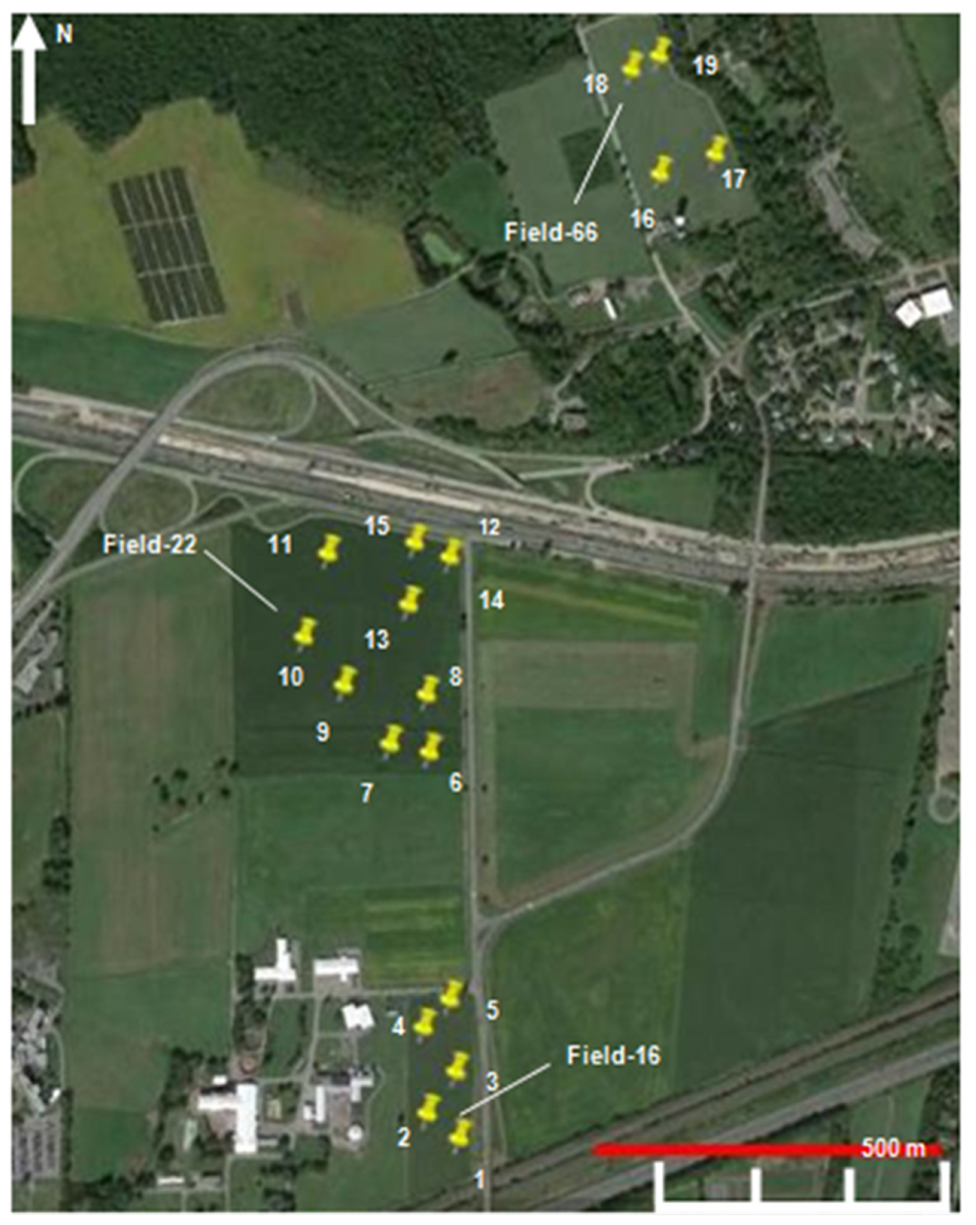
Three fields at McGill University Macdonald research farm (45°24′42.2″ N 73°56′23.1″ W; Sainte-Anne-de-Bellevue, QC, Canada) were used for this project. In total, nineteen locations were selected in these fields (
Figure 2) to represent diverse soil conditions ranging from sand to clay loam. The fields had 2.5, 4.5 and 12 ha areas and crops were grown according to a rotation involving soybean, corn (grain and silage) and alfalfa. All data were collected in 2012 when an alfalfa/grass mix was grown in each of the three fields.
In each location, composite soil samples were obtained from the top (0–20 cm) layer of soil. A 4 cm diameter, stainless steel auger was used to take five samples from within a 0.5 m radius. These soil cores were mixed, air dried, and sieved through a 2 mm mesh. Then, each sample was divided into two subsamples: one to be used for conventional laboratory analysis and the other for ex situ vis–NIR spectral measurements.
Three categories have been established for soil particles: sand, silt, and clay [
55]. These three groups are called soil separates. The three groups are divided by their particle size. Clay particles are the smallest, while sand particles are the largest. Particle size analysis (fractions of sand, silt, and clay) as well as SOM content were evaluated for each laboratory sample, as summarized in
Table 1. The particle size analysis was conducted using hydrometers [
1] and SOM was determined using the loss-on-ignition technique [
2].
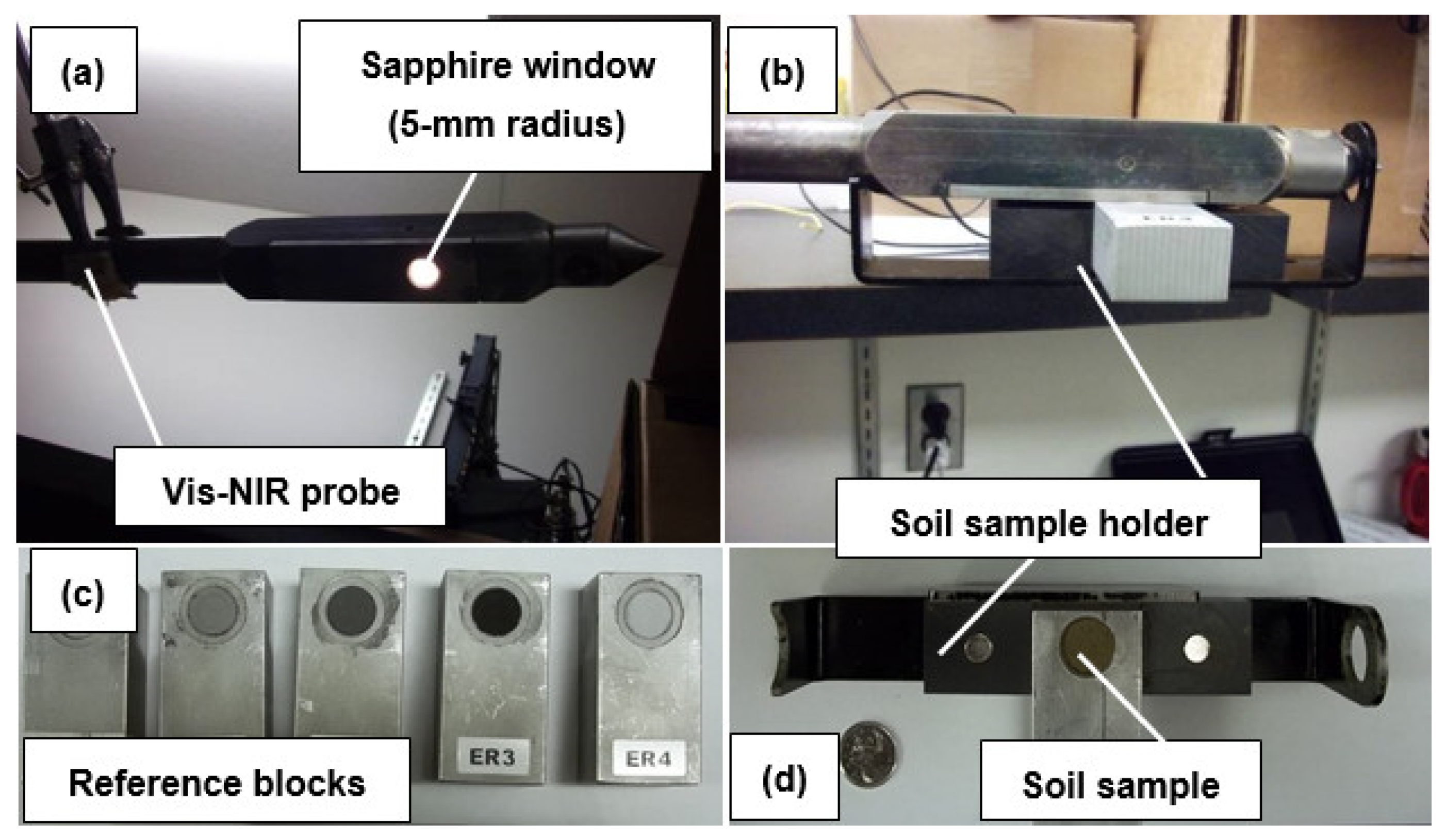
The core of the Veris P4000 instrument is a combined dual type spectrophotometer operating in the visible and near-infrared parts of the electromagnetic spectra (
Figure 3). One of the two spectrophotometers was USB2000 (Ocean Optics, Dunedin, FL, USA) operating between 342 and 1023 nm with a spectral resolution of 6 nm. The other spectrophotometer was C9914GB (Hammatsu Photonics. K.K., Tokyo, Japan), which collected data between 1070 and 2220 nm with a spectral resolution of 4 nm. The instrument included its own light source and was capable of maintaining a constant distance between measured soil surfaces and detectors by means of a sapphire contact probe with fibre-optic cables.
All ex situ measurements were conducted as triplicates in a different randomised order for each replicate. A specially designed sample holder (
Figure 3b) was filled with <1 g of the soil sample and placed near the optical window of the soil profiling tool. As was recommended in the user manual provided by the manufacturer, at the beginning of each spectral measurement session, the instrument was calibrated by measuring the dark current followed by the white reference measurements using the specially provided reference blocks, as shown in
Figure 3c. The instrument was re-calibrated after every 20 samples. Soil spectra were interpolated to about 5 nm of the spectral resolution, yielding a total of 380 data points (wavelengths) per spectrum. To minimize the instrument noise, each spectrum was the average of 25–30 scans (~6 scans s
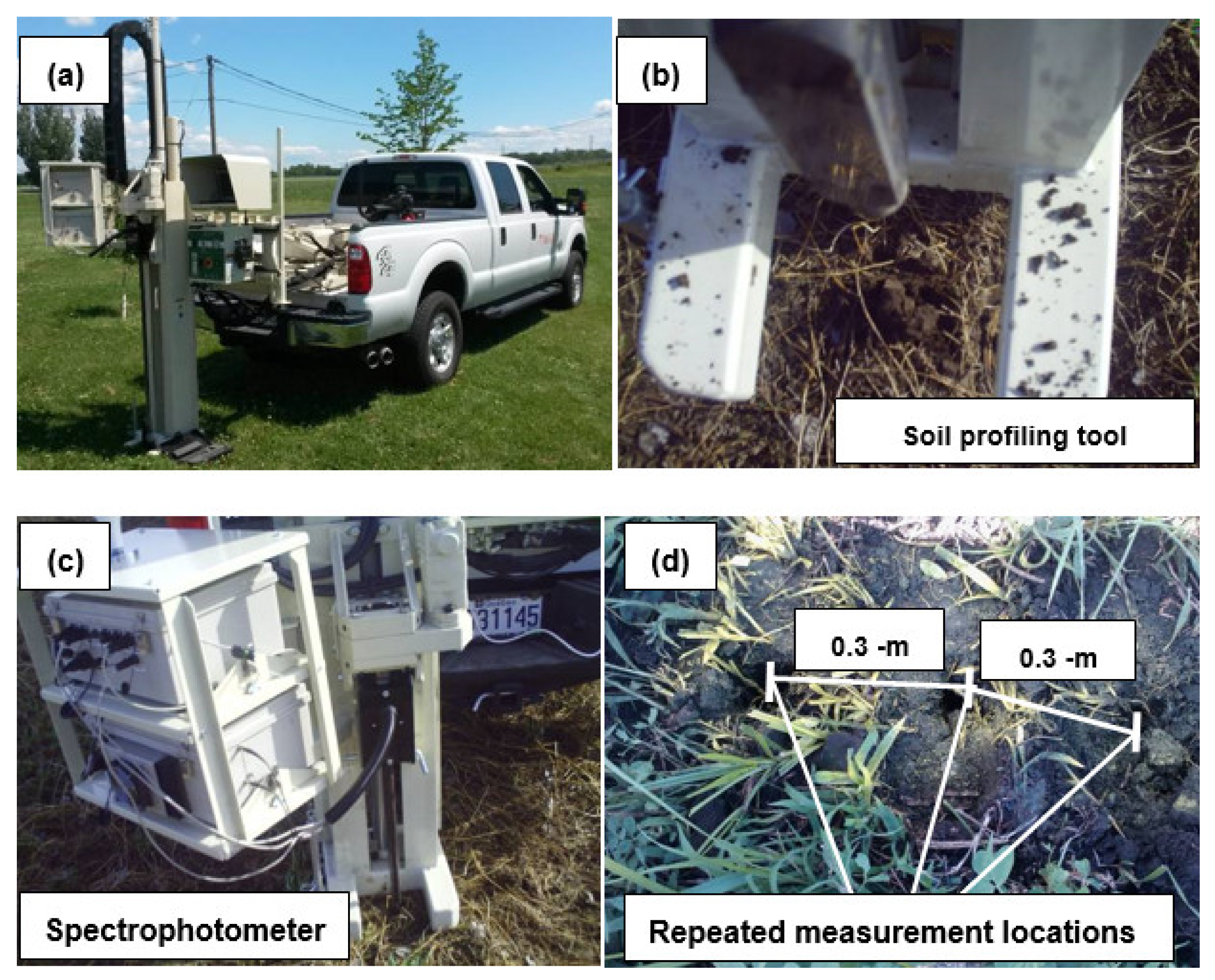
−1). The in situ measurements were collected using the recommended equipment setup (
Figure 4) for topsoil profiles down to 20 cm, while penetrating soil at a speed approximately 2 cm s
−1. Three measurements were conducted consecutively along a straight line that was less than 0.5 m long. The instrument was re-calibrated in a similar manner as discussed for the ex situ measurements. The soil spectra data collection procedures for in situ and ex situ measurements were the same. However, in this case, the average of 50–60 scans represented soil spectra collected at different depths from 0 to 20 cm.
2.2. Data Processing
As discussed previously (in
Section 2.1) and as shown in
Figure 5, the DRS measurements were collected in triplicate on representative soil samples using the soil profiling tool (ex situ and in situ), whereas the representative soil samples were analyzed in laboratories to obtain the standard measurements of the soil attributes of interest. Next, the DRS measurements were processed to create three more data sets (four in total: Raw, Smooth, 1st SGD, and 2nd SGD). Later, to understand the random fluctuation of soil spectra within the same samples and between different samples, the spread (SD
SA) and the root mean squared deviation (RMSD) were calculated on the DRS measurements for all four data sets. Simultaneously, the best SLR and PLSR models were fit on all four DRS measurement data sets against the known standard measurements of the soil attributes of interest. Finally, while focusing on the reproducibility of soil reflectance and its direct link with soil attributes, precision- and accuracy-related components such as the ratio of spread over error (RSE), measurement precision (MP), standard error of prediction (SEP), and coefficient of determination (R
2), respectively, were calculated. These are explained in greater detail later in the text.
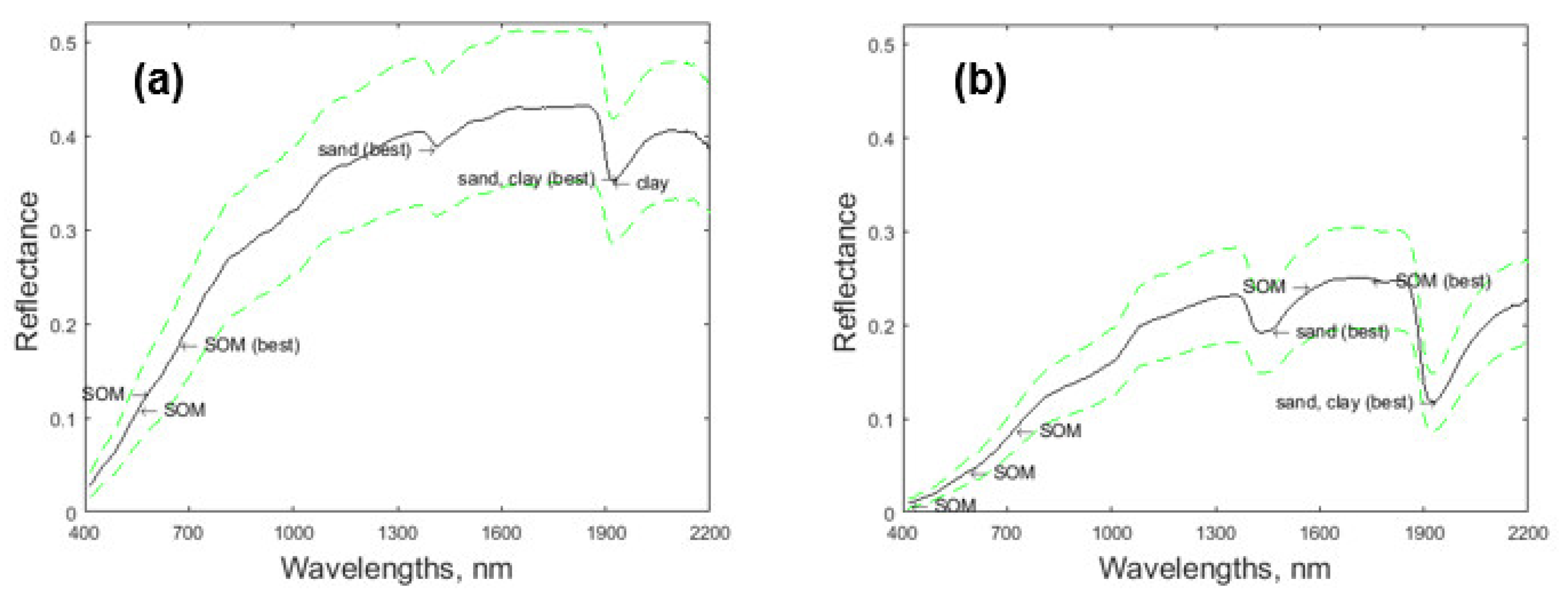
All raw spectral data were processed using MATLAB 2012a (The MathWorks, Inc. Natick, MA, USA) and ParLeS 3.1 software (University of Sydney, Sydney, Australia), as described by [
56]. All spectra exhibited a step discontinuity from 1023 to 1070 nm, caused by the transition from one detector to another. After removing the relatively noisy parts of the spectra at the edges of the detection ranges for each spectrophotometer (342–409 nm, 1014–1075 nm, and 2206–2220 nm), all resultant spectra consisted of a total of 363 measurements at different wavelengths. The spectral data were then corrected for offset and processed using a multiplicative scattering correction (MSC) algorithm [
57] and mean centering (MC). In addition to these “raw” spectra, the following spectra treatments were pursued: (1) 3-point Savitzky–Golay smoothing, (2) 11-point first order Savitzky–Golay derivative (1st SGD), and (3) 11-point second order Savitzky–Golay derivative (2nd SGD) [
58].
Among the different statistics considered for assessing the precision of spectral data, the RSE was used:
where
SDSA is the standard deviation of nineteen sample mean values;
RMSD is the root mean squared deviation calculated based on three replicated measurements for each of the nineteen samples.
where
= 19 is the number of soil samples;
is an average measured or calculated spectra related value for the
ith sample;
is the average of all
values.
where
= 3 is the number of replicated measurements;
is a
jth replicate of the measured or calculated spectra-related value for the
ith sample
Similar to the frequently used ratio of prediction over deviation (RPD) [
59], high RSE means a relatively strong ability of a given measurement to distinguish different soil samples. The use of RSE was reported earlier in [
60,
61] and is directly related to ANOVA F statistics used to compare the means of repeated measurements. Based on the degrees of freedom involved, the difference among the soil samples (means of three measurements) can be detected at α = 0.05 when RSE is greater than 0.79 (
). This analysis evaluates measurement precision with the underlying hypothesis that a particular parameter that does not change when measuring the same soil sample, and for which the change is at its maximum when measuring different samples, should be considered reliable.
The percentages of sand, clay, and SOM were predicted by fitting SLR models on each individual measured or treated spectral value versus these properties. A coefficient of determination (R
2) was the main indicator of the ability of a single spectral value to explain the variability in a particular soil property. However, the standard error of prediction (SEP) was used as a measure of the accuracy of soil property estimates obtained using each SLR model:
where
is the measured value of a given soil property for the
ith sample;
is the predicted value of a given soil property for the
ith sample and the
jth replicate;
(intercept) and
(slope) are coefficients of SLR.
where
y is the measured value of a given soil property for the
ith sample.
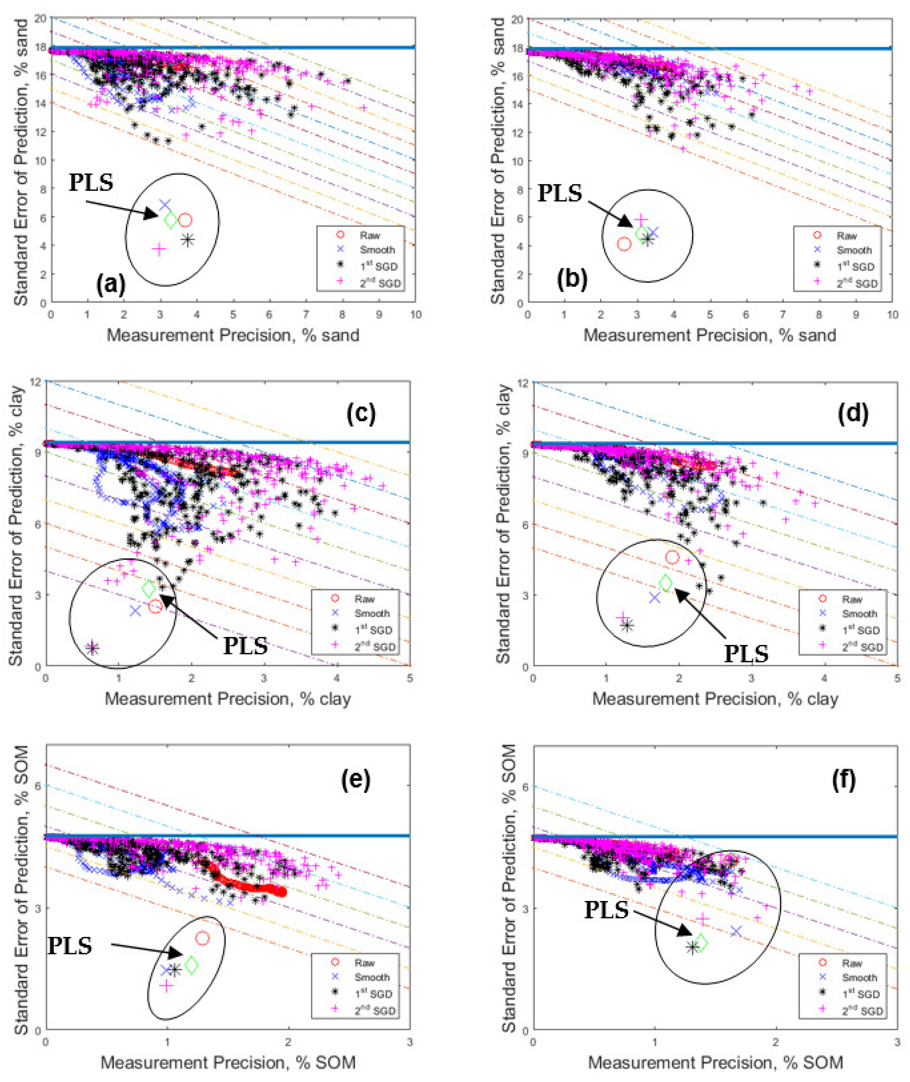
While SEP indicated the total error associated with each individual measurement and is primarily linked to the accuracy of prediction, RMSD is linked to measurement precision. However, since RMSD is expressed in the units of spectra measurements and related calculated parameters, measurement precision (MP) can be expressed in physical units as follows:
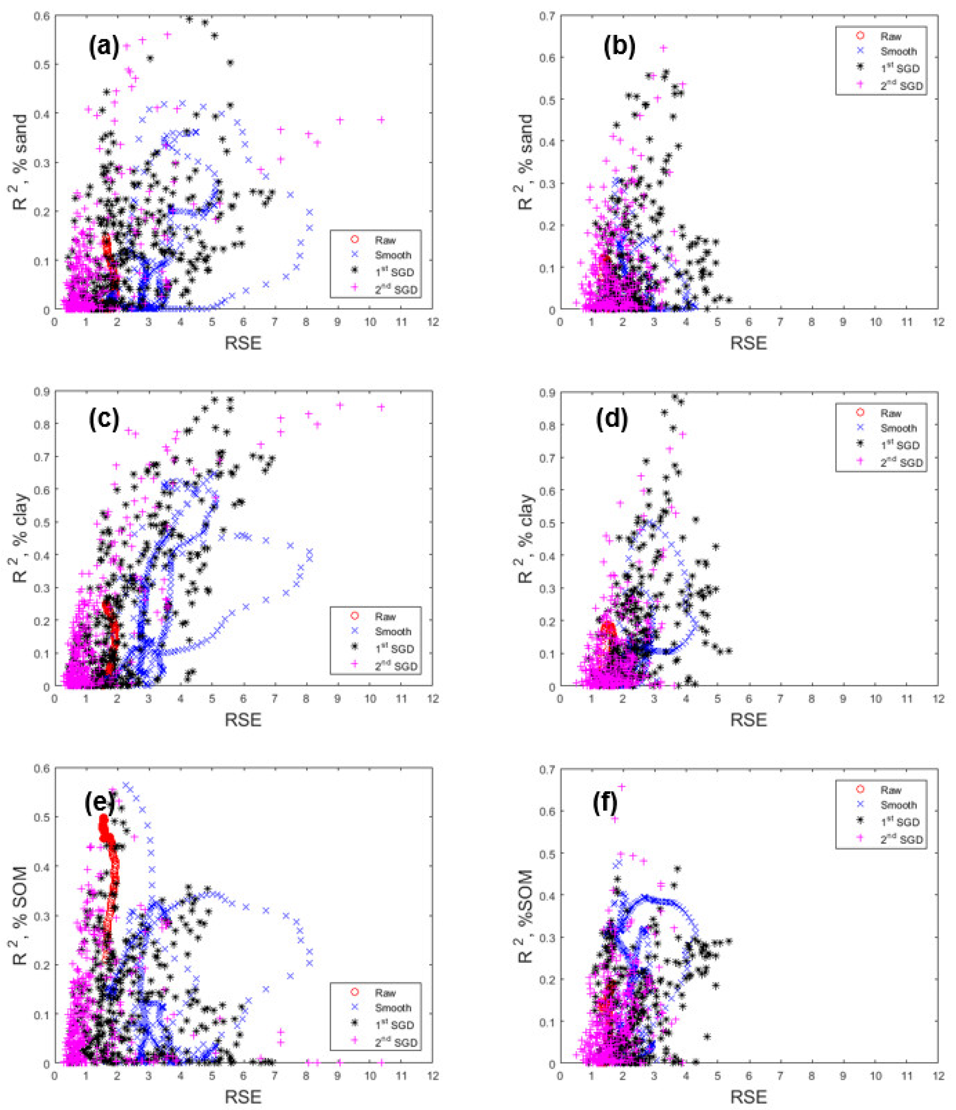
When comparing different spectral wavelengths and transformation techniques, it is important to identify measurements that have the maximum RSE and the minimum RMSD, MP, and SEP. The RMSD is an indicator of measurement reproducibility. However, without considering the spread of values across different samples, it is impossible to conclude if the given values are strong values to distinguish different soil samples from each other. Therefore, the RSE is involved in electing candidates to differentiate between the samples’ levels of disregard of the prediction property. Neither RMSD nor RSE depend on the model used to predict a given soil property.
Because of the SLR approach [
62] used to test one-input soil property prediction functions, RMSD can be expressed, in terms of the percentages of sand, clay, or SOM, as MP. The MP estimate is then evaluated together with SEP, which is the ultimate indicator of the predictability of soil properties. Unlike RMSD, the MP as well as the SEP can be compared across different spectra transformation procedures as both are expressed in physical units. From a sensor development point of view, a small RMSD and MP indicates a stable soil–detector interface. A high RSE means that the sensor can be applied to a particular set of soils. Finally, a small SEP (high R
2 for a given set of samples) indicates the sensor’s ability to predict the soil property of interest. The SEP is always greater than the MP, and the greater this difference, the less uncertain the linear relationship between the measured value and the property. Small differences between the SEP and MP indicate the applicability of the prediction model when reliable measurement estimates are obtained. In other words, small differences between the SEP and MP indicate the potential for improved predictability by averaging multiple unbiased measurements, but larger differences signify the limitations of the model and that alternative prediction methods, such as PLSR, should be involved.
In soil spectroscopy, PLSR is one of the most widely used techniques to aggregate measurements obtained at multiple wavelengths in a single prediction model [
32,
33,
34,
35] The PLSR is a bilinear regression technique that extracts a small number of latent factors, which are a combination of the independent variables, and uses these factors as a regression producer for the dependent variables [
63,
64]. The PLSR analysis is normally evaluated using the leave-one-out cross validation technique, and the RMSD, R
2 and Akaike Information Criterion (AIC), as described in [
65], are the most common model performance indicators.
In this study, the orthogonalised PLSR-1 algorithm described in [
66] was applied to (1) raw spectra, (2) smoothed spectra, (3) 1st SGD spectra, (4) 2nd SGD spectra, and (5) all the values were combined to develop calibration models using ParLeS software [
56]. The number of factors to use in each model was selected using leave-one-out cross validation. However, due to the limited number of soil samples used (
), the selected models were not re-validated on a different set of soil samples; however, this was generally undertaken in other reported studies. The developed models were used to estimate the performance indicators that were comparable to MP and SEP to define the superiority of PLSR over SLR models.


 ,
, 


