Abstract
The identification of iron (Fe) forms throughout a sediment sequence was investigated by X-ray Absorption Near Edge Spectroscopy (XANES) and Extended X-ray Absorption Fine Structure (EXAFS) at the Fe K-edge, paired with Raman micro-spectroscopy. The contribution of different organic and inorganic Fe-bearing compounds was quantified by Linear Combination Fitting (LCF) carried out on both XANES and EXAFS spectra. Fe-XANES showed that the Fe(II)/Fe(III) ratio of different Fe-bearing minerals in sediments can be quantified with reasonable accuracy. The main Fe species detected were ferrihydrite, goethite, hematite, clay minerals (smectite, illite, nontronite), and Fe(III)-organic matter (Fe(III)-OM). A more accurate quantification of ferrihydrite was possible with LCF conducted on Fe-EXAFS spectra. With the exception of hematite, the concentration of these mineral species does not have a clear trend with depth, probably because water infiltration caused continuous Fe reduction and oxidation cycles in these sediments. From an analytical perspective, Fe oxide compounds can be difficult to identify or distinguish unless multiple techniques are used. X-ray diffraction (XRD; previous work) and Raman spectroscopy turn out to be not particularly useful in identifying ferrihydrite, while they are best suited for a broad mineralogical analysis that requires integrative spectral studies for an accurate Fe speciation. In detail, XANES and EXAFS allowed for the detection of Fe-bearing clay minerals and a more refined identification of Fe species, including Fe(III)-OM. Thermal analysis was useful to confirm some mineralogical components observed using both XRD (data previously published) and Raman spectroscopy (e.g., goethite, todorokite). In conclusion, this study underlines how a multi-technique approach is required to investigate peculiar environments such as karst pedosequences.
1. Introduction
Terra Rossa or Red Mediterranean soils developed on limestones are generally different from soils formed on other parent rocks [1]; in fact, they are typically well-structured and show a high percentage of iron (Fe) oxides strongly associated with clay minerals [2].
While the main forming processes in this soil type have been widely investigated, very limited data exist about the composition of sediments and/or paleosols filling deep karstic caves and, more in detail, on the genesis and evolution of Fe species in these peculiar environments [3,4,5]. Tracking Fe mineral species in pedosedimentary sequence records could be extremely useful to advance our understanding of biogeochemical cycles, key evolutionary events, and past environmental changes [6,7], especially considering that sediments and paleosols mirror the conditions under which they have been formed [8,9,10].
Approaches based on major and trace element concentrations and ratios, X-ray diffraction (XRD), and micromorphology are today common tools used to understand site formation processes and facilitate an understanding of the occurrence of pedogenic phases in pedosedimentary records [11,12]. Most of the widely utilized geochemical proxies are built upon the environmental behaviour of Fe (e.g., by calculating its enrichment relative to aluminum, the Fe/Al ratio), and highly reactive Fe (i.e., Fe minerals considered highly reactive towards biotic and abiotic reduction in anoxic conditions). Both the type of Fe (oxyhydr)oxides and their degree of crystallinity are indicators of the pedogenetic environment, and they can mirror the conditions under that they formed [13]. At the same time, the quantification of Fe-bearing minerals in complex matrices such as sediments remains an analytical challenge, and has been mainly approached using sequential extractions [14]. Fe (oxyhydr)oxides, in particular, impose specific analytical limitations; therefore, multiple characterization techniques are often required for the definitive identification of Fe phases.
Among the different techniques generally used in such a study, XRD is one of the most well-known, although the poorly crystalline nature of Fe-bearing minerals, including (oxyhydr)oxides and clay minerals, and the occurrence of Fe-organic matter (Fe-OM) complexes, often represent a limitation. Both XRD and Raman spectroscopy (RS) techniques are structure specific, and require a minimal sample preparation [15,16,17]. At the same time, the majority of RS studies have been used to identify common [15,17] and rare minerals [18,19], while, with few exceptions [15,16,17], no comprehensive and/or systematic studies have used these techniques to identify minerals (including Fe (oxyhydr)oxides) in soils and sediments.
X-ray Absorption Near Edge Structure (XANES) and Extended X-ray Absorption Fine Structure (EXAFS) spectroscopies have often been used to directly determine Fe speciation in soils and sediments [20,21,22,23] because they can assist in distinguishing between the wide variety of possible Fe-bearing phases, including poorly crystalline Fe (oxyhydr)oxides occurring in complex, heterogeneous media [21].
Here, Fe species were investigated via a quite unique and well characterized (pedo)sediment stratigraphy using X-ray absorption (XANES and EXAFS) and Raman spectroscopies. The relative contribution of specific Fe compounds or compound classes was also assessed by linear combination fitting (LCF) performed on both XANES and EXAFS spectra. Thermal analysis (i.e., thermogravimetry coupled with differential scanning calorimetry; TGA-DSC) was used to confirm some mineral phases. The obtained results were compared with already published XRD and Inductively Coupled Plasma Mass Spectrometry (ICP-MS) data [12] in order to unravel possible processes driving Fe species formation and evolution. To our knowledge, the present work constitutes the first attempt of matching all these techniques and highlights possible benefits deriving from such an approach.
2. Materials and Methods
2.1. Site Description and Sediment Collection
The sediment sequence investigated in this study was found in a karst cavity within a limestone mine (Gargano Promontory, south of Italy; 41.60 N, 15.82 E) at a depth of ca. 25–30 m from the current ground level. The 3 m thick sediment record consisted of five layers, i.e., (from the top to the bottom) calcite (80%) and clay minerals (12%) in layer #1; goethite (75%) and hematite (25%) in layer #2; todorokite (66%), goethite (12%) and hematite (12%) in layer #3; goethite (100%) in layer #4; and calcite (71%), clay minerals (17%) and Fe oxides (8%) in layer #5 [12]. Traces of anatase (3%) were found in layers #1 and #5. The occurrence of high concentration of Fe (3–57%), manganese (Mn; 0.01–42%) and other elements was confirmed by ICP-MS analysis [12,24] (Table 1). Micromorphological investigation of all layers showed the occurrence of diffuse micro-layering features within the sediment matrix as well as soil forming-like features including clay and Fe coatings, and Fe segregations [12]. The Fe dynamic throughout the sequence underlines both the importance of water in sedimentation and diagenesis processes, and alternating redox conditions, as well as the importance of biological processes.

Table 1.
Concentration (avg ± st. dev.) of selected major and trace elements in sediment samples. Data are from [12].
For each layer, subsamples were collected in blocks from several points and combined to form the final sample. The external surfaces were systematically removed to avoid possible contaminations and/or oxidation phenomena. Samples were stored in a refrigerator at 4 °C in sterile plastic bags.
More detailed information about chemical, mineralogical, micromorphological and microbiological aspects of this pedosedimentary record can be found in Puglisi et al. [12], while a description of the geology of the area is reported elsewhere [25,26].
2.2. X-ray Absorption Spectroscopy Data Collection, and Linear Combination Fitting of EXAFS and XANES Spectra
X-ray absorption spectroscopic (XAS) analyses of sediments were performed at the XAFS beamline at Elettra Sincrotrone (Trieste, Italy) [27,28]. Samples were prepared as pressed powders (ca. 15 mg) between Kapton® tape. Fe spectra were recorded in transmission mode using Si (111) monochromator calibrated to the first-derivative maximum of the K-edge absorption spectrum of a metallic Fe foil (7112 eV). The monochromator was detuned to exclude higher-order harmonics. To increase the signal-to-noise ratio, 2-to-6 scans were collected and averaged. As described elsewhere [29,30], a suite of LCF techniques was employed to analyze both the XANES and EXAFS data. Major Fe components in the studied sediment samples were identified by comparison with the spectra of well-characterized standards.
Differences in the relative oxidation state among samples were investigated by XANES pre-edge peak analysis at the Fe K-edge. The oxidation state and the specific bonding environment of the irradiated Fe atoms, coordination type, bonding symmetry, length to neighbouring atoms affect energy position, intensity, and shape of the XANES spectra [31,32]. In particular, the pre-edge peak centroid energy (PCE) position is often used for the quantification of Fe(II)/Fe(III) ratios of different Fe-bearing minerals in soils and sediments and allows for a comparative evaluation of the oxidation state of Fe with values ranging between 7113.20 eV for Fe(II) and 7114.55 eV for Fe(III). According to Wilke et al. [32], when the symmetry around Fe atoms is the same for all samples, a linear relationship between the PCE and the Fe(II)/Fe(III) ratio can be expected. The pre-edge peak model and centroid determination was based on Wilke et al. assumptions [32]. Two pseudo-Voigt functions were considered as a component and their energy position, intensity and width were determined after the baseline extraction, which serves to remove the contribution of the main absorption edge. Accordingly, it was assessed by considering positions of individual components weighted by its respective intensity after the fit. A set of standards was analyzed in the same way to obtain a reference value for Fe(II) and Fe(III) energy positions, respectively, at 7113.20 and 7114.55 eV. In detail, ferrihydrite, goethite, hematite, illite, smectite, nontronite and chlorite were selected and used as inorganic Fe-bearing standards, whereas Fe(III)-citrate was chosen as an analogue model compound for Fe-organic matter (Fe-OM) complexes. The relative contribution of specific Fe compounds or compound classes to each sediment was also assessed by LCF performed on the entire XANES spectrum. The energy range for the fitting was 7110–7200 eV and the number of components included in a fit was determined after a Principal Component Analysis (PCA) on the group of references followed by a Target Transformation (TT) on each sample.
LCF analyses of k3-weighted Fe and EXAFS spectra were performed over a k range of 2−11 Å−1. The software Athena was used for both EXAFS data pre-processing (e.g., background removal, normalization and deglitching) and spectra generation. The qualitative speciation of Fe in sediments by Fe K-edge EXAFS was carried out by comparison with the same standards previously reported. We assumed that: (i) Fe K-edge XANES can better estimate the relative contribution of different mineral classes and groups of organic compounds with different oxidation states of the Fe atom; (ii) Fe EXAFS can be more suitable to quantify specific Fe (oxyhydr)oxides and distinct Fe-organic compounds.
2.3. Raman Micro-Spectroscopy
Micro-Raman measurements were carried out by means of two different apparatuses in order to gain the access to a wider range of options for measuring, eventually, thermal- and photo-sensitive mineral phases.
The first Raman spectrometer (Thermo Scientific DXR2, Madison, WI, USA) was equipped with switchable solid-state lasers (with emission lines wavelength at 532 and 633 nm, respectively) and with a proper edge filter for the Rayleigh line cut-off. The scattered radiation was dispersed by a custom, interchangeable grating and detected by a charge-coupled device that was thermo-electrically cooled. The custom grating covered a spectral range in the Stokes side from 50 to 3500 cm−1 and from 50 to 4000 cm−1 by using the 532 and the 633 nm excitation line, respectively. The average spectral resolution was 4 cm−1 and the lowest resolvable frequency was 30 cm−1.
The second Raman spectrometer (Horiba Jobin-Yvon LabRam HR 800, Lille, France) was equipped with He-Ne laser ( = 633 nm) and a narrow-band notch filter for the Rayleigh line filtering. The scattered radiation was dispersed by a diffraction grating (600 lines mm−1) and detected at the spectrograph output by a multichannel detector, a charge-coupled device (CCD) with 1024 × 256 pixels, cooled by liquid nitrogen. Both the spectrometers were equipped with a microscope coupled with a camera in order to focus the laser beam on the selected surface region of the sample whose position was adjusted by means of motorized stages. Furthermore, 50× (with the DXR2) and 80× (with LabRam HR 800) LWD objectives, with a numerical aperture of 0.50 and 0.75, respectively, were used, whilst the laser-spot size on the sample surface was about 2 and 1.5 µm, respectively. All measurements were carried out at room temperature, starting from the lowest irradiation power available to each setup, then increased step-wise to higher power levels. This procedure, beside facilitating a visual inspection, permitted a discrimination of the measured phase from any artifact eventually originated by a laser-induced phase transformation or surface damage. Finally, the luminescence background subtraction was carried out using the LabSpec® software.
2.4. Thermal Analysis
Thermal analysis was carried out using a thermogravimetric analyzer coupled with simultaneous differential scanning calorimetry (TGA-DSC 3+, Mettler Toledo, Greifensee, Switzerland). An aliquot (ca. 25 mg) of each sample was placed in an alumina crucible and heated from 30 to 900 °C at 10 °C min−1 under an oxidizing atmosphere of air and at a flow rate of 100 mL min−1.
3. Results and Discussion
3.1. XAS Data Analysis: Fe XANES
Normalized XANES, corresponding first-derivative spectra for both standards and sediment samples are shown in Figure 1. The position of the pre-edge features depends on the Fe redox state in Fe-bearing minerals; in particular, Fe(II) and Fe(III) are characterized by absorption features centered around 7112 and 7114 eV, respectively [32,33,34]. The analysis of the pre-edge peak centroids of the samples showed no trend concerning the reduction of Fe(III) species, i.e., the Fe oxidation state inside the samples remained roughly unaltered and very close to the formal 3+ value.
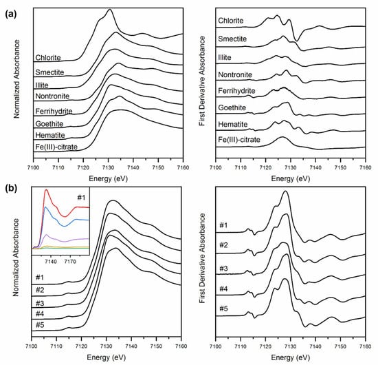
Figure 1.
Normalized XANES (on the left) and corresponding first-derivative spectra (on the right) for standards (a) and sediment samples (b). The inset on the bottom left corner shows an example of LCF (sediment #1): data (in black), best fit (in red), goethite (in blue), smectite (in purple), hematite (orange), ferrihydrite (in green). It is worth to note that the red and black lines perfectly overlap.
LCF was applied to the normalized Fe K-edge XANES spectra (Table 2). Three to four components were used in each fit, as advised by PCA and TT. Moreover, to confirm this pre-analysis, tests using five components were also performed, but since we found no statistical improvement (e.g., better reduced-χ2 or Akaike information criterion), these results were discarded. LCF was also performed on the first derivative XANES spectra. Although previous studies [21,35] underlined the need to perform the LCF on the derivative spectra rather than on the normalized ones, our results did not show significant differences between both approaches. Moreover, the results obtained using LCF of the XANES corroborate those found using EXAFS. The sum of the fitted components was recalculated to 100% after fitting (but not constrained during fitting).
Table 2.
Results for the LCF performed on the normalized Fe K-edge XANES spectra.
All sediment layers were mainly characterized by the presence of smectite (5–23%), goethite (32–92%) and, except for layer #4, hematite (5–40%) (Table 2). Traces of ferrihydrite (2–8%) were found in the first two layers, while illite (14%), Fe-OM (3%) and nontronite (6%) occurred in layers #3, #4 and #5, respectively (Table 2). The fitting revealed goethite and hematite contents in layer #2 and #4, mirroring the mineralogical composition obtained using XRD [12]. The presence of hematite increased with depth, possibly suggesting the formation of more crystalline Fe forms originated from goethite transformation.
The analysis of the Fe K-edge XANES spectrum of these sediment samples by LCF provides a precise estimate of the contribution of Fe(II) and Fe(III) species to its total Fe content. In general, Fe K-edge XANES can well estimate the relative contribution of different mineral classes and groups of organic compounds with different oxidation states of Fe atom in complex matrices such as sediments and paleosols but fails to quantify specific Fe oxyhydroxides or distinct Fe-organic compounds. On the opposite, Fe-EXAFS allows to better distinguish at least ferrihydrite, and this is in agreement with Strawn et al. [36].
3.2. XAS Data Analysis: Fe EXAFS
The Fe K-edge EXAFS spectra of both standards and sediment samples, as well as the corresponding Fourier transforms, are reported in Figure 2.
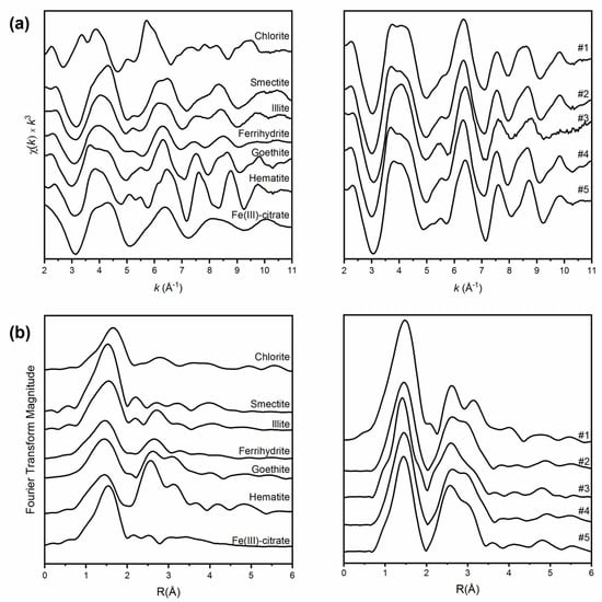
Figure 2.
(a) Normalized Fe EXAFS spectra of both standards (on the left) and sediments (on the right). (b) Corresponding Fourier Transforms of both standards (left) and sediments (right).
Qualitative fits to the EXAFS spectra showed a good match to the goethite reference compound in all sediment samples, and to hematite, especially in layer #5. In fact, the features at 4.0, 5.6 and 8.8 Å−1 in sediments #2 and #4 are similar to those typical of goethite (Figure 2a). Although reported in Figure 2, sediment sample #3 was excluded from the LCF-EXAFS analysis because of the high Mn concentration. In fact, with Mn being the first-lighter atom before Fe and considering the large difference in terms of concentration (42 vs. 6%, respectively; Table 1), the oscillation features relative to Mn EXAFS can be indistinctly observed on the Fe pre-edge, which means the Fe EXAFS element strongly interfered with the Mn signal, making a fair Fe EXAFS analysis impossible.
Fourier transform spectra of sediment samples have similar shapes, with a first and second neighbour peak at 1.55 Å, that seems closer to that of ferrihydrite, and 2.75 Å, similar to that of hematite, respectively, uncorrected for phase shift (Figure 2b).
With the exception of layer #1, Fe (oxyhydr)oxides throughout the whole pedosedimentary record represent >80% of total Fe concentration, with goethite as the most abundant species followed by hematite and ferrihydrite. In detail, quantitative LCF Fe K-edge EXAFS results indicate that these sediments contain significant proportions of goethite in the surface layers (ca. 45–70% of total Fe) compared to the deeper one (<20% in layer #5) (Table 3). Hematite concentration increases with depth, ranging from <10% in layer #1 to >45% in #5, thus confirming the qualitative results and suggesting an increased occurrence of more crystalline Fe forms with depth. The abundance of goethite and hematite in sediments #2 and #4 is also supported by XRD data reported in Puglisi et al. [12]. In addition, high contents in Fe(III)-OM (ca. 20%) occur throughout the whole profile (Table 3), despite the very low organic carbon concentrations characterizing the whole sediment record (Table 1).
Table 3.
Results for LCF performed on the k3-weighted Fe K-edge EXAFS data. Results are expressed in percentage of the fitting components corresponding to experimental spectra of model compounds.
Thus, the identification of Fe species using both EXAFS and XANES suggests the occurrence of diagenetic processes. Samples #2 and #4, in which Fe averages around 46 and 57%, respectively, contain the highest content in goethite that, being a Fe(III) crystalline oxide, would be thus better preserved against Fe oxidizers bacteria compared to amorphous Fe oxides such as ferrihydrite.
3.3. Micro-Raman Spectra of Sediment Samples
Typical micro-Raman spectra of sediment samples, carried out in single-point sampling mode, are reported in Figure 3.
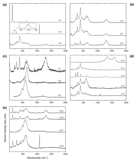
Figure 3.
Raman spectra of sediment samples: (a) sediment #1, with the inset reporting an example of the anatase filtering of the Eg peak in the calcite spectrum (the shoulder at ca. 143 cm−1 highlighted with * is due to the contribution of the Eg mode of anatase); (b) sediment #2; (c) sediment #3; (d) sediment #4; and (e) sediment #5. All the spectra were collected using the DXR2 as discussed in the text, whilst the spectrum S.9 (panel c) was acquired by means of LabRam HR-800 at 0.01 mW to test and avoid any mismatch with the spectra collected with DXR2.
An extensive investigation of sediment sample #1 powder demonstrated that it mainly consists of anatase (TiO2), calcite and goethite (Figure 3a). This finding is in agreement with the XRD results reported in Puglisi et al. [12]. Raman spectra of the different single-phase minerals were acquired thanks to the powder-grain size and to the extremely high spatial resolution of the Raman micro-probe. In particular, the spectrum S.1 is definitely that of anatase, since it shows its typical fingerprint with a very narrow and strong peak at 143 cm−1 and some weaker peaks and bands at 196, 394.5, 514 and 636.5 cm−1 ([37] and ref. therein). The spectrum S.2 displays the typical fingerprint of calcite with a very sharp and strong peak at 1085 cm−1 (A1g) and further peaks at 153.5, 280, 711 and 1435 cm−1 which are classified as Eg modes. Additionally, the weak peak at about 1747.3 cm−1 represents the combination of Eg and A1g modes [38]. In the inset of spectrum S.2, an unexpected shoulder at ca. 143 cm−1 (highlighted with *) is also present, which is the Eg peak of anatase, in form of a small amount embedded into calcite or perhaps mixed to it. Conversely, in the sediment sample #1 it was not possible to get the Raman spectrum of pure goethite, but only composite spectra dominated by the goethite one (see spectrum S.3). In fact, they show peculiar peaks of goethite at 88, 245, 299, 400, 551 and 1003 cm−1 corresponding to the Ag modes, whilst the peak at about 678 cm−1 corresponds to the B2g mode, whose weakness is probably caused by the polarization effect or a different grain orientation [39]. The presence of the spilling Eg mode of anatase at about 143 cm−1 was also observed. Moreover, a recurrent band at about 1310 cm−1 has been noted, which could originate from microscopic regions of coexisting phases (goethite and hematite) inferred from the occurrence of the 2LO mode of hematite [16].
Sediment #2 powder is predominantly composed of the goethite phase, which is detected and reported in Figure 3b (spectra S.4 and S.5). As a matter of fact, the presence of the Ag modes of goethite peaked at 93, 481, 556 cm−1 [39] and the overlap of the Eg modes of hematite (294 and 405 cm−1) probably due to the strong Ag modes of goethite at about 300 and 405 cm−1 were observed. A broad peak of the goethite B2g mode at about 680 cm−1, as a shoulder beside the 1LO mode of the hematite peak at 655 cm−1, was also detected. However, some traces of hematite, whose spectrum is reported in Figure 3b (spectrum S.6), show typical peaks at 245, 293, 405 and 604 cm−1 classified as Eg modes, whilst those at 220 and 499 cm−1 represent the A1g modes, and those at 655 and 1308 cm−1 are usually ascribed to the 1LO and 2LO modes, respectively [40]. These data are in agreement with both EXAFS data (Table 3) and Puglisi et al. [12], who reported goethite (75%) and hematite (25%) as the main mineral components of this sediment layer.
The micro-Raman spectra recorded from sediment sample #3 are displayed in Figure 3c. Typical spectra of hematite were detected in several probed micro-regions of this sample (see spectrum S.7). However, being the most enriched in Mn (42%) [12,24], sediment #3 coherently shows single-phase spectra of todorokite, characterized by a single band centered at about 650 cm−1 with two weak shoulders at 576 and 501 cm−1 (see spectrum S.8). Even though our positions differ from about 10 to 20 cm−1 compared to other case studies [41,42,43,44], we observe a spectral profile quite similar to that reported in Bernardini et al. [45]. Although the peak position does not provide a self-consistent method on the todorokite phase discrimination (as discussed in [45]), we found confirmation in our XRD analysis [12,24]. Additionally, spectra showing a dominant peak at about 592 cm−1 with a shoulder at 610 cm−1 and wide bands at 1097 and 1210 cm−1, together a secondary peak at about 495 cm−1, probably represent a Mn oxide or hydroxide phase (spectrum S.9). The presence of these wide frames suggests a structure strongly affected by long-range disorder or micro-clustering, originating wide peaks and bands [45]. However, the phase-identification amongst the Mn oxides structures represents a non-trivial procedure since the Raman modes are strongly influenced firstly by the polarization effect (which is a poorly investigated field for this materials) and secondly by the oxidation state of Mn determining its distribution inside the structure [46]. In addition, the excitation wavelength and the laser power used for the experiments play a crucial role in the Raman response in characterizing Mn oxides (see [44] and ref. therein). Strong affinities were also found with asbolane of an Al-poor term investigated by Burlet and Vanbrabant [47] (sample RB3352), slightly different to those discussed in Post et al. [48], who observed spectra dominated by the so-called D peak centred near 597 cm−1 as well as other low- and high-shifted peaks (sample 103709), and a match with samples used in parametrizing and validating the Mn oxide identification-approach proposed by Mulè et al. [49].
In sediment sample #4 (Figure 3d), graphitic-like C (spectrum S.10) were identifiable by the typical D and G bands located at 1334 and 1591 cm−1, respectively [50]. Additionally, spectra of the single-phase are rarely detected, such as in the spectrum of the S.12 of the hematite, easily identified due the characteristic peaks described above. In this sediment, the goethite spectra often show components of different secondary phases such as calcite (spectrum S.14), characterized by its sharp peak at about 1085 cm−1. Finally, the co-presence of the band centered at 592 cm−1 probably belongs to the same Mn oxide detected in sediment #3 (spectrum S.13). Therefore, Raman spectrum of sediment #4 provides a more complex picture compared to that obtained using XRD (almost exclusively goethite) [12] and XANES.
Raman spectra of sediment sample #5 (Figure 3e) were very similar to sample #1 but still presented some characteristic spectral features of both layer #3 and #4. Indeed, spectra S.15 and S.16 (Figure 3e) revealed the presence of anatase (fingerprint at 143 cm−1), hematite (through its 2LO mode peaked at 1308 cm−1) and todorokite (single band centered at about 650 cm−1, as for sediment #3). Additionally, the same Mn oxide (see spectrum S.17) having a peak at about 592 cm−1 with a secondary one at about 495 cm−1 was found. Another similarity with sediment #1 can be observed in spectrum S.18 whereby both anatase and calcite were recorded and identified through their typical fingerprints (i.e., the peak at 143 cm−1 for anatase and that at 1085 cm−1, for calcite, respectively). Additionally, for this layer, Raman data were in good agreement with those obtained by XRD [12].
3.4. Which Techniques Are Better Suited to Reveal Ferrihydrite Occurrence?
Both XRD [12] and Raman spectroscopy (this study) were not able to reveal the presence of ferrihydrite. In detail, Raman spectra of synthetic ferrihydrite consist of both broad and rather weak bands at ~361, ~508, ~707, and ~1045 cm−1 [51]. The strongest band at ~707 and weaker bands at ~361 and ~508 cm−1 have been also confirmed by previous studies [17,52]. However, no studies have reported another strong band at ~1045 cm−1, which Das and Hendry [51] clearly identified even after five repeated scans at a low laser power (0.1%). Jia et al. [53] reported well-resolved ferrihydrite bands at 222, 289, and 407 cm−1 and a weak band at 606 cm−1, but none of these are consistent with our results. As reported by Mazzetti and Thistlethwaite [52], the poor crystallinity of both 2- and 6-line ferrihydrite leads to a general band broadening, followed by an intensity weakening. This condition could be prone to unresolved band over-imposition or strong filtering from neighboring mineral phases. Moreover, the same authors [52] reported bands at ~220, ~286, and ~405 cm−1 resulting from the thermal transformation of ferrihydrite to hematite due to increased laser power (from 0.1 to 100%). Indeed, the transformation of ferrihydrite in hematite can be direct (in the case of the 6-line type) or involve the progressive replacement of the original 710 cm−1 band first with the maghemite bands at ~700 and ~ 650 cm−1, and second with the strong 612 cm−1 band of hematite (in the case of the 2-line type). This highlights the very high thermal instability of this Fe mineral phase. A further indication of the lack of ferrihydrite identification by RS may also be ascribed to the fluorescence effect from its interaction with the organic matter during the scattering process as shown in Hanesch et al. [17].
Therefore, Fe (oxyhydr)oxides, and ferrihydrite in particular, can be extremely difficult to identify or distinguish unless multiple analytical techniques are used. Most of the literature reports fail to parameterize the sample morphology, making it difficult to understand how morphology affects spectral characteristics across techniques. Here, Fe EXAFS and XANES and RS results were presented and the feature positions of Fe species occurring in the sediments under investigation were compared to Fe phases from the literature, including previous XRD data [12]. Overall, XAS and RS may provide better species identification and detection limits than XRD. Raman spectroscopy is suitable in identifying and distinguishing goethite, and hematite; unfortunately, laser irradiation exploited in RS can lead to the transformations of Fe phases, so that low-laser powers must be used to avoid phase changes. On the other hand, nanophase magnetite, maghemite, and ferrihydrite have similar Raman spectra, showing an important broadening and overlapping of the bands which often results in remarkable shifts of the band centroid [54].
As previously reported, LCF on the derivative XANES spectra was also carried out, because goethite and ferrihydrite could not be distinguished with LCF conducted on either the whole Fe K-edge XANES spectrum or its pre-edge feature, whereas LCF on Fe-EXAFS spectra is best suited to distinguish ferrihydrite, goethite and hematite. Therefore, while the challenges of phase identification in Fe (oxyhydr)oxides are many, the application of some or all of these techniques together can provide sufficient evidence for the identification and discrimination of Fe phases.
3.5. Further ‘Tips’ from Thermal Analysis
The simultaneous TGA-DSC analysis clearly underlines similarities between sediment samples #1 and #5, as well as between #2 and #4 (Figure 4a).
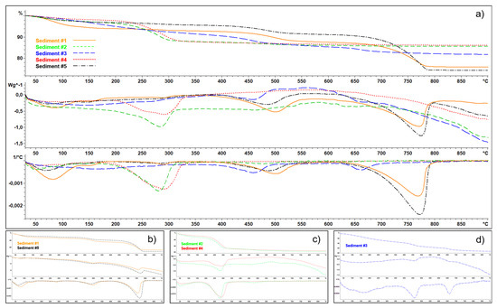
Figure 4.
Thermogravimetric (TG; in the top), differential scanning calorimetry (DSC; in the middle) and first derivative (in the bottom) curves of: (a) all sediments; (b) sediment #1 vs. #5; (c) sediment #2 vs. #4; and (d) sediment #3.
According to elemental analysis (CHNS) and XRD data reported in Puglisi et al. [12], sediments #1 and 5 show an inorganic carbon content of 3 and 4%, respectively (Table 1), occurring mainly as calcite (70–80%), as also confirmed in the present study using RS. This is in agreement with both TGA curves, showing a weight loss (WL) of 16–20% between 550–800 °C, and DSC ones, characterized by an evident endothermic peak between 750 and 800 °C, with a maximum around 765 °C (Figure 4b). These trends typically describe the thermal decomposition of calcite. In addition, a minor endothermic shoulder occurs in DSC around 500 °C.
Sediments #2 and 4 (Figure 4c) show a major WL (10%) between 200 and 350 °C, probably due to the decomposition of goethite and ferrihydrite, occurring at high contents in these samples (see Table 3 and [12]), into hematite. According to Da Costa et al. [55], this WL has been termed as structural hydroxyl, bulk dehydroxylation, intrinsic dehydroxylation, dehydroxylation, non-stoichiometric hydroxyl units, strongly bounded water and OH groups. The WL in the region <200 °C is due to bulk dehydration and surface dehydration/dehydroxylation, nonstoichiometric water from bulk and surface, weakly bound OH groups, surface-bound and bulk-sequestered water, loosely bound hydroxyl units, dehydration from hydrogen bonded water or the dehydroxylation of the surface [55]. Both the first derivative curve and the DSC underline such an endothermic reaction.
Sediment #3 is mainly constituted by Mn oxides (todorokite with possible traces of asbolan), as also confirmed by RS, and Fe oxides (24%), mainly as goethite and hematite (Table 2 and [12]). The TGA results for todorokite showed that the mass decreased almost steadily from the starting temperature to ~700 °C (Figure 4d). The WL observed between 50–105 °C (1.5%) can be attributed to the loss of water physically absorbed on the surface and that between 105–250 °C (5%) to the one bound in the tunnels [56]. Finally, the WL at 250–700 °C (12%) can be attributed to the decomposition of todorokite and oxygen evolution upon heating. The first derivative of the TGA curve underlines two sudden weight losses, peaking at 460 and 660 °C, possibly indicating the collapse of the tunnel structure owing to significant structural phase transition [56,57].
4. Conclusions
The pedosediment record under investigation represents a peculiar stratigraphic series showing complex features mainly related to the Fe dynamic and caused by redox cycles. Therefore, it offered a unique opportunity to study Fe mineral composition using both Fe-XANES and Fe-EXAFS as well as RS.
Generally speaking, the challenges of phase identification in Fe (oxyhydr)oxides are many, but the application of multiple techniques provided sufficient and complementary evidence for the identification and discrimination of Fe phases. In detail, Raman (this study) and XRD (previous study) spectroscopies seem to be not well suited for the identification of some Fe-bearing minerals (such as ferrihydrite or clay minerals) besides Fe-OM. In contrast, Fe K-edge XANES can fairly well estimate the relative contribution of different mineral classes and Fe-OM compounds with different oxidation states of the Fe atom. The combination of Fe-XANES and EXAFS allowed for a complete speciation of Fe. In detail, goethite is the most abundant, followed by hematite and ferrihydrite, thus confirming that redox cycling of Fe occurred in these sediments. Quantitative LCF Fe K-edge EXAFS results indicate that these sediments contain significant proportions of goethite in the surface layers (up to 70%) compared to the deeper one (<20%). The hematite concentration increases with depth, ranging from <10% in the top layer to >45% in the bottom one, thus suggesting an increase in more crystalline Fe forms with depth, which would be better preserved against Fe oxidizers bacteria compared to amorphous Fe oxides such as ferrihydrite. For both goethite and hematite, XAS data were in sufficient agreement with XRD and RS, especially for layers #2 and #4. In addition, despite the extremely low organic carbon content throughout the sediment record, organically complexed Fe(III) represented around 20% of the total Fe in all layers, thus underlining the important rule of microbial communities even in such an extreme environment. Finally, thermal analysis can also be a useful tool to unravel some mineralogical components in sediment samples.
Author Contributions
Conceptualization, B.G., M.C., G.M. and C.Z.; methodology, B.G., M.C., D.O.d.S. and G.M.; formal analysis, B.G., M.C., D.O.d.S., G.M. and C.Z.; data curation, B.G., M.C., D.O.d.S., G.M., G.A. and C.Z.; writing—original draft preparation, B.G., M.C., G.M. and C.Z.; writing—review and editing, B.G., M.C., D.O.d.S., G.M., G.A. and C.Z.; supervision, G.M., G.A. and C.Z. All authors have read and agreed to the published version of the manuscript.
Funding
This research received no external funding.
Acknowledgments
The authors would like to thank Marco Giarola, Technological Platform Center (CPT) of the University of Verona, for the skilful help in setting the experimental apparatuses used for micro-Raman measurements.
Conflicts of Interest
The authors declare no conflict of interest.
References
- Yaalon, D.H. Soils in the Mediterranean region: What makes them different? Catena 1997, 28, 157–169. [Google Scholar] [CrossRef]
- Colombo, C.; Torrent, J. Relationships between aggregation and iron oxides in Terra Rossa soils from Southern Italy. Catena 1991, 18, 51–59. [Google Scholar] [CrossRef]
- Atalay, I. Red Mediterranean soils in some karstic regions of Taurus mountains, Turkey. Catena 1997, 28, 247–260. [Google Scholar] [CrossRef]
- Cabadas-Báez, H.; Solleiro-Rebolledo, E.; Sedov, S.; Pi-Puig, T.; Gama-Castro, J. Pedosediments of karstic sinkholes in the eolianites of NE Yucatán: A record of Late Quaternary soil development, geomorphic processes and landscape stability. Geomorphology 2010, 122, 323–337. [Google Scholar] [CrossRef]
- Priori, S.; Costantini, E.A.C.; Capezzuoli, E.; Protano, G.; Hilgers, A.; Sauer, D.; Sandrelli, F. Pedostratigraphy of Terra Rossa and Quaternary geological evolution of a lacustrine limestone plateau in central Italy. J. Plant Nutr. Soil Sci. 2008, 171, 509–523. [Google Scholar] [CrossRef]
- Canfield, D.E. The early history of atmospheric oxygen: Homage to Robert M. Garrels. Annu. Rev. Earth Planet. Sci. 2005, 33, 1–36. [Google Scholar] [CrossRef] [Green Version]
- Lyons, T.W.; Severmann, S. A critical look at iron paleoredox proxies: New insights from modern euxinic marine basins. Geochim. Cosmochim. Acta 2006, 70, 5698–5722. [Google Scholar] [CrossRef]
- Eze, P.; Meadows, M. Mineralogy and micromorphology of a late Neogene paleosol sequence at Langebaanweg, South Africa: Inference of paleoclimates. Palaeogeogr. Palaeoclimatol. Palaeoecol. 2014, 409, 205–216. [Google Scholar] [CrossRef]
- Sheldon, N.D.; Tabor, N.J. Quantitative paleoenvironmental and paleoclimatic reconstruction using paleosols. Earth-Sci. Rev. 2009, 95, 1–52. [Google Scholar] [CrossRef]
- Zaccone, C.; Quideau, S.; Sauer, D. Soils and paleosols as archives of natural and anthropogenic environmental changes. Eur. J. Soil Sci. 2014, 65, 403–405. [Google Scholar] [CrossRef]
- Nukazawa, K.; Itakiyo, T.; Ito, K.; Sato, S.; Oishi, H.; Suzuki, Y. Mineralogical fingerprint to characterize spatial distribution of coastal and riverine sediments in southern Japan. Catena 2021, 203, 105823. [Google Scholar] [CrossRef]
- Puglisi, E.; Squartini, A.; Terribile, F.; Zaccone, C. Pedosedimentary and microbial investigation of a karst sequence record. Sci. Total Environ. 2022, 810, 151297. [Google Scholar] [CrossRef] [PubMed]
- Schwertmann, U.; Taylor, R.M. Iron oxides. In Minerals in Soil Environments, 2nd ed.; Dixon, J.B., Weed, S.B., Eds.; SSSA Book Series; Wiley: Hoboken, NJ, USA, 1989; pp. 379–438. [Google Scholar]
- Slotznick, S.P.; Sperling, E.A.; Tosca, N.J.; Miller, A.J.; Clayton, K.E.; van Helmond, N.A.G.M.; Slomp, C.P.; Swanson-Hysell, N.L. Unraveling the mineralogical complexity of sediment iron speciation using sequential extractions. Geochem. Geophys. Geosyst. 2020, 21, e2019GC008666. [Google Scholar] [CrossRef]
- de Faria, D.L.A.; Venâncio Silva, S.; De Oliveira, M.T. Raman microspectroscopy of some iron oxides and oxyhydroxides. J. Raman Spectrosc. 1997, 28, 873–878. [Google Scholar] [CrossRef]
- de Faria, D.L.A.; Lopes, F.N. Heated goethite and natural hematite: Can Raman spectroscopy be used to differentiate them? Vib. Spectrosc. 2007, 45, 117–121. [Google Scholar] [CrossRef]
- Hanesch, M. Raman spectroscopy of iron oxides and (oxy)hydroxides at low laser power and possible applications in environmental magnetic studies. Geophys. J. Int. 2009, 177, 941–948. [Google Scholar] [CrossRef]
- Bastians, S.; Crump, G.; Griffith, W.P.; Withnall, R. Raspite and studtite: Raman spectra of two unique minerals. J. Raman Spectrosc. 2004, 35, 726–731. [Google Scholar] [CrossRef]
- Martens, W.; Frost, R.L.; Williams, P.A. Molecular structure of the adelite group of minerals—A Raman spectroscopic study. J. Raman Spectrosc. 2003, 34, 104–111. [Google Scholar] [CrossRef] [Green Version]
- Giannetta, B.; Oliveira de Souza, D.; Aquilanti, G.; Celi, L.; Said-Pullicino, D. Redox-driven changes in organic C stabilization and Fe mineral transformations in temperate hydromorphic soils. Geoderma 2022, 406, 115532. [Google Scholar] [CrossRef]
- O’Day, P.A.; Rivera, N.; Root, R.; Carroll, S.A. X-ray absorption spectroscopic study of Fe reference compounds for the analysis of natural sediments. Am. Miner. 2004, 89, 572–585. [Google Scholar] [CrossRef]
- Root, R.A.; Vlassopoulos, D.; Rivera, N.A.; Rafferty, M.T.; Andrews, C.; O’Day, P.A. Speciation and natural attenuation of arsenic and iron in a tidally influenced shallow aquifer. Geochim. Cosmochim. Acta 2009, 73, 5528–5553. [Google Scholar] [CrossRef]
- Noel, V.; Marchand, C.; Juillot, F.; Ona-Nguema, G.; Viollier, E.; Marakovic, G.; Olivi, L.; Delbes, L.; Gelebart, F.; Moring, G. EXAFS analysis of iron cycling in mangrove sediments downstream a lateritized ultramafic watershed (Vavouto Bay, New Caledonia). Geochim. Cosmochim. Acta 2014, 136, 211–228. [Google Scholar] [CrossRef]
- Bletsa, E.; Zaccone, C.; Miano, T.; Terzano, R.; Deligiannakis, Y. Natural Mn-todorokite as an efficient and green azo dye-degradation catalyst. Environ. Sci. Poll. Res. 2020, 27, 9835–9842. [Google Scholar] [CrossRef]
- Doglioni, C.; Mongelli, F.; Pieri, P. The Puglia uplift (SE Italy): An anomaly in the foreland of the Apenninic subduction due to buckling of a thick continental lithosphere. Tectonics 1994, 13, 1309–1321. [Google Scholar] [CrossRef]
- De Santis, V.; Caldara, M.; de Torres, T.; Ortiz, J.E. Stratigraphic units of the Apulian Tavoliere plain (Southern Italy): Chronology, correlation with marine isotope stages and implications regarding vertical movements. Sediment. Geol. 2010, 228, 255–270. [Google Scholar] [CrossRef] [Green Version]
- Aquilanti, G.; Giorgetti, M.; Dominko, R.; Stievano, L.; Arčon, I.; Novello, N.; Olivi, L. Operando characterization of batteries using X-ray absorption spectroscopy: Advances at the beamline XAFS at synchrotron Elettra. J. Phys. D Appl. Phys. 2017, 50, 074001. [Google Scholar] [CrossRef]
- Di Cicco, A.; Aquilanti, G.; Minicucci, M.; Principi, E.; Novello, N.; Cognigni, A.; Olivi, L. Novel XAFS capabilities at ELETTRA synchrotron light source. J. Phys. Conf. Ser. 2009, 190, 012043. [Google Scholar] [CrossRef]
- Giannetta, B.; Plaza, C.; Siebecker, M.G.; Aquilanti, G.; Vischetti, C.; Plaisier, J.R.; Juanco, M.; Sparks, D.L.; Zaccone, C. Iron speciation in organic matter fractions isolated from soils amended with biochar and organic fertilizers. Environ. Sci. Technol. 2020, 54, 5093–5101. [Google Scholar] [CrossRef]
- Giannetta, B.; Siebecker, M.G.; Zaccone, C.; Plaza, C.; Rovira, P.; Vischetti, C.; Sparks, D.L. Iron(III) fate after complexation with soil organic matter in fine silt and clay fractions: An EXAFS spectroscopic approach. Soil Tillage Res. 2020, 200, 104617. [Google Scholar] [CrossRef]
- Westre, T.E.; Kennepohl, P.; DeWitt, J.G.; Hedman, B.; Hodgson, K.O.; Solomon, E.I. A multiplet analysis of Fe K-edge 1s → 3d pre-edge features of iron complexes. J. Am. Chem. Soc. 1997, 119, 6297–6314. [Google Scholar] [CrossRef]
- Wilke, M.; Farges, F.; Petit, P.E.; Brown, G.E.; Martin, F. Oxidation state and coordination of Fe in minerals: An Fe K-XANES spectroscopic study. Am. Miner. 2001, 86, 714–730. [Google Scholar] [CrossRef]
- Farges, F.; Rossano, S.; Lefrère, Y.; Wilke, M.; Brown, G.E. Iron in silicate glasses: A systematic analysis of pre-edge, XANES and EXAFS features. Phys. Scr. 2005, T115, 957–959. [Google Scholar] [CrossRef]
- Galoisy, L.; Calas, G.; Arrio, M.A. High-resolution XANES spectra of iron in minerals and glasses: Structural information from the pre-edge region. Chem. Geol. 2001, 174, 307–319. [Google Scholar] [CrossRef]
- Prietzel, J.; Thieme, J.; Eusterhues, K.; Eichert, D. Iron speciation in soils and soil aggregates by synchrotron-based X-ray microspectroscopy (XANES, μ-XANES). Eur. J. Soil Sci. 2007, 58, 1027–1041. [Google Scholar] [CrossRef]
- Strawn, D.; Doner, H.; Zavarin, M.; McHugo, S. Microscale investigation into the geochemistry of arsenic, selenium, and iron in soil developed in pyritic shale materials. Geoderma 2002, 108, 237–257. [Google Scholar] [CrossRef]
- Giarola, M.; Sanson, A.; Monti, F.; Mariotto, G.; Bettinelli, M.; Speghini, A.; Salviulo, G. Vibrational dynamics of anatase TiO2: Polarized Raman spectroscopy and ab initio calculations. Phys. Rev. B-Condens. Matter Mater. Phys. 2010, 81, 174305. [Google Scholar] [CrossRef]
- Rutt, H.N.; Nicola, J.H. Raman spectra of carbonates of calcite structure. J. Phys. C Solid State Phys. 1974, 7, 4522–4528. [Google Scholar] [CrossRef]
- Abrashev, M.V.; Ivanov, G.V.; Stefanov, B.S.; Todorov, N.D.; Rosell, J.; Skumryev, V. Raman spectroscopy of alpha-FeOOH (goethite) near antiferromagnetic to paramagnetic phase transition. J. Appl. Phys. 2020, 127, 205108. [Google Scholar] [CrossRef]
- Marshall, C.P.; Dufresne, W.J.B.; Rufledt, C.J. Polarized Raman spectra of hematite and assignment of external modes. J. Raman Spectrosc. 2020, 51, 1522–1529. [Google Scholar] [CrossRef]
- Feng, X.H.; Tan, W.F.; Liu, F.; Wang, J.B.; Ruan, H.D. Synthesis of todorokite at atmospheric pressure. Chem. Mater. 2004, 16, 4330–4336. [Google Scholar] [CrossRef]
- Julien, C.; Massot, M.; Baddour-Hadjean, R.; Franger, S.; Bach, S.; Pereira-Ramos, J.P. Raman spectra of birnessite manganese dioxides. Solid State Ionics 2003, 159, 345–356. [Google Scholar] [CrossRef]
- Julien, C.M.; Massot, M.; Poinsignon, C. Lattice vibrations of manganese oxides: Part I. Periodic structures. Spectrochim. Acta-Part A Mol. Biomol. Spectrosc. 2004, 60, 689–700. [Google Scholar] [CrossRef]
- Post, J.E.; McKeown, D.A.; Heaney, P.J. Raman spectroscopy study of manganese oxides: Tunnel structures. Am. Miner. 2020, 105, 1175–1190. [Google Scholar] [CrossRef]
- Bernardini, S.; Bellatreccia, F.; Casanova Municchia, A.; Della Ventura, G.; Sodo, A. Raman spectra of natural manganese oxides. J. Raman Spectrosc. 2019, 50, 873–888. [Google Scholar] [CrossRef]
- Bernardini, S.; Bellatreccia, F.; Della Ventura, G.; Sodo, A. A reliable method for determining the oxidation state of manganese at the microscale in Mn oxides via Raman Spectroscopy. Geostand. Geoanal. Res. 2021, 45, 223–244. [Google Scholar] [CrossRef]
- Burlet, C.; Vanbrabant, Y. Study of the spectro-chemical signatures of cobalt-manganese layered oxides (asbolane-lithiophorite and their intermediates) by Raman spectroscopy. J. Raman Spectrosc. 2015, 46, 941–952. [Google Scholar] [CrossRef]
- Post, J.E.; McKeown, D.A.; Heaney, P.J. Raman spectroscopy study of manganese oxides: Layer structures. Am. Miner. 2021, 106, 351–366. [Google Scholar] [CrossRef]
- Mulè, G.; Burlet, C.; Vanbrabant, Y. Automated curve fitting and unsupervised clustering of manganese oxide Raman responses. J. Raman Spectrosc. 2017, 48, 1665–1675. [Google Scholar] [CrossRef]
- Dillon, R.O.; Woollam, J.A.; Katkanant, V. Use of Raman scattering to investigate disorder and crystallite formation in as-deposited and annealed carbon films. Phys. Rev. B 1984, 29, 3482–3489. [Google Scholar] [CrossRef]
- Das, S.; Hendry, M.J. Application of Raman spectroscopy to identify iron minerals commonly found in mine wastes. Chem. Geol. 2011, 290, 101–108. [Google Scholar] [CrossRef]
- Mazzetti, L.; Thistlethwaite, P.J. Raman spectra and thermal transformations of ferrihydrite and schwertmannite. J. Raman Spectrosc. 2002, 33, 104–111. [Google Scholar] [CrossRef]
- Jia, Y.; Xu, L.; Fang, Z.; Demopoulos, G.P. Observation of surface precipitation of arsenate on ferrihydrite. Environ. Sci. Technol. 2006, 40, 3248–3253. [Google Scholar] [CrossRef] [PubMed]
- Sklute, E.C.; Kashyap, S.; Dyar, M.D.; Holden, J.F.; Tague, T.; Wang, P.; Jaret, S.J. Spectral and morphological characteristics of synthetic nanophase iron (oxyhydr)oxides. Phys. Chem. Miner. 2018, 45, 1–26. [Google Scholar] [CrossRef] [PubMed]
- Da Costa, G.M.; Novack, K.M.; Elias, M.M.C.; Da Cunha, C.C.R.F. Quantification of moisture contents in iron and manganese ores. ISIJ Int. 2013, 53, 1732–1738. [Google Scholar] [CrossRef] [Green Version]
- Bish, D.L.; Post, J.E. Thermal behavior of complex, tunnel-structure manganese oxides. Am. Miner. 1989, 74, 177–186. [Google Scholar]
- Shen, Y.F.; Zerger, R.P.; Deguzman, R.N.; Suib, S.L.; McCurby, L.; Potter, D.I.; O’Young, C.L. Manganese oxide octahedral molecular sieves: Preparation, characterization, and applications. Science 1993, 260, 511–515. [Google Scholar] [CrossRef]
Publisher’s Note: MDPI stays neutral with regard to jurisdictional claims in published maps and institutional affiliations. |
© 2022 by the authors. Licensee MDPI, Basel, Switzerland. This article is an open access article distributed under the terms and conditions of the Creative Commons Attribution (CC BY) license (https://creativecommons.org/licenses/by/4.0/).