Article

Path Analysis of Sea-Level Rise and Its Impact

Department of Applied Mathematics and Statistics, State University of New York at Stony Brook, Stony Brook, NY 11794, USA
*
Author to whom correspondence should be addressed.
These authors contributed equally to this work.
Stats 2022, 5(1), 12-25; https://doi.org/10.3390/stats5010002
Submission received: 22 October 2021 / Revised: 13 December 2021 / Accepted: 17 December 2021 / Published: 24 December 2021

Abstract

:
Global sea-level rise has been drawing increasingly greater attention in recent years, as it directly impacts the livelihood and sustainable development of humankind. Our research focuses on identifying causal factors and pathways on sea level changes (both global and regional) and subsequently predicting the magnitude of such changes. To this end, we have designed a novel analysis pipeline including three sequential steps: (1) a dynamic structural equation model (dSEM) to identify pathways between the global mean sea level (GMSL) and various predictors, (2) a vector autoregression model (VAR) to quantify the GMSL changes due to the significant relations identified in the first step, and (3) a generalized additive model (GAM) to model the relationship between regional sea level and GMSL. Historical records of GMSL and other variables from 1992 to 2020 were used to calibrate the analysis pipeline. Our results indicate that greenhouse gases, water, and air temperatures, change in Antarctic and Greenland Ice Sheet mass, sea ice, and historical sea level all play a significant role in future sea-level rise. The resulting 95% upper bound of the sea-level projections was combined with a threshold for extreme flooding to map out the extent of sea-level rise in coastal communities using a digital coastal tracker.

1. Introduction

Since the industrial age, global mean sea-level (GMSL) rise has become a persistent trend that has greatly accelerated within the last two and a half decades [1]. This is largely due to thermal expansion, or increased temperature leading to a greater volume of water per unit mass, and the melting of glaciers and land-based ice caps [2]. The IPCC reports that beyond 2050, anthropogenic activities such as increased greenhouse emissions could result in further climate warming and a substantial increase in GMSL [3]. Additionally, high tide floods are becoming more frequent and reaching farther inland [4]. Many large cities located along coastal regions are likely to suffer drastic socioeconomic impacts from sea-level rise and high tide flooding. Hundreds of coastal communities, home to over 634 million people [5], are likely to face increased flooding that would devastate homes, lives, and communities, as seen in recent major flooding occurrences in Miami, New York City, and New Orleans (Figure 1).
The inherent relationship between GMSL and predictors such as glaciers, ocean circulation, and thermal expansion is not fully understood. Several recent studies were proposed in an attempt to simplify the relationship [6,7]. These approaches are able to recognize a trend or inherent relationship, but an estimate of the underlying causal pathways for long-term projection of GMSL is not given. Some researchers made predictions within the next 100 years [8,9,10]. Based on these studies, the GMSL rise by 2100 is estimated to be in the range between 60 to 130 cm. However, such models are either overly simplified, lacking the incorporation of essential causal relations, or overly complicated, featuring sophisticated atmospheric and climate models that can only be shown as a black box. This is a significant gap between existing analyses and public comprehension—and hence public actions.
“Seeing is believing”—if we, as unbiased citizen scientists, could utilize available public data, design a comprehensive analysis pipeline to uncover the underlying causal relations and predict GMSL on our own, we would then be more convinced of the impending danger and thus take up actions to control for the causal links, such as the man-made greenhouse gas emission, to help curb this chain reaction. To this end, we have proposed a three-step statistical analysis pipeline (Figure 2) to model and predict the global mean sea level. Firstly, a dynamic structural equation model (dSEM) is used to establish a pathway model to evaluate the effects of greenhouse gases, increasing air and water temperatures, decreasing Antarctic and Greenland Ice Sheet size, and decreasing sea ice. This pathway can help gauge the underlying pathway towards sea-level rise and help confirm whether the increase in greenhouse gases was responsible for the chain reaction that resulted in increased air temperature, which thus increases water temperature, the melting of ice sheets and ice caps, which then contributes to sea-level rise. In addition, we aim to analyze the relationship between sea ice, which has no direct contribution to sea-level rise, and the various predictors in our model. In our second procedure, we used a vector autoregression model (VAR) with more lags to more accurately forecast global mean sea-level rise based on direct causal factors identified through the SEM analysis. In our third procedure, we used a generalized additive model (GAM) in order to link global mean sea level to regional coastal areas in the United States and forecast regional sea level changes. Lastly, our predictions were used to analyze the extent of extreme coastal flooding by 2050 and 2100 using tidal gauge data in coastal urban areas such as New York City, Miami, and New Orleans.

2. Data and Methods

2.1. Data

All data were recorded in monthly averages and available in publicly accessible repositories. To gather data on sea-level rise, we used NASA’s sea-level data, which were generated through multi-mission ocean altimetry [11]. We gathered the data for the monthly average sea ice extent in the Northern Hemisphere, mainly composed of Arctic sea ice, through the NSIDC (National Snow & Ice Data Center) [12]. The Greenland and Antarctic Ice Sheet mass losses were accessed through the IMBIE (Ice sheet Mass Balance Inter-comparison Exercise) datasets [13] and NASA [14]. The data for the average monthly air and water (sea surface) temperatures were accessed through Berkeley Earth [15]. The atmospheric CO2 data were taken from the Mauna Loa Observatory, as part of the Scripps CO2 program [16]. The CH4 and N2O data were taken from 2degreesinstitute [17]. Lastly, the local tidal gauge stations for coastal areas in New York, Miami, and New Orleans were accessed through the NOAA Center for Operational Oceanographic Products and Services [18].
Prior to analysis, all monthly data were combined to range from 1992 to 2020. The Water Temperature and Air Temperature represent the global average temperature. They are calculated by adding the corresponding global average water/air temperature anomalies and their baselines, which are the monthly means of the global average water/air temperature. Data for the Antarctic and Greenland Ice Sheet mass loss ranged from 1992 to 2002 were taken from NSIDC [13], and those ranging from 2002 to 2020 were from NASA [14] after removing the seasonal effect.

2.2. Step 1: The Dynamic SEM Model

Structural equation modeling (SEM) is a multivariate technique [19] towards the confirmatory analysis of causal associations among a set of variables [20,21]. Even so, SEM is flexible enough to incorporate exploratory analyses of data as unsure pathways can be kept in the hypothesis to be validated by the analysis. SEM assumes that proposed relations among variables can be represented in a set of structural regression equations and that these relations can be represented pictorially in the form of a path diagram [19,22].
The unified (or dynamic) structural equation model [22], also known as VAR-SEM model or MAR–SEM model, can be used to analyze the proposed causal associations among a set of time-series variables by incorporating both the contemporaneous relations as well as the longitudinal relations represented by the VAR model. Specifically, longitudinal temporal relations are defined as relationships between regions involving different time points, while contemporaneous relations reflect relationships between regions at the same time point. Let y j t be the j th measured at time t ,   j = 1 ,   2 ,   ,   m . The m-dimensional multivariate autoregressive process of order p (VAR (p)) with an added component of contemporaneous relations can be written as:
y t = c + A y t + ϕ 1 y t 1 + ϕ 2 y t 2 + + ϕ p y t p + ϵ t ,
Here y t = y 1 t , y 2 t , , y n t ′ is the n × 1 vector of observed variables measured at time t, ϵ t is the n × 1 vector white noise with zero-mean, A is the parameter matrix of the contemporaneous relations, and ϕ i , i   = 1, 2, ..., p is a series of n × n parameter matrices representing the longitudinal relations.
There is no latent variable in our VAR(1)-SEM model. In our model, there are six observed variables in total, which are GMSL, Sum (glacier) Mass, Sea Ice, Water Temperature, Air Temperature, and Greenhouse Gas. The definition of the variables is shown in Table 1.
As it is a VAR(1)-SEM model, each variable has two states in the model, at time t and time t − 1. Thus, there are 6 × 2 = 12 variables in the VAR(1)-SEM totally. If we use the original data Sum Mass to estimate the parameters in the VAR-SEM model, the model will fail to converge, as the value of Sum Mass is 1000 times larger than others. Thus, we take the natural log on the Sum Mass (cumulative glacier mass change) plus 8000 towards the VAR(1)-SEM.
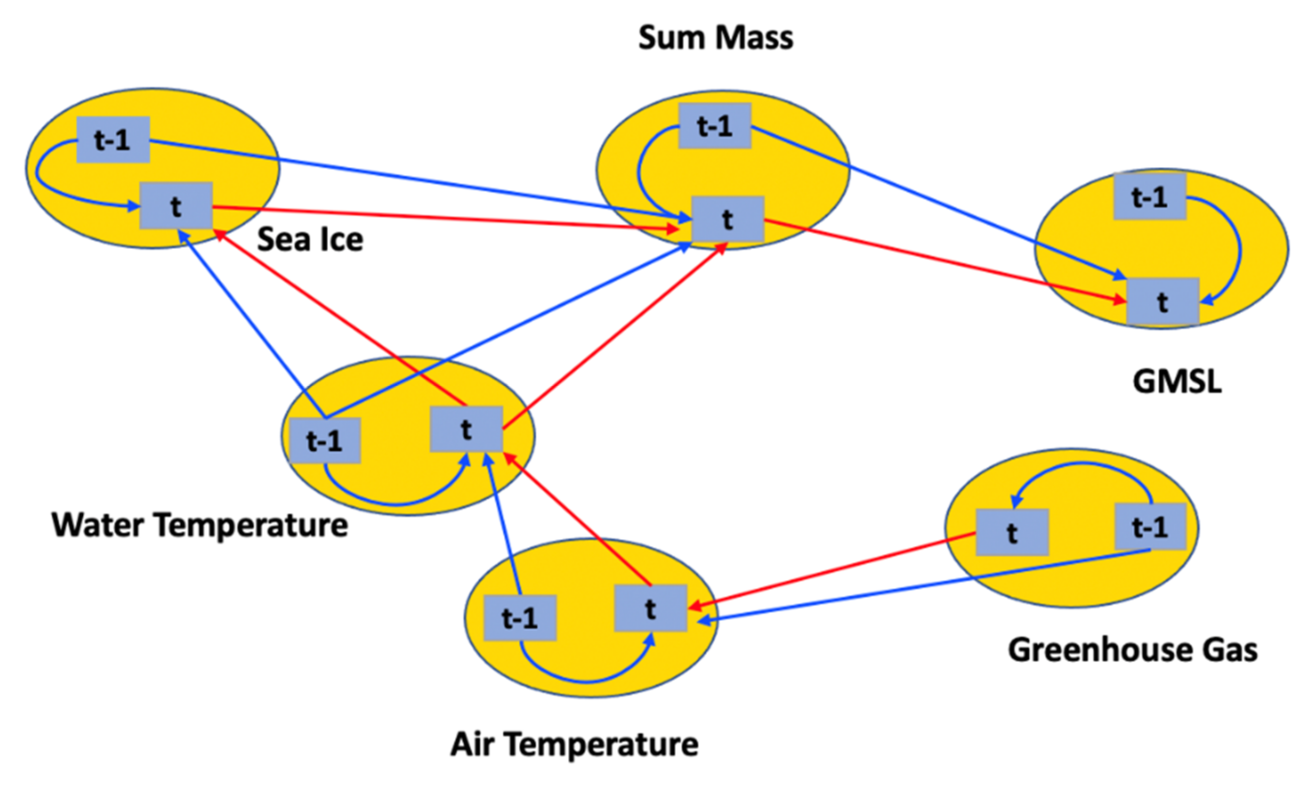
Based on extensive literature review, we proposed a climate model as follows. First, increasing Greenhouse Gas would lead to an increase in Air Temperature. The increase in Air Temperature would correlate to rising Water Temperature. Increase in Air/Water Temperature would then lead to the loss of Sea Ice and Sum Mass (glacier mass). The loss of glacier mass would in turn increase the Global Mean Sea Level.
Based on the above induction and the model parsimony principle, our hypothesis for the dynamic SEM was generated with the longitudinal relations only involving the lag one pathways, that is, a VAR(1)-SEM model, as shown in Figure 3.

2.3. Step 2: A More Refined Vector Autoregression Model

Let y t = y 1 t , y 2 t , , y n t ′ denote an ( n × 1 ) vector of time series variables. The basic p-lag vector autoregressive (VAR(p)) model [20] has the following form:
y t = c + ϕ 1 y t 1 + ϕ 2 y t 2 + + ϕ p y t p + ϵ t ,   t = 1 , 2 , ,   T
where ϕ i are n × n coefficient matrices, c is an n × 1 constant matrix, and ϵ t is an n × 1 white noise with a mean of 0. The coefficient estimation can be obtained by using ordinary least squares (OLS) per equation. When using a VAR(p) model, lag length selection can be an essential part as adding unrelated variables may reduce the forecast accuracy by increasing the estimation error, while insufficient lagged variables are not able to model the internal relationship. The general approach is to fit VAR(p) models with orders p = 0 , 1 , , p m a x and choose the value of p that minimizes some model selection criteria such as the widespread Bayesian information criterion (BIC):
B I C p = l o g det ^ u + n n p + 1 log T T ,
where ^ u = T 1 t = 1 T ϵ ^ t ϵ t ^ ′ is the estimate of the covariance matrix of the VAR error. For our analysis pipeline, we select significant direct predictors for GMSL based on the dynamic SEM results, where three predictors were selected, and BIC analysis shows that a lag 3 VAR model is the optimal choice, as shown in Figure 4. This further validated our pipeline of using a more detailed VAR(3) model as the second link, for more accurate global sea-level rise prediction, rather than using the less refined VAR(1)-SEM from the first step.
To validate the VAR(3) model, we used both the walk-forward (one-step ahead) method and the train-test split method (80:20 train/test split ratio). For the walk-forward method, a moving forecast scenario is used. For the train-test split method, we make predictions for all the time steps in the test data and compare the predictions to the actual observations. We utilize the R package tsDyn [23] for the walk-forward validation and package vars [24] for train-test split validation. We also use a univariate ARIMA model as the baseline model to compare the effectiveness of our model.

2.4. STEP 3: The Generalized Additive Model

To predict the magnitude of sea-level rise for each coastal region of interest, we linked the global mean sea level (GMSL) to the regional sea level (RSL) using a generalized additive model (GAM). A GAM is a type of generalized linear model (GLM) in which the linear predictor is defined as the sum of the smooth functions, which may be formed as linear combinations of basis functions of the predictors plus a conventional parametric component of the linear predictor. It extends linear and generalized linear models by including smooth functions of predictors. The equation form of a GAM can be written as
g y = X β + Z γ ,
where g(.) is the link function, y is the response variable, X is the model matrix with n rows and p predictors (plus an intercept column), Z is an n by d matrix containing the basis functions of some subset of X, where d is of an arbitrary length, and β and γ are vectors of model coefficients.
The main feature that distinguishes the GAM from other models is that each predictor variable is assigned its smoothing function and these functions are added together to create a model [25]. Each function is also nonparametric, meaning that they are shaped by the data alone rather than parameters of previously defined distributions. Despite this, these functions can be both linear and nonlinear. This allows GAM to be more flexible than other models, preventing the data from being overfitted. When constructing the GAM, we used a simple linear regression model as a baseline and compared its performance to GAM. We conducted the GAM analysis with the assistance of R package “mgcv” [26]. In the mgcv implementation, GAM’s penalized regression splines are used to define smoothing functions, where the model’s (negative log) likelihood is modified by penalizing each smoothing function. The basis functions employed in these splines are typically designed to be as efficient as possible, given the many basis functions utilized. The GAM in mgcv tackles the smoothing parameter estimation problem using the generalized cross-validation (GCV) criterion. The GAM penalized likelihood maximization problem may be efficiently addressed using penalized iterative reweighted least squares (P-IRLS). Wood (2011 and 2004) documented detailed information about the underlying fitting methods [27,28]. The pathways for the GAM is shown in Figure 5.

3. Results

We performed the data analysis following the proposed three-step pipeline. The confirmed pathways and factors from the Step 1 dynamic structural equation model in the form of VAR(1)-SEM were subsequently used to guide the construction of the more refined vector autoregressive model in Step 2. Model selection with BIC has subsequently recommended a VAR(3) model. This model was fitted via existing data and subsequently used to predict the future global mean sea level. Finally, in Step 3, we applied the generalized additive model to link the global sea level to regional sea level. Predicted regional sea-level changes for three coastal regions (New York City, Miami, and New Orleans) were subsequently depicted using a digital mapping tool.

3.1. Dynamic SEM Results

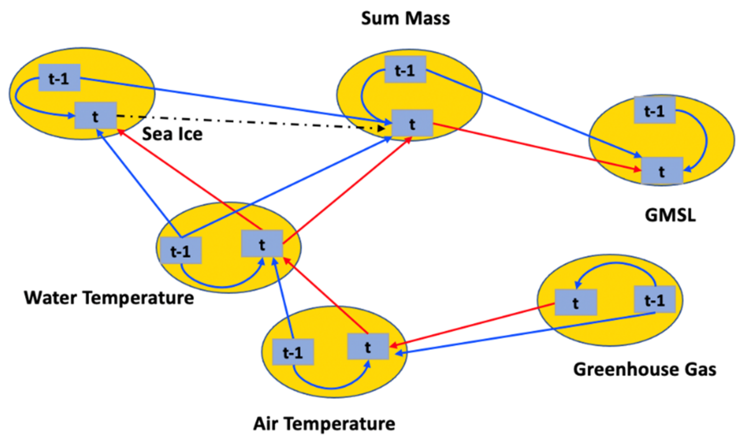
After the data transformation, the dynamic VAR(1)-SEM can be analyzed by the usual SEM software as we have shown previously [21]. In this work, the SEM software adopted is the Lavaan package in R. Confirmed pathways are depicted in Figure 6 below, with the estimated path coefficients and other statistics tabulated in Table 2. In summary, we found that nearly all the contemporaneous pathways were significant except for the pathway between Sea Ice(t) and Sum Mass(t). The data validated a significant pathway from Greenhouse Gas increase to Air Temperature increase, to Water Temperature increase, to Sea Ice Extent, to Sum Mass (glaciers cumulative mass loss), and subsequently, to Global Mean Sea-level rise.
Table 2 shows the estimates of the parameters in the VAR(1)-SEM model. The RMSEA of this model is 0.400. The Mean in this table is the mean slope across the multiple imputation samples. After we drop the non-significant pathway at the significance level of 0.05 (2-sided), the resulting validated VAR (1)-SEM model is represented by the following equation system:
G M S L t = 9.182 × S u m   M a s s t 10.005 × S u m   M a s s t 1 + 0.983 × G M S L t 1 + 7.315 , S u m   M . t = 0.019 × W a t e r   T . t 0.024 × W a t e r   T . t 1 0.005 × S e a   I c e t 1 + 1.034 × S u m   M a s s   t 1 0.163 , S e a   I c e t = 0.802 × W a t e r   T . t 0.466 × W a t e r   T . t 1 + 0.646 × S e a   I c e t 1 + 23.307 , W a t e r   T . t = 0.951 × A i r   T . t 0.447 × A i r   T . t + 0.447 × W a t e r   T . t 1 + 1.011 , A i r   T . t = 0.118 × G r e e n h o u s e t + 0.123 × G r e e n h o u s e t + 0.755 × A i r   T . t 1 + 1.655 , G r e e n h o u s e t = 0.979 × G r e e n h o u s e t 1 + 8.108 .

3.2. GMSL Projection with VAR(3)

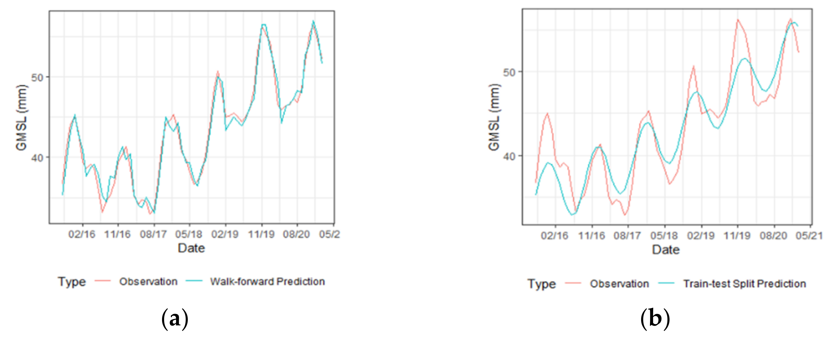
Using significant variables and pathways confirmed by the dynamic SEM analysis, we have subsequently selected monthly Average Sea Ice Extent, Water Temperature, the sum of Antarctic and Greenland Ice Sheet mass, in addition to GMSL, for the ensuing refined VAR analysis. Although Air Temperature is also significant, it is highly correlated to Water Temperature, and was thus discarded to avoid multicollinearity. The optimal number of lags is determined by using the Bayesian Information Criterion (BIC). This analysis resulted in the optimal number of lags being 3, and thus the VAR(3) model is fitted subsequently. The Multiple R2 for GMSL is 0.997. To validate the superiority of the VAR(3) model, we have also compared it to the best baseline ARIMA model, the ARIMA(2,1,2) as selected by BIC. We applied Root Mean Square Error (RMSE) and Mean Absolute Error (MAE) to compare the predicting performance of these two models. Both statistics are used for measuring the discrepancy between predicted and observed values, and thus a smaller value indicates better performance. These results are shown in Figure 7 and Table 3. One can find that the predicting accuracy is improved by using VAR(3) than the ARIMA(2,1,2) according to both RMSE and MAE.
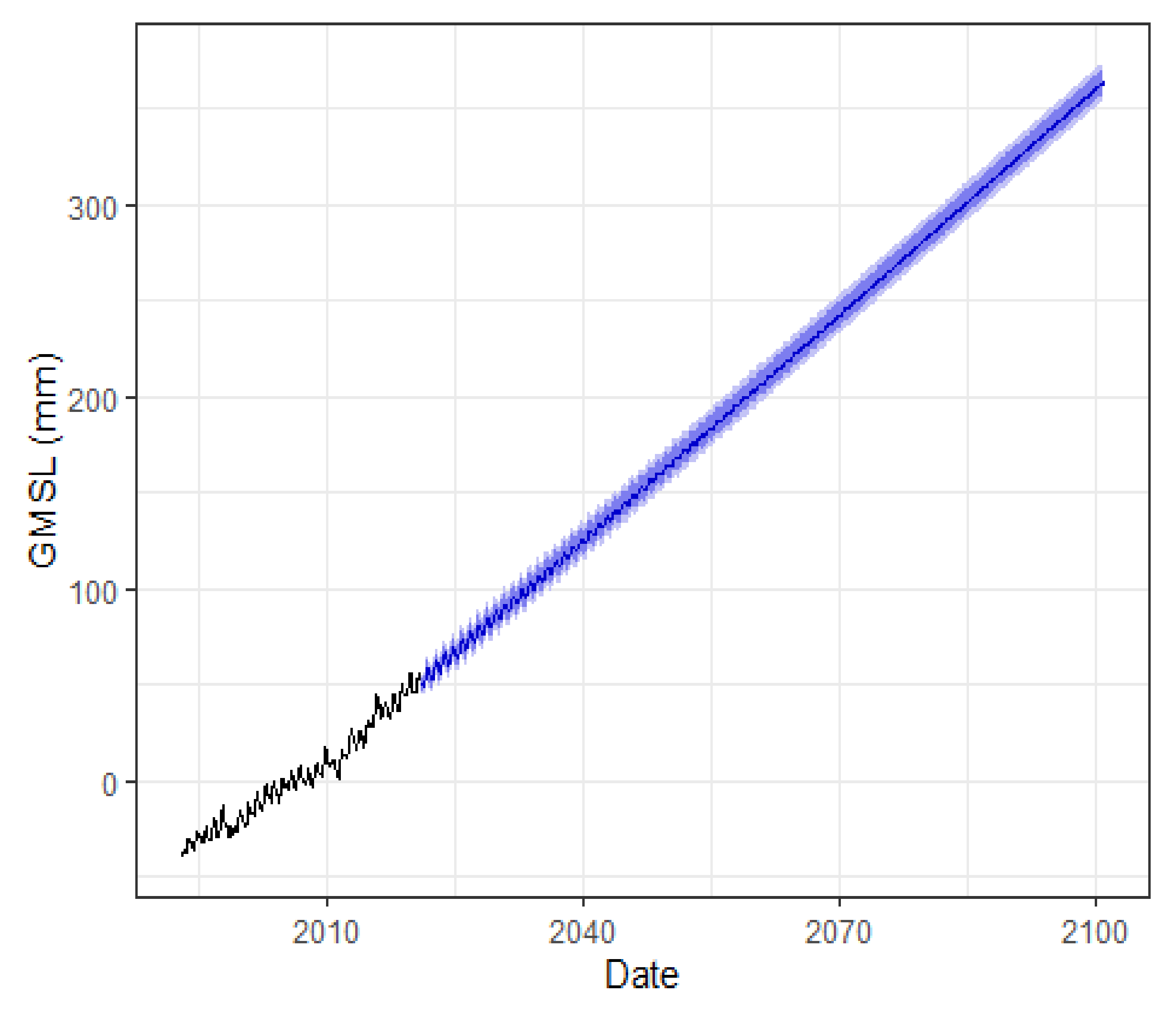
After validating the model, we reconstructed the VAR(3) model by applying all observed data available to date, from January 1993 to May 2021, and forecasted the global mean sea level for the next 80 years (see Figure 8). The expected mean global sea level change is 0.31 m by the end of the 21st century. However, to ensure statistical confidence and to guard against the worst-case scenarios, we used an upper bound of the 95% prediction interval for the ensuing forecast.
The relevant equation used to predict GMSL by the VAR(3) model is shown below:
G M S L t = 1.398 × G M S L t 1 0.010 × W a t e r   T . t 1 0.018 × S u m   M a s s t 1 0.702 × S e a   I c e t 1 0.835 × G M S L t 2 + 0.150 × W a t e r   T . t 2 + 0.044   × S u m   M a s s t 2 + 0.894 × S e a   I c e t 2 + 0.359 × G M S L t 3 + 0.403 × W a t e r   T . t 3 0.026 × S u m   M a s s t 3 0.220 × S e a   I c e t 3 + 0.013 × t 10.339

3.3. Projections of Coastal Regional Sea-Level Rise with GAM

We analyzed regional tidal gauges located in areas of New York City and Long Island, Miami, and New Orleans. Using the generalized additive model (GAM), we modeled the relations between Global Mean Sea Level and Regional Sea Level (RSL). The RSL data for each region of interest are obtained by averaging the observed RSL from multiple regional tidal gauge stations. For instance, the RSL of New York City and Long Island is obtained from the Montauk, Kings Point, Battery Park, and Bergen Point tidal gauge stations. The related path diagram for this GAM analysis is shown in Figure 9.
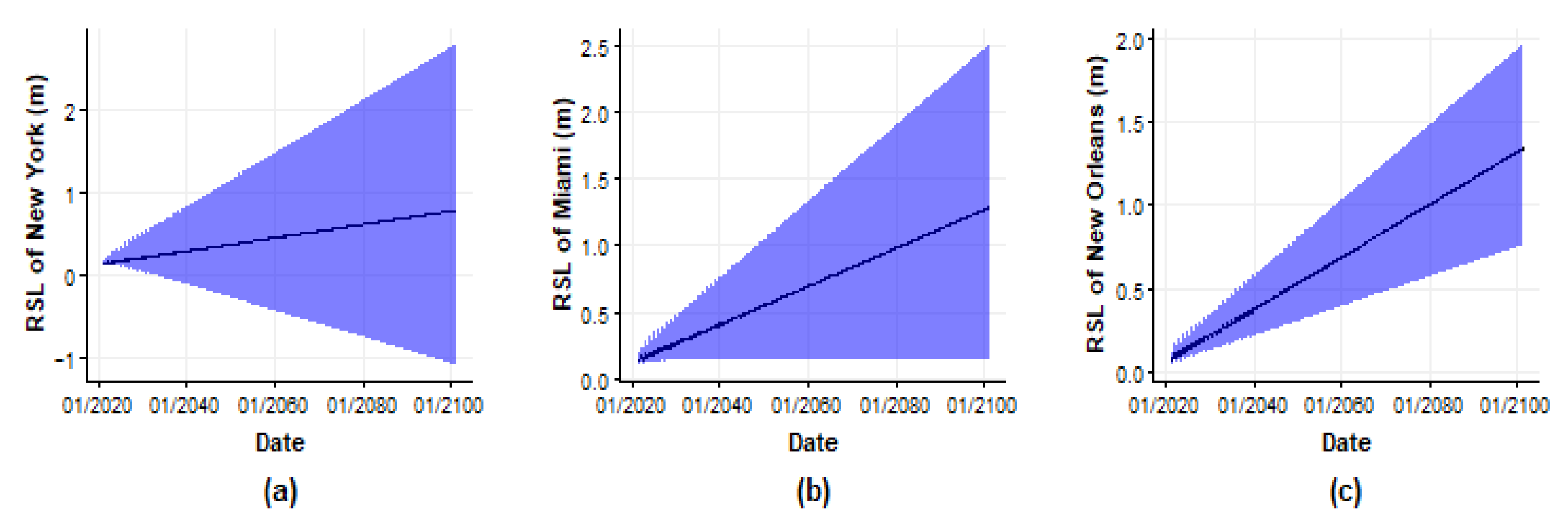
According to the results from the GAM model, the expected RSL rise for the New York City and the Long Island area is approximately 0.24 m by 2050 and 0.65 m by 2100. The prediction intervals show the likely RSL rise can range from −0.43 to 1.04 m by the end of 2050 and from −1.22 to 2.63 m by the end of 2100. The performance of linear regression and GAM were compared, and we found that the adjusted R 2 improved by 0.083, and the deviance explained improved by 0.098 using GAM with its adjusted R 2 being 0.348. One may notice that the prediction bands would rise over time. This is due to two main reasons: (1) The increased variability of RSL as time increases, which subsequently increased the prediction temporal volatility of GAM; (2) To calculate the prediction bands, we first use the upper bounds and lower bounds of the 95% prediction intervals for GMSL from the VAR(3) predictions as our predictor. Using the upper bounds of the VAR(3) and then GAM prediction bands, we can predict the worst-case scenario for coastal flooding, which is defined at a certain threshold above normal sea level. According to NOAA, the threshold for major flooding scale is 1.17 m (±0.39) above the local diurnal tidal range [4]. Therefore, we can approximate the worst-case scenario for flooding for the New York City and Long Island region to be 1.17 m + 0.39 m + 1.04 m = 2.6 m by 2050 and 1.17 m + 0.39 m + 2.63 m = 4.19 m by 2100. The results for other locations are similar as shown below.
The expected RSL rise for Miami is approximately 0.49 m by the end of 2050 and 1.21 m by the end of 2100. The prediction intervals show the likely RSL rise can range from 0.06 to 0.99 m by the end of 2050 and from 0.07 to 2.42 m by the end of 2100. After replacing the linear regression with a GAM, the adjusted R 2 improved by 0.123, and the deviance explained improved by 0.13. Its adjusted R 2 is 0.388. Using NOAA’s major flooding threshold, we can approximate the worst-case scenario for flooding for Miami to be 1.17 m + 0.39 m + 0.99 m = 2.55 m by 2050 and 1.17 m + 0.39 m + 2.42 m = 3.98 m by 2100.
The expected RSL rise for New Orleans is 0.58 m by the end of 2050 and 1.37 m by the end of 2100. The prediction intervals show the likely RSL rise can range from 0.34 to 0.85 m by the end of 2050 and from 0.78 to 1.98 m by the end of 2100. After replacing the linear regression with a GAM, the adjusted R 2 improved by 0.418, and the deviance explained improved by 0.418. Its adjusted R 2 is 0.683. Using NOAA’s major flooding threshold, we can approximate the worst-case scenario for flooding for New Orleans to be 1.17 m + 0.39 m + 0.85 m = 2.41 m by 2050 and 1.17 m + 0.39 m + 1.98 m = 3.54 m by 2100. The RSL projections for each of the three regions of interest are shown in Figure 10.
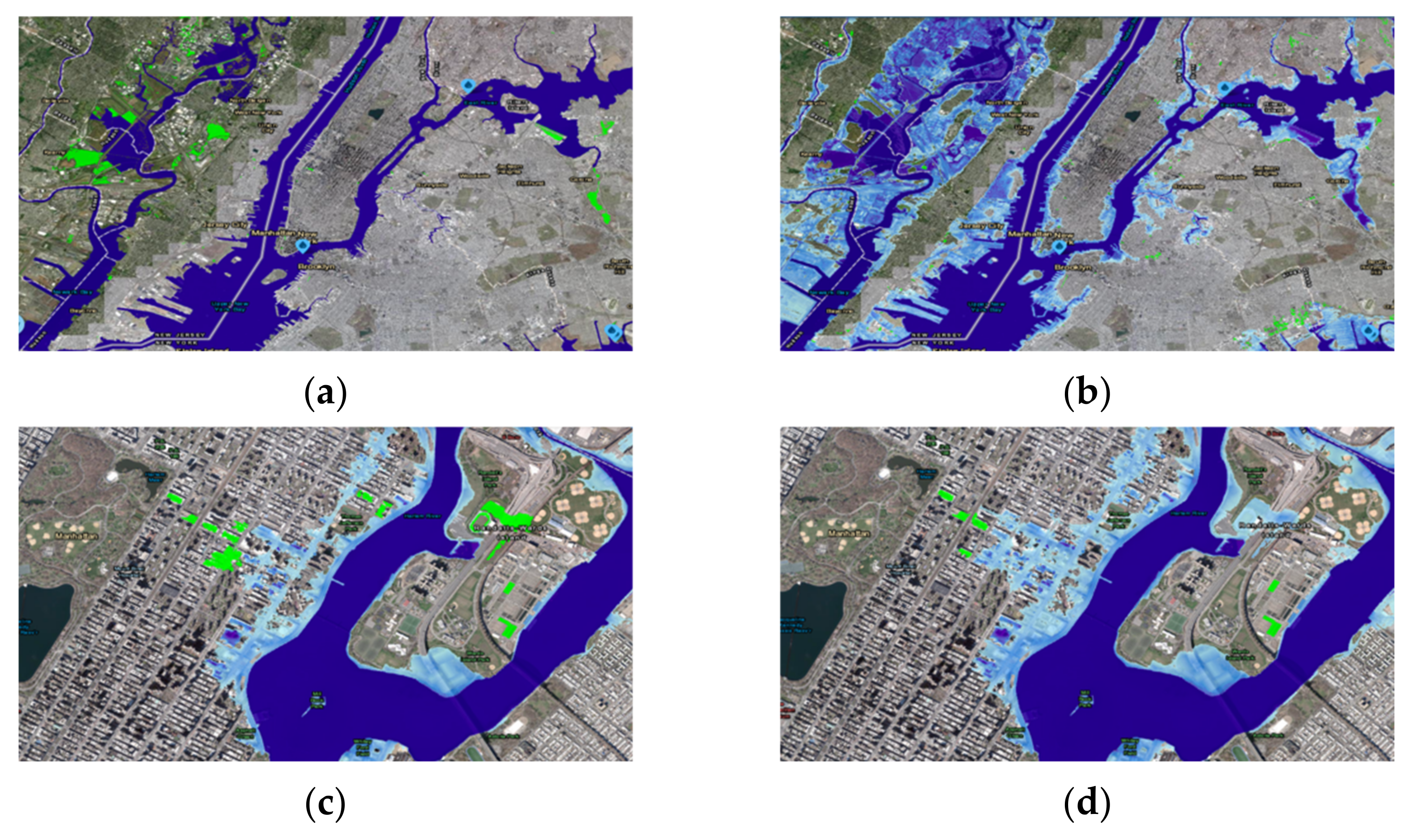
Using the NOAA Sea-level rise Viewer [29], we plotted the respective coastal inundation scenarios for 2050 and 2100, respectively, in New York City, Miami, and New Orleans (see Figure 11, Figure 12 and Figure 13).

4. Discussion

Using the dynamic VAR(1)-SEM Model based on an existing public database, we have confirmed a significant pathway, from rising levels of greenhouse gases, to air temperature increase, to sea water temperature increase, to sea ice extent, to land ice (glaciers) mass loss, and subsequently, to global sea-level rise. As expected, greenhouse gases were a significant predictor of air temperature and global mean sea-level rise. In contrast, a controversial discovery was that the sea ice turned out to be critical in keeping the effects of the dynamic SEM Model. This could be due to a number of reasons. Firstly, declining sea ice means that there is less white surface to reflect the incoming sunlight, which lowers the albedo and thus leads to greater absorption and warming in the atmosphere, increasing the melting of sea and land ice [30]. Secondly, sea ice is also integral to ocean circulation, as the brine rejection below the sea ice increases the density of the water, causing it to sink and contribute to the global ocean conveyor belt [30].
The VAR(3) model took up the three significant and most direct factors for global sea-level rise from the dynamic SEM analysis. By using the optimal number of predictive lags in time, which was found to be 3, the VAR(3) model rendered more refined forecasting of sea level for the next 80 years, projecting a global mean sea-level rise of approximately 0.31 m by 2100. The GAM, which was found to be superior to the linear regression, was able to link GMSL and RSL for three regions of interest: New York City and Long Island, Miami, and New Orleans. The respective regional coastal sea-level rise projections were 0.65 m for New York City and Long Island, 1.21 m for Miami, and 1.37 m for New Orleans by 2100. Furthermore, the worst-case scenarios for flooding are projected to be 2.6 m by 2050 and 4.19 m by 2100, for New York City and Long Island; 2.55 m by 2050 and 3.98 m by 2100, for Miami; 2.41 m by 2050 and 3.54 m by 2100, for New Orleans.
Regional differences in elevation, ocean circulation, and coastal topography could account for the differences in sea-level projections. When considering the increased scope and severity of tidal flooding from sea-level rise, it is essential to factor in the thresholds for major flooding scenarios. Decades ago, typically only powerful storms could cause coastal flooding; however, due to regional sea-level rise, rather common wind events and seasonally high tides are now often the main cause of coastal inundation in communities [31], indicating that such events will persist and even worsen in future decades. Based on the NOAA’s major flooding threshold, our new RSL predictions, when analyzed in coastal regions, show extensive flooding inland. Notably, flooding in Manhattan can be observed reaching deep inland in the Central Park region, along with significant inundation along the coast of Florida.
As a major objective of our analysis, we wish to develop a sensible open-box analysis pipeline using publicly available data for sea-level rise prediction. We have found that our predictions are aligned with major climate models from public agencies such as the IPCC, which reports an estimated sea-level rise between 0.43 m (0.29–0.59 m) and 0.84 m (0.61–1.10 m) [3]. This has convinced us that climate change and sea-level rise are not fiction nor conspiracy. As temperature increases and climate change progressively worsens, causing sea-level rise and extreme tidal flooding, millions of lives, property value, and ecosystems are at stake. Potential impacts of recurrent coastal flooding extend beyond sea-level rise. Examples include infiltration and degradation of stormwater and wastewater systems, and saltwater intrusion that raises coastal groundwater tables [32]. Potential responses for prevention measures could include building protective barriers, especially in urban areas such as New York City, where infrastructure such as subways is unprepared for the increased amount and severity of flooding, as evidenced by Hurricane Elsa in July 2021 [33]. Additionally, we hope our analyses encourages the protection of communities that are disproportionately impacted by coastal flooding and are the most vulnerable to socioeconomic damage. Developing sustainable technology and good management of coastal communities is also essential. However, identifying the most appropriate way to respond to sea-level rise is not straightforward and is contested with a range of governance challenges. Finding an ideal response to sea-level rise requires an assessment of their relative effectiveness, technical limits, costs, drawbacks, and the specific governance challenges associated with each type of response. Through our analysis, we hope to directly impact public policy and opinion for the environmental protection of coastal properties and proactive preparation from the impending climate crisis on the effects of sea-level rise on communities.
Lastly, we acknowledge that our work is not without limitations. Even with our model, it still remains a complex issue involving many other variables such as isostatic adjustment, wind forcing, sea level pressure, or climatic periodicities. Additionally, to account for the relatively low adjusted R 2 values for the GAM model, our confidence intervals became much larger over time due to large noise in the dataset. Lastly, as the data for the Greenland and Antarctic ice masses were only accessible from 1992, and as it is critical to consider the proportions of missing data compared to the available dataset when utilizing imputation, our ability to create more accurate forecasting of sea-level rise was limited. As the concluding remark for our work, we call for public agencies to provide more comprehensive data sets for citizen scientists in order to be able to independently model, analyze, and thus verify critical claims on the ongoing climate crisis.

Author Contributions

Conceptualization, W.Z. and J.C. (Jean Chung); Data Curation, J.C. (Jean Chung), J.C. (Jiayou Chao) and G.T.; Methodology, J.C. (Jiayou Chao), J.C. (Jean Chung), G.T. and W.Z.; Software, J.C. (Jiayou Chao), J.C. (Jean Chung) and G.T.; Validation, J.C. (Jiayou Chao), J.C. (Jean Chung), G.T. and W.Z.; Formal Analysis, J.C. (Jiayou Chao), J.C. (Jean Chung) and G.T.; Investigation, J.C. (Jiayou Chao), J.C, (Jean Chung), G.T. and W.Z.; Resources, J.C. (Jiayou Chao), J.C. (Jean Chung), G.T. and W.Z.; Data Curation, J.C. (Jiayou Chao), J.C. (Jean Chung) and G.T.; Writing—Original Draft Preparation, J.C. (Jiayou Chao), J.C. (Jean Chung), G.T. and W.Z.; Writing—Review & Editing, J.C. (Jiayou Chao), J.C. (Jean Chung), G.T. and W.Z.; Visualization, J.C. (Jiayou Chao), J.C. (Jean Chung), G.T. and W.Z.; Supervision, W.Z. All authors have read and agreed to the published version of the manuscript.

Funding

This research received no external funding.

Institutional Review Board Statement

Not applicable.

Informed Consent Statement

Not applicable.

Data Availability

The CO2 data analyzed in this study are openly available in Scripps CO2 Program at https://scrippsco2.ucsd.edu/data/atmospheric_co2/primary_mlo_co2_record.html, (accessed on 8 October 2021), reference number [16]. The CH4 and N2O data analyzed in this study are openly available at the 2degreesinstitute: https://www.2degreesinstitute.org, (accessed on 8 October 2021), reference number [17]. The Sea Level data analyzed in this study are openly available in the NASA Sea Level Change Program at https://climate.nasa.gov/vital-signs/sea-level/, (accessed on 8 October 2021), reference number [11]. The Greenland Ice Sheet and Antarctic Ice Sheet cumulative ice mass data analyzed in this study are openly available in IMBIE at http://imbie.org/data-downloads/, (accessed on 8 September 2021), reference number [13], and in NASA at https://climate.nasa.gov/vital-signs/ice-sheets/, (accessed on 20 November 2021), reference number [14]. The monthly sea ice average extent and area analyzed in this study are openly available at NSIDC at https://nsidc.org/arcticseaicenews/sea-ice-tools/, (accessed on 8 October 2021), reference number [12]. The monthly air and water temperatures analyzed in this study are openly available at Berkeley Earth at https://doi.org/10.5194/essd-12-3469-2020, (accessed on 8 October 2021, reference number [15]. The regional coastal tide gauge data analyzed in this study are openly available at the NOAA Center for Operational Oceanographic Products and Services at https://tidesandcurrents.noaa.gov/sltrends/sltrends_global.html, (accessed on 8 October 2021), reference number [18].

Conflicts of Interest

The authors declare no conflict of interest.

References

  1. Climate.gov. Available online: https://www.climate.gov/news-features/understanding-climate/climate-change-global-sea-level (accessed on 8 October 2021).
  2. Schmith, T.; Johansen, S.; Thejll, P. Statistical analysis of global surface temperature and sea level using cointegration methods. J. Clim. 2012, 25, 7822–7833. [Google Scholar] [CrossRef]
  3. Oppenheimer, M.; Glavovic, B.; Hinkel, J.; van de Wal, R.; Magnan, A.K.; Abd-Elgawad, A.; Cai, R.; Cifuentes-Jara, M.; Deconto, R.M.; Ghosh, T.; et al. Sea Level Rise and Implications for Low Lying Islands, Coasts and Communities; The Intergovernmental Panel on Climate Change: Geneva, Switzerland, 2019. [Google Scholar]
  4. Sweet, W.W.V.; Dusek, G.; Obeysekera, J.T.B.; Marra, J.J. Patterns and Projections of High Tide Flooding along the US Coastline Using a Common Impact Threshold; NASA Technical Report NOS CO-OPS; National Oceanic and Atmospheric Administration: Washington, DC, USA, 2018. [Google Scholar]
  5. NPR. Available online: https://www.npr.org/templates/story/story.php?storyId=9162438#:~:text=Study%3A%20634%20Million%20People%20at%20Risk%20from%20Rising%20Seas%20A,related%20impacts%20of%20climate%20change (accessed on 8 October 2021).
  6. Balogun, A.-L.; Adebisi, N. Sea level prediction using ARIMA, SVR and LSTM neural network: Assessing the impact of ensemble Ocean-Atmospheric processes on models’ accuracy. Geomat. Nat. Hazards Risk 2021, 12, 653–674. [Google Scholar] [CrossRef]
  7. Johansen, S. The Analysis of Nonstationary Time Series Using Regression, Correlation and Cointegration with an Application to Annual mean Temperature and Sea Level; University of Copenhagen Department of Economics Discussion Papers No. 10–27; University of Copenhagen, Department of Economics: Copenhagen, Denmark, 2010. [Google Scholar]
  8. Aral, M.M.; Guan, J.; Chang, B. Dynamic system model to predict global sea-level rise and temperature change. J. Hydrol. Eng. 2012, 17, 237–242. [Google Scholar] [CrossRef]
  9. Aral, M.M.; Guan, J. Global sea surface temperature and sea level rise estimation with optimal historical time lag data. Water 2016, 8, 519. [Google Scholar] [CrossRef] [Green Version]
  10. Bâki İz, H.; Shum, C.K. Recent and future manifestations of a contingent global mean sea level acceleration. J. Geod. Sci. 2020, 10, 153–162. [Google Scholar]
  11. Beckley, B.; Zelensky, N.P.; Holmes, S.A.; Lemoine, F.G.; Ray, R.D.; Mitchum, G.T.; Desai, S.; Brown, S.T. Global Mean Sea Level Trend from Integrated Multi-Mission Ocean Altimeters TOPEX/Poseidon Jason-1 and OSTM/Jason-2 Version 4.2; NASA Physical Oceanography Distributed Active Archive Center: Pasadena, CA, USA, 2016. [Google Scholar]
  12. Sea Ice Data and Analysis Tools|Arctic Sea Ice News and Analysis. Available online: https://nsidc.org/arcticseaicenews/sea-ice-tools/ (accessed on 8 October 2021).
  13. IMBIE (Ice Sheet Mass Balance Inter-comparison Exercise). Available online: http://imbie.org/data-downloads/ (accessed on 8 September 2021).
  14. NASA (Ice Sheet. NASA). Available online: https://climate.nasa.gov/vital-signs/ice-sheets/ (accessed on 20 November 2021).
  15. Rohde, R.A.; Hausfather, Z. The Berkeley Earth land/ocean temperature record. Earth Syst. Sci. Data 2020, 12, 3469–3479. [Google Scholar] [CrossRef]
  16. Keeling, C.D.; Piper, S.C.; Bacastow, R.B.; Wahlen, M.; Whorf, T.P.; Heimann, M.; Meijer, H.A. Exchanges of Atmospheric CO2 and 13CO2 with the Terrestrial Biosphere and Oceans from 1978 to 2000. I. Global Aspects; Scripps Institution of Oceanography: San Diego, CA, USA, 2001. [Google Scholar]
  17. 2degreesinstitute. Available online: https://www.2degreesinstitute.org (accessed on 8 October 2021).
  18. NOAA Center for Operational Oceanographic Products and Services. Available online: https://tidesandcurrents.noaa.gov/sltrends/sltrends_global.html (accessed on 8 October 2021).
  19. Kline, R.B. Principles and Practice of Structural Equation Modeling; Guilford Publications: New York, NY, USA, 2015. [Google Scholar]
  20. Schumacker, R.E.; Lomax, R. A Beginner’s Guide to Structural Equation Modeling; Lawrence Erlbaum Associates: New Jersey, NJ, USA, 2004. [Google Scholar]
  21. Byrne, B.M. Structural Equation Modeling with Mplus: Basic Concepts, Applications, and Programming; Routledge: Oxfordshire, UK, 2013. [Google Scholar]
  22. Kim, J.; Zhu, W.; Chang, L.; Bentler, P.M.; Ernst, T. Unified structural equation modeling approach for the analysis of multisubject, multivariate functional MRI data. Hum. Brain Mapp. 2007, 28, 85–93. [Google Scholar] [CrossRef] [PubMed]
  23. Di Narzo, A.F.; Aznarte, J.L.; Stigler, M.; Tsung-wu, H. tsDyn: Nonlinear Time Series Models with Regime Switching; R Package Version 10-1.2; R Foundation for Statistical Computing: Vienna, Austria, 2020; Available online: https://www.r-project.org (accessed on 1 December 2021).
  24. Pfaff, B.; Stigler, M. Vars: VAR Modelling; R Package Version 1.5-3; R Foundation for Statistical Computing: Vienna, Austria, 2018. [Google Scholar]
  25. MultiThreaded. Available online: https://multithreaded.stitchfix.com/blog/2015/07/30/gam/ (accessed on 8 October 2021).
  26. Wood, S. Mixed GAM Computation Vehicle with Automatic Smoothness Estimation; R Package Version 1.8-35; R Foundation for Statistical Computing: Vienna, Austria, 2021. [Google Scholar]
  27. Wood, S.N. Stable and efficient multiple smoothing parameter estimation for generalized additive models. J. Am. Stat. Assoc. 2004, 99, 673–686. [Google Scholar] [CrossRef] [Green Version]
  28. Wood, S.N. Fast stable restricted maximum likelihood and marginal likelihood estimation of semiparametric generalized linear models. J. R. Stat. Soc. Ser. B (Stat. Methodol.) 2011, 73, 3–36. [Google Scholar] [CrossRef] [Green Version]
  29. Marcy, D.; Brooks, W.; Draganov, K.; Hadley, B.; Haynes, C.; Herold, N.; McCombs, J.; Pendleton, M.; Ryan, S.; Schmid, K.; et al. New mapping tool and techniques for visualizing sea level rise and coastal flooding impacts. Solut. Coast. Disasters 2011, 2011, 474–490. [Google Scholar]
  30. National Oceanic and Atmospheric Administration U.S. Department of Commerce. Available online: https://oceanservice.noaa.gov/facts/sea-ice-climate.html (accessed on 8 October 2021).
  31. Sweet, W.; Park, J.; Marra, J.; Zervas, C.; Gill, S. Sea Level Rise and Nuisance Flood Frequency Changes around the United States; NOAA Technical Report NOS CO-OPS; National Oceanic and Atmospheric Administration: Washington, DC, USA, 2014. [Google Scholar]
  32. Sukop, M.C.; Rogers, M.; Guannel, G.; Infanti, J.M.; Hagemann, K. High temporal resolution modeling of the impact of rain, tides, and sea level rise on water table flooding in the Arch Creek basin, Miami-Dade County Florida USA. Sci. Total Environ. 2018, 616–617, 1668–1688. [Google Scholar] [CrossRef] [PubMed]
  33. New York Times. Available online: https://www.nytimes.com/2021/07/07/us/tropical-storm-elsa-florida.html (accessed on 9 October 2021).
Figure 1. (a) Condominium collapse in Miami due to flooding (Courtesy of: Miami Herald); (b) Subway/streets flooding in New York City due to Hurricane Ida (Courtesy of: New York Post); (c) New Orleans flash flood (Courtesy of: Washington Post).
Stats 05 00002 g001
Figure 2. The proposed sea-level change analysis pipeline with three sequential steps: (1) a dynamic Structural Equation Model (SEM) to identify pathways between the global mean sea level (GMSL) and various predictors, (2) a Vector Autoregression Model (VAR) to quantify the GMSL changes due to the significant relations identified in the first step, and (3) a Generalized Additive Model (GAM) to model the relationship between regional sea level (RSL) and GMSL.
Stats 05 00002 g002
Figure 3. Hypothesized path diagram for the dynamic structural equation [VAR(1)-SEM] model. Here, red lines represent contemporaneous relationships while blue lines represent longitudinal relationships. ‘GMSL’ represents the monthly global mean sea level. ‘Sum Mass’ represents the combined Greenland and Antarctic (land) Ice Sheet monthly mass losses. ‘Sea Ice’ refers to the monthly average sea ice extent in the Northern Hemisphere. See Table 1 for more variable definitions.
Stats 05 00002 g003
Figure 4. Path diagram for VAR(3) with GMSL being the response variable and three predictors selected from the dynamic SEM step.
Stats 05 00002 g004
Figure 5. Pathway diagram of the Generalized Additive Model (GAM) to model the relationship between GMSL to RSL (Regional Sea Level) via select tidal gauges near each region of interest (e.g., NYC and Long Island, Miami, New Orleans).
Stats 05 00002 g005
Figure 6. Dynamic VAR(1)-SEM Results: The dashed lines indicate pathways that were not significant. Solid blue lines indicate a significant longitudinal path from t − 1 to t, while solid red lines indicate a significant contemporaneous path from t to t.
Stats 05 00002 g006
Figure 7. (a) Predicted numerical results for walk-forward validation method by VAR(3); (b) Predicted numerical results for train-test split validation method by VAR(3).
Stats 05 00002 g007
Figure 8. GMSL from 2021 to 2100 predicted by the VAR(3) model using the observed data (January 1993–May 2021) with the 80% (darker blue area) and the 95% (lighter blue area) prediction interval bands.
Stats 05 00002 g008
Figure 9. Pathway diagram of the Generalized Additive Model (GAM) to model the relationship between GMSL to RSL (Regional Sea Level) via four regional tidal gauge stations in the New York City and Long Island area.
Stats 05 00002 g009
Figure 10. The blue area represents the prediction intervals. (a) Predicted regional sea levels of New York City; (b) Miami and (c) New Orleans over the next 80 years.
Stats 05 00002 g010
Figure 11. Light blue regions indicate areas of sea-level inundation. (a) New York City and vicinity with sea level in 2021; (b) and the extent of extreme flooding due to sea-level rise by 2100; (c) show significant flooding pictured in the Central Park region of Manhattan, New York by 2050 and (d) 2100.
Stats 05 00002 g011
Figure 12. (a) Here we show sea level at the present day (2021); (b) predicted extreme flooding by 2050 and (c) 2100 in Miami, Florida, and surrounding cities.
Stats 05 00002 g012
Figure 13. Here we show sea level (a) in 2021; (b) and predicted extreme flooding by 2050; (c) and 2100 in New Orleans, Louisiana and vicinity.
Stats 05 00002 g013
Table 1. Definition of global variables used in the proposed analysis pipeline. The only variable not included are regional sea levels measured by various regional tidal gauge stations.
VariableExplanation
Air TemperatureGlobal average air temperature
GMSLGlobal mean sea-level variation
Sum MassSummation of Greenland and Antarctic cumulative glacier mass change
Greenhouse GasThe amount of CO2, N2O and CH4 in the air (parts per million)
Water TemperatureGlobal average water temperature
Sea IceNorthern hemisphere sea ice extent
Table 2. VAR(1)-SEM Results.
Significant Path ConnectionMean (SE)t-Value (p-Value, 2-Sided)
Sum Mass(t) → GMSL(t)9.366 (4.528)2.068 (0.039)
Sum Mass(t − 1) → GMSL(t)−10.242 (4.714)−2.173 (0.030)
GMSL(t − 1) → GMSL(t)0.979 (0.009)107.188 (0.000)
Sum Mass(t − 1) → Sum M.(t) 1.034 (0.001)817.450 (0.000)
Water T.(t) → Sum M.(t) 0.021 (0.002)8.305 (0.000)
Water T.(t − 1) → Sum M.(t) −0.024 (0.002)−13.721 (0.000)
Sea Ice(t) → Sum M.(t) 0.002 (0.002)0.944 (0.345)
Sea Ice(t − 1) → Sum M.(t) −0.006 (0.001)−4.727 (0.000)
Sea Ice(t − 1) → Sea Ice(t)0.697 (0.013)52.521 (0.000)
Water T.(t)→ Sea Ice(t)−1.098 (0.052)−20.924 (0.000)
Water T.(t − 1) → Sea Ice(t)−0.328 (0.053)−6.202 (0.000)
Air T.(t) → Water T.(t)0.951 (0.005)203.096 (0.000)
Air T.(t − 1) → Water T.(t)−0.447 (0.040)−11.039 (0.000)
Water T.(t − 1) → Water T.(t)0.447 (0.043)10.324 (0.000)
Greenhouse(t) → Air T.(t)−0.118 (0.007)−16.941 (0.000)
Greenhouse(t) → Air T.(t)0.123 (0.007)17.625 (0.000)
Air T.(t − 1) → Air T.(t)0.755 (0.020)37.435 (0.000)
Greenhouse(t − 1) → Greenhouse(t)0.979 (0.012)82.789 (0.000)
Table 3. Comparison of predicting performance between VAR(3) and ARIMA(2,1,2).
MethodModelRMSEMAE
Walk-forwardARIMA(2,1,2)1.441.21
Walk-forwardVAR(3)1.070.89
Train-test splitARIMA(2,1,2)6.675.55
Train-test splitVAR(3)2.482.02
Publisher’s Note: MDPI stays neutral with regard to jurisdictional claims in published maps and institutional affiliations.