Article

Multiple Imputation of Composite Covariates in Survival Studies

1
School of Mathematical Sciences, University of Southampton, Southampton SO17 1BJ, UK
2
School of Mathematics and Statistics, The Open University, Milton Keynes MK7 6AA, UK
*
Author to whom correspondence should be addressed.
Stats 2022, 5(2), 358-370; https://doi.org/10.3390/stats5020020
Submission received: 4 February 2022 / Revised: 11 March 2022 / Accepted: 15 March 2022 / Published: 29 March 2022
(This article belongs to the Special Issue Survival Analysis: Models and Applications)

Abstract

:
Missing covariate values are a common problem in survival studies, and the method of choice when handling such incomplete data is often multiple imputation. However, it is not obvious how this can be used most effectively when an incomplete covariate is a function of other covariates. For example, body mass index (BMI) is the ratio of weight and height-squared. In this situation, the following question arises: Should a composite covariate such as BMI be imputed directly, or is it advantageous to impute its constituents, weight and height, first and to construct BMI afterwards? We address this question through a carefully designed simulation study that compares various approaches to multiple imputation of composite covariates in a survival context. We discuss advantages and limitations of these approaches for various types of missingness and imputation models. Our results are a first step towards providing much needed guidance to practitioners for analysing their incomplete survival data effectively.

1. Introduction

A problem faced by analysts in survival studies is the ubiquity of missing covariate values. If not handled appropriately, the effects can be wide ranging and the loss of data can lead to inefficiencies and introduce bias into analyses. A widely used approach to analyse incomplete data sets is multiple imputation (MI), introduced in [1]. However, there are situations where it is not obvious how this can be used most effectively.
A motivating data set for our research was supplied by NHS Blood and Transplant and is a rather typical routinely collected survival data set. It involves censored survival times for 7732 kidney transplant patients and contains information on 30 covariates thought to be potentially related to post-transplant survival. Full details are given in [2]. Whilst there are relatively few missing values for most of these covariates, one, Body Mass Index (BMI) of the kidney donor has over 60 per cent of values missing. BMI is defined as the ratio of an individual’s weight in kilograms to the square of the height in metres:
B M I = w e i g h t ( kg ) / h e i g h t ( m ) 2 .
This is an example of a composite covariate: it is a function of two constituents, namely weight and height in this case. In [2] the authors investigate whether MI is an appropriate approach for dealing with such a high proportion of missing values in the context of survival analysis and show that MI outperforms listwise deletion of observations with at least one missing covariate (complete case analysis). However, they do not use the composite nature of BMI explicitly in their analysis.
There are several possible approaches to imputing a composite covariate. The two main ones are active imputation and passive imputation. In active imputation, also called “Just another variable”, the composite covariate is imputed directly like any other variable. As a result, the functional relationship between the imputed composite covariate and its constituents is diminished. This is the approach used in [2]. In passive imputation, the constituents are imputed and the composite covariate is only then constructed. Hence the functional relationship is preserved in passive imputation. However, the relationship between the composite covariate and other variables in the data set, such as the outcome variable, can be underestimated since the other variables do not directly influence the imputation of the composite covariate.
To combat this issue with passive imputation, a modification called Substantive Model Compatible Fully Conditional Specification (SMCFCS) has been proposed; see, for example [3,4]. In SMCFCS the outcome variable is accounted for when imputing the composite covariate in order to preserve the relationship between the composite covariate and the outcome variable.
MI for composite covariates in a survival analysis context has not been widely explored in the literature, so our aim is to make a start to filling this gap. We will investigate the performance of active and passive imputation for survival data via a simulation study, the design for which has been informed by the motivating data set.
In Section 2, we first introduce some background on missing data mechanisms and MI before describing the design of our simulation study and giving some criteria for comparing the performance of active and passive imputation. In particular, we introduce the variants of MI to be considered in our study and investigate how the missing data mechanism and the presence of further covariates - beyond the composite covariate and its constituents—will affect the performance of the different MI methods. The results are given in Section 3, and their implications are further discussed in Section 4.

2. Background and Methods

In this section, we first outline different missingness mechanisms since these may have an impact on the performance of MI. Following this is a brief overview of the general concept of MI. We then introduce more specific methods relating to MI, such as Fully Conditional Specification (FCS) and variants of active and passive imputation. Finally, we provide the design of our simulation study, with details of the process to generate the data, to set missing values, and the models to impute the missing values.

2.1. Missingness Mechanisms

Assume a n × p data set with n observations and p covariates. Denote this data set by X = ( x 1 , . . . , x p ) where x j = ( x 1 j , . . . , x n j ) for the j th covariate, j = 1 , . . . , p . For each x i j , denote a missingness indicator, r i j , where r i j = 1 if x i j is observed, and r i j = 0 otherwise. These values build a missingness matrix R = ( r 1 , . . . , r p ) where r j = ( r 1 j , . . . , r n j ) . X can be decomposed into a missing part, X M , and an observed part X O , where X O represents the observed values in the data set X O = ( x i j | r i j = 1 ) . Similarly, X M = ( x i j | r i j = 0 ) denotes the unobserved values.
When P ( R | X ) = P ( R ) , the incomplete values are Missing Completely at Random (MCAR) [5]. Hence, the distribution is the same between the observed portion of a variable, and the unobserved portion of that same variable.
When P ( R | X ) = P ( R | X O ) the incomplete values are Missing at Random (MAR) [5]. Missing values in an incomplete variable may depend on the observed values of other variables.

2.2. Multiple Imputation

First introduced by [1], MI is a widely used approach to handle missing values. In MI, the incomplete observations are imputed M times using an imputation model, yielding M complete data sets. Following this, an estimate of a parameter of interest, Q, is calculated for each multiply imputed data set using a substantive, or analysis, model [4]. Denote the M estimates of Q by Q ^ m , with corresponding estimated variances, V ^ W m , m = 1 , . . . , M . In the Pooling phase, the estimates of the parameter of interest are combined by a set of rules called “Rubin’s Rules” [6]. A pooled estimate, Q ¯ M , for the parameter of interest is calculated as the average of the M estimates:
Q ¯ M = 1 M m = 1 M Q ^ m .
The estimated total variance of the pooled estimator of Q is given by
V ^ T = V ¯ W + 1 + 1 M V ^ B ,
where V ¯ W denotes the within-imputation variance,
V ¯ W = 1 M m = 1 M V ^ W m ,
and V ^ B denotes the between-imputation variance:
V ^ B = 1 M 1 m = 1 M ( Q ^ m Q ¯ M ) 2 .

Fully Conditional Specification (FCS)

Multiple imputation can be facilitated by Fully Conditional Specification (FCS). The procedure for FCS is as follows [7]:
  • To obtain initial values, all incomplete values in a data set are replaced with a “placeholder”, such as the mean for that variable.
  • Take one variable with placeholder values, x j , and set the placeholder values back to missing.
  • Subset the data set to the complete case form.
  • Fit a regression model where the outcome variable is x j . Choose which of the remaining p 1 variables in the data set to fit as covariates. This regression model is an Imputation Model, denoted by f ( X M | X O ) .
  • Impute missing values in x j by using the estimated coefficients from the imputation model.
  • Repeat steps 2–5 for any other variable that contains placeholder values.
  • Repeat steps 2–6 until the estimate of the parameter of interest converges. This results in a complete data set.
This results in one of the M complete data sets. The FCS process is repeated M times resulting in M imputed values for each missing value.
Within FCS, approaches such as Bayesian Linear Regression (BLR) or Predictive Mean Matching (PMM) discussed further in [8] can be utilised. However, FCS has some shortcomings when it comes to passive imputation. As discussed, passive imputation preserves the functional relationship between the constituents and the composite covariate by constructing the composite covariate after imputing the constituents. However, in passive imputation other variables in the data set do not influence the imputed value of the composite covariate. As a result, the effect of the covariate is attenuated, so that, for example, for a positive coefficient the bias of the estimator is negative [9].
One approach to combat the issues with passive imputation is to apply a modified version of FCS called SMCFCS. In SMCFCS, each incomplete variable is imputed with an imputation model compatible with a user-specified substantive model. Examples of achieving this are given in [3]; for example, by restricting the parameter space of the imputation model. As a result all variables in the analysis model are accounted for when imputing the composite covariate. Hence the relationships between the composite covariate and the other variables in the analysis model are preserved. This is discussed further in [3,4].

2.3. Simulation Study Design

A simulation study is conducted to compare the performance of active and passive imputation for a ratio functional form. In the simulation study a complete data set is first generated with the values chosen in the generating process based on the underlying data and analysis model used in [2]. This generating process is given in more detail in Section 2.3.1. Following this, three different missingness mechanisms are imposed: MCAR and two MAR mechanisms, outlined further in Section 2.3.2. The missing values are subsequently imputed by MI, discussed in Section 2.3.3. Approaches applied to evaluate the performance of the imputation models are given in Section 2.3.4.
In addition, other factors are varied in the simulation study to investigate firstly how these different factors impact the imputation process, and further investigate how they impact active and passive imputation. These additional factors are the number of observations in each replicated data set ( N = 500 , 1000 , and 2000), the percentage of observations that are censored (10%, 15%, and 20%), whether an auxiliary variable, Z, is present, whether FCS or SMCFCS is applied. Additionally, in the case of FCS, another factor altered is whether BLR or PMM is applied.
The simulation is repeated for 1000 replications in line with the sample size calculation given in [10]. The substantive model fitted is an exponential AFT model, and so the parameter of interest, Q, is the true coefficient of the composite covariate in the substantive model. The simulation study is conducted in R. The simulation for FCS is performed using the MICE package [11], and the SMCFCS simulation is performed using the smcfcs package [12].

2.3.1. Generating the Data

The variables are generated to follow a structure similar to that of variables in the motivating data set analysed in [2]. Information from a data set on survival after a cardiothoracic transplant is also consulted to generate the variables to provide additional or supporting information.
Two constituents, U 1 , U 2 , are generated to follow a structure similar to that of weight in kg and height in cm, respectively. To account for the skewed distribution in the weight variable, U 1 G u m b e l with location and scale parameters 64 and 14 respectively. The height variable, U 2 , is generated from a linear regression model with both U 1 and log ( U 1 ) as predictors to account for non-linearity in the relationship. An error term is also given to reflect the distribution of the height variable, ϵ N ( 0 , 8 . 6 2 ) :
U 2 = 36.0 0.36 U 1 + 54.0 log ( U 1 ) + ϵ .
These coefficient values are chosen since they are the estimated coefficients when fitting this linear model in the kidney data set with recipient height and weight. Then the composite covariate, X 3 , is generated to be like BMI, hence X 3 = U 1 ( U 2 / 100 ) 2 .
Two further covariates, X 1 and X 2 , having different correlations with X 3 are created. X 1 takes a distribution similar to recipient age and is generated from a linear regression model involving both constituents and the composite variable as predictors to maintain a relationship between X 1 and X 3 ,
X 1 = 3.2 0.12 U 1 + 0.14 U 2 + 1.18 X 3 + ϵ .
The coefficient values are the estimated coefficients calculated when fitting this linear model with the underlying variables in the motivating data set and ϵ N ( 0 , 13 2 ) since recipient age is roughly normally distributed, with σ = 13 to equal the standard deviation of recipient age in the motivating data set. The model to generate X 1 values can result in age values less than 20 which is out of the range of the motivating data sets. Therefore, any X 1 values less than 20 are then re-generated by X 1 U ( 20 , 100 ) . As a result, c o r ( X 1 , X 3 ) 0.3 .
The second covariate is based on donor age. We generate X 2 N ( 40 , 100 ) , but if X 2 < 20 then we re-generate X 2 by X 2 U ( 20 , 45 ) . X 2 has virtually no relationship with X 3 . As a result, c o r ( X 2 , X 3 ) 0 . The parameter values are chosen so that X 2 reflects donor age in the motivating data set.
An auxiliary variable, Z, was generated to have a correlation of approximately 0.5 to the composite covariate in order to assess the effect of auxiliary variables on the performance of the MI variants. Hence Z is based on a variable ‘waist measurement’ from the US National Health and Nutrition Examination Survey investigated in [13].
Z = 8.8 + 0.21 U 2 + 2 X 3 + ϵ ,
where ϵ N ( 0 , 256 ) . σ is slightly inflated from the standard deviation of waist measurement in the motivating data set to decrease the correlation between X 3 and Z to approximately 0.5. This approach can result in values that are too small to be realistic. Hence if Z < 40 , Z is re-generated by Z U ( 40 , 150 ) resulting in c o r ( Z , X 3 ) 0.5 .
Finally, survival time and a censoring indicator are produced. Survival time is generated by
t i m e = exp ( 6 0.02 X 1 0.02 X 2 + 0.05 X 3 + ϵ ) .
The chosen coefficient values are influenced by the estimated coefficients in the transplant data sets. Additionally, ϵ Gumbel (0, 1). Hence the survival time is exponentially distributed. To have approximately 15% of observations censored, any observation with a survival time above 500 is right censored at 500. Censoring percentages of 10% and 20% are achieved analogously by varying the survival time where censoring takes place. A censoring indicator is then introduced.

2.3.2. Generating Missing Values

We chose to generate approximately 30% missingness in the composite covariate X 3 and three different missingness mechanisms are investigated, denoted by MCAR, MAR1 and MAR2. For MCAR, values of X 3 are set to missing independently with probability 0.3. In the MAR1 structure, X 3 is set to missing with probability 0.5 when X 1 is smaller than its median, otherwise the probability that X 3 is missing is 0.1. In the MAR2 structure, X 3 is missing for the smallest 30% of the X 1 values.
We consider three different situations for missingness in the constituents, i.e., scenarios where only height is observed, only weight is observed, and where both constituents are missing. To incorporate this, a dummy variable, W 1 , is randomly generated for each row of the generated data with a missing value of X 3 such that
P ( W 1 = 1 ) = 1 / 3
P ( W 1 = 2 ) = 1 / 3
P ( W 1 = 3 ) = 1 / 3 .
When W 1 = 1 , only the corresponding value of U 1 is set as missing. When W 1 = 2 , only the corresponding value of U 2 is set as missing. When W 1 = 3 , both U 1 , U 2 values are set as missing.

2.3.3. Applying Multiple Imputation

MI is applied with M = 30 . The choice of M is so that M is roughly equivalent to the percent of missing values in X 3 , as recommended in [9].
Two different FCS procedures are evaluated. Firstly, FCS-BLR is investigated since it is a quick, commonly used approach that is designed for use with continuous variables, such as X 3 . In addition, BLR is the approach applied in [2]. Also, FCS-PMM is investigated since PMM, unlike BLR, does not involve any underlying normality assumptions. Moreover, studies have found PMM to enhance the imputation procedure; see [9,14]. In addition to FCS, SMCFCS is applied for passive imputation models with BLR because users of MI often rely on readily available software and SMCFCS PMM does not currently fulfil this criterion.
Four imputation models are investigated, two of them being active and two passive. The presence of the outcome variables as predictors in the imputation model enables the values in the outcome variable to influence the imputation of the incomplete variable. This preserves the relationship between the outcome variables and incomplete variable. Hence, in all these imputation models, survival time and censoring indicator (called ‘status’ below) are used as predictors in order to avoid incompatibility issues [15]. Additionally, X 3 is not a predictor of either constituent in the imputation models in order to avoid circularity [16]. The four imputation models are:
  • Active imputation without constituents present as predictors (AWO).
    X 3 X 1 + X 2 + t i m e + s t a t u s
  • Active imputation with constituents present as predictors (APA).
    U 1 U 2 + X 1 + X 2 + t i m e + s t a t u s
    U 2 U 1 + X 1 + X 2 + t i m e + s t a t u s
    X 3 U 1 + U 2 + X 1 + X 2 + t i m e + s t a t u s .
  • Standard Passive Imputation (PNP).
    U 1 U 2 + X 1 + X 2 + t i m e + s t a t u s
    U 2 U 1 + X 1 + X 2 + t i m e + s t a t u s
    X 3 = U 1 ( U 2 / 100 ) 2 .
  • Log-Passive Imputation (LNP). In this imputation model, the constituents are first log-transformed before imputation takes place; U 1 = ln ( U 1 ) , U 2 = ln ( U 2 ) :
    U 1 U 2 + X 1 + X 2 + t i m e + s t a t u s
    U 2 U 1 + X 1 + X 2 + t i m e + s t a t u s
    X 3 = exp ( U 1 2 × ( U 2 l n ( 100 ) ) ) .
Z is an additional predictor in the imputation models given when an auxiliary variable is present.
The substantive model fitted to the imputed data sets is an exponential AFT model:
s u r v ( t i m e , s t a t u s ) X 1 + X 2 + X 3 .
In each replication, the M = 30 estimated coefficients are pooled by Rubin’s Rules, giving β ^ 0 , β ^ 1 , β ^ 2 , β ^ 3 .

2.3.4. Comparing Imputation Models

To compare the imputation models, the pooled estimated coefficients of X 3 , Q ¯ M defined in (1), can be compared to the value of the true coefficient, Q = β 3 = 0.05 . Since there are 1000 replications, the mean of the pooled estimates across all replications, Q ^ , can be calculated. One approach to evaluate the performance of the imputation models is to estimate the percentage bias (PB),
P B = | Q ^ Q Q |   ×   100 .
Another approach is to estimate the coverage rate (CR). The CR is the proportion of replications where the true value of Q is in the 95% Wald-type confidence interval. Ideally the CR should be close to 95 % .
To distinguish between imputation models that perform well, the average width of the confidence intervals is calculated [8]. The mean average width (AW) is then calculated from all 1000 replications.
Finally, the between-imputation variances and within-imputation variances defined in (3) and (4), respectively, can be used to help identify underlying problems in the MI procedure [17]. Two examples of this are Fraction of Missing Information (FMI) and Relative Increase in Variance (RIV), where
FMI = V ^ B + V ^ B M V ^ T ,
RIV = FMI 1 FMI = V ^ B + V ^ B M V ¯ W ,
where the total variance, V ^ T , has been defined in (2).
From (6), FMI lies between 0 and 1 and indicates the proportion of the total variance in the estimated coefficients that is attributable to missing values in the associated variable. A large FMI value indicates that the missing values in the variable are causing a large proportion of the variability in the estimated coefficients.
Definition (7) shows that a large RIV value indicates that V ^ B is large relative to V ¯ W . Higher RIV values indicate either poor predictors in the imputation model for the associated variable or that a large proportion of the associated variable is missing and thus imputed [18]. FMI and RIV are calculated for each replication and averaged over the 1000 replications.

3. Results

Table 1 shows the main results of the simulation study when N = 2000 and 15% of observations are censored. Results from other values of N and proportions of censoring are given in the supplementary material ( N = 500 , 1000 , 2000 ; proportions of censoring 10 % , 15 % , 20 % ). For each imputation method, each missingness structure with and without the presence of an auxiliary variable, the PB, CR and AW estimates are given. Table 2 contains the corresponding FIV and RIV results when N = 2000 and 15% of observations are censored. We first outline the general trends in the results under the missingness and auxiliary variable conditions and then discuss the overall performance of the imputation methods. When commenting on individual numbers, these are taken from Table 1 and Table 2, while the overall results on the different imputation methods are supported by Tables S1–S8 in Supplementary Materials.
The effect of sample size, within the range considered, on PB and CR appears to be negligible. A higher censoring proportion slightly reduces CR and increases AW, with little effect on PB. The relative performance of the imputation methods compared with each other is not affected by either N or the proportion of censoring.

3.1. MCAR

MCAR is the simplest of the missingness structures and so serves as a baseline condition. All imputation methods have biases that are small in magnitude ( PB 3.12 when there is no auxiliary variable and PB 2.76 when an auxiliary variable is present). All CR-values are close to the nominal value of 95 per cent. To put this in context, using the Wilson score method [19], CR < 93.7 leads to a 95 per cent confidence interval for the true value of CR that does not contain the nominal value of 95 per cent. So, any such values supply evidence of underestimation. When an auxiliary variable is present PB is smaller, CR is higher and AW is lower than when there is no auxiliary variable. The only exceptions are SMCFCS-LNP in the case of PB and SMCFCS-PNP for CR.

3.2. MAR1

Firstly, comparing the results for the auxiliary variable conditions, PB is lower when the auxiliary variable is present than when it is absent (with the exception of SMCFCS-PNP), the CR is higher (with the exception of FCS-BLR-APA and the SMCFCS methods) and AW is lower. For FCS-PMM-APA and FCS-PMM-PNP with no auxiliary variable the CR-values are low, but the presence of an auxiliary variable brings these up to a better level. Comparison of MCAR and MAR1 results shows that PB is higher for MAR1 (except SMCFCS-LNP) and AW is lower for MAR1. The pattern for CR is less clear.

3.3. MAR2

Leaving aside FCS-PMM-AWO for the moment, PB is lower when the auxiliary variable is present (except for the SMCFCS methods). The main pattern in CR is that methods that have low CR-values with no auxiliary variable, have higher CR with an auxiliary variable: FCS-BLR-AWO, FCS-BLR-LNP and all the FCS-PMM methods. FCS-PMM-AWO has a particularly poor CR for the case of no auxiliary variable and a borderline CR with an auxiliary variable. Comparison of MCAR and MAR2 results shows the main feature to be that CR is lower for MAR2 than for MCAR (except FCS-BLR-PNP) and AW is also lower for MAR2 than MCAR.

3.4. Imputation Methods

First consider the FCS-BLR methods. AWO has low CR under MAR2 (no auxiliary variable) and has uniformly highest AW across all conditions. LNP has a relatively high PB (4.46) and low CR under MAR2 (no auxiliary variable). APA and PNP have broadly satisfactory results. The FCS-PMM methods are less satisfactory here. AWO has a particularly poor CR under MAR2 (no auxiliary variable), APA and PNP have several low CR-values and high PB-values, while LNP has low CR under MAR2. The SMCFCS methods have relatively low PB, satisfactory CR and reasonably low AW under all conditions. A review of the FMI and RIV values in Table 2 shows that of the four methods with the best overall performance SMCFCS-LNP has the lowest values across the board.

3.5. FCS-PMM

As discussed in Section 3.4, FCS-PMM revealed several weaknesses under the MAR schemes, with large values of PB compared with FCS-BLR and SMCFCS-BLR and evidence of, sometimes severe, undercoverage. Investigating this further, we found that a reason for these issues may be incompatability of the way PMM imputes missing values with certain MAR mechanisms: Under PMM, the missing values of X 3 are imputed to follow the distribution of the observed X 3 values. However, under the MAR schemes used in this simulation study, the observed X 3 values are negatively skewed since smaller X 3 values are more likely to be missing; see Figure 1.
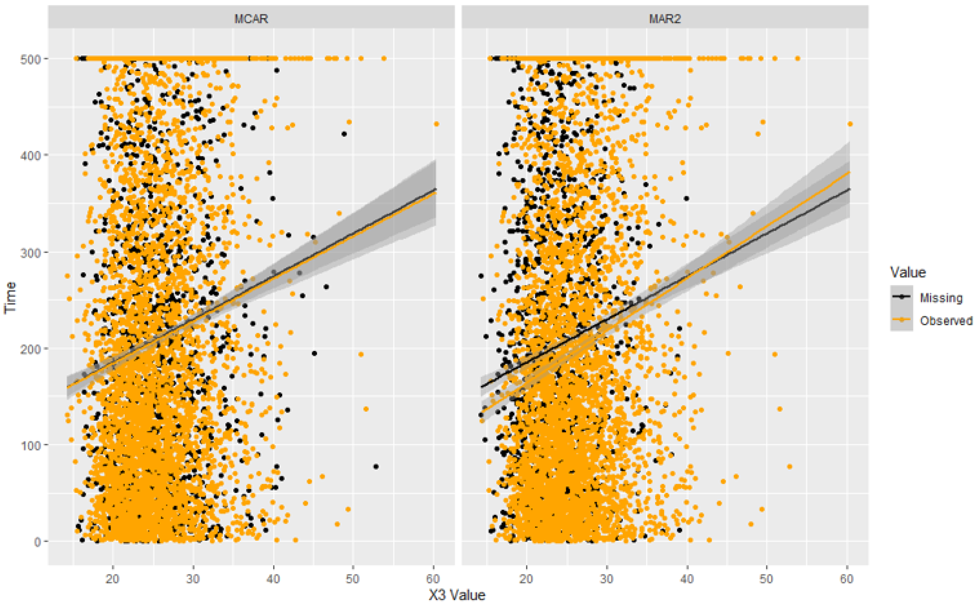
This in turn affects the relationship between X 3 and the outcome variable as shown in Figure 2. While this relationship is preserved under MCAR missingness, there are clear differences in the relationship between ‘survival time’ and, respectively, the observed and the missing values of X 3 under MAR2. Imputing the missing values from the distribution of the observed values may thus result in estimated coefficients further from the true value of β 3 and thus increased PB and undercoverage.

4. Discussion

In this paper we have undertaken a simulation study within a survival analysis context to investigate various aspects of MI. Whilst the study is modest in scale and in no way definitive, a number of aspects are worthy of attention.
First, it is rare to know for sure what the missingness mechanism is in a real application and clearly just because an imputation method performs well under an MCAR structure, it need not do so under a MAR structure. In practice it may be that a chosen MI approach with good MCAR properties may perform less well if the missingness (unbeknown to the analyst) is MAR. So, anything that can help the performance of such an MI method is to be welcomed. In our study, at least under the MAR1 structure, the presence of an auxiliary variable can be useful. For example, FCS-PMM-APA with no auxiliary variable has a low CR but its CR is reasonable in this case when an auxiliary variable is present. Conversely, in our study if an MI method performs well with no auxiliary variable (for example, SMCFCS-BLR-LNP under MAR2), it retains a good performance in the presence of an auxiliary variable. So, the indication is that if an appropriate auxiliary variable is available, it is worth considering incorporating it into the MI approach.
Secondly, we are interested in this study, in simple terms, about whether active or passive MI is preferable in a survival analysis context with BMI. In our study active imputation methods have performed well (FCS-BLR-APA) and poorly (FCS-PMM-AWO). Likewise passive imputation methods have performed well (FCS-BLR-PNP) and poorly (FCS-PMM-PNP). So the general question “which is better, active or passive imputation?” is too simplistic. Rather, it is important also to bring in other factors, such as whether to use BLR or PMM in further studies or in practice.
Thirdly, the idea of logging a ratio before undertaking imputation seems like an obvious thing to do. Typically, ratios like BMI are positive and positively skewed. Basic statistics indicates that taking logs of such variables may make them less skewed. But in our study pre-imputation logging is not always beneficial; for example, FCS-PMM-LNP did not perform well with MAR2 and no auxiliary variable. On the other hand, SMCFCS-BLR-LNP was arguably the best performing approach in our study. So, it is important to bring in other factors, such as whether to use FCS or SMCFCS in further studies or in practice.
Fourthly, Ref. [3] noted that more investigation of SMCFCS in a censored data context is needed. We concur with this given the results in the present study where SMCFCS-BLR-LNP in particular performed well in all scenarios. In addition, for BLR-PNP, SMCFCS showed improved performance compared with FCS.
The main limitation of our study is the focus on the exponential model as the substantive model, combined with a Type I censoring scheme albeit for different sample sizes and censoring percentages. While we have found several interesting results for these scenarios with different missingness mechanisms and in the presence/absence of an auxiliary variable, it would be interesting to see if our conclusions generalise to further widely used survival models, such as the Weibull model or Cox’s proportional hazards model, with a variety of commonly encountered censoring schemes. Further avenues of interest that could be explored in future research include investigating different composite covariates and different percentages of missingness in the composite covariate and its constituents. Realistic simulation scenarios could be based on survival studies beyond those on organ transplantation, to broaden the appeal, and to increase the benefits, to practitioners in the area of survival studies.

Supplementary Materials

The following supporting information can be downloaded at: https://www.mdpi.com/article/10.3390/stats5020020/s1, Tables S1–S3: PB, CR, and AW for the estimated coefficients of the composite covariate in a exponential AFT substantive model when N = 500 at 10%, 15% and 20% of observations are censored; Tables S4–S6: PB, CR, and AW for the estimated coefficients of the composite covariate in a exponential AFT substantive model when N = 1000 at 10%, 15% and 20% of observations are censored; Tables S7 and S8: PB, CR, and AW for the estimated coefficients of the composite covariate in a exponential AFT substantive model when N = 2000 at 10% and 20% of observations are censored.

Author Contributions

Conceptualization, L.C., A.C.K. and S.B.; methodology, L.C., A.C.K. and S.B.; software, L.C.; validation, L.C., A.C.K. and S.B.; formal analysis, L.C.; investigation, L.C.; writing—original draft preparation, L.C.; writing—review and editing, A.C.K. and S.B.; supervision, A.C.K. and S.B. All authors have read and agreed to the published version of the manuscript.

Funding

Lily Clements’s research was funded by an EPSRC PhD studentship at the University of Southampton.

Data Availability Statement

Data generated in the simulation study can be found at https://github.com/lilyclements/mice-data (accessed on 1 February 2022). The kidney transplant data we used to motivate our simulation scenarios can be found at https://www.odt.nhs.uk/statistics-and-reports/access-data/ (accessed on 1 February 2022) and the National Health and Nutrition Examination Survey can be found at https://wwwn.cdc.gov/nchs/nhanes/continuousnhanes/default.aspx?BeginYear=1999 (accessed on 1 February 2022).

Conflicts of Interest

The authors declare no conflict of interest.

Abbreviations

The following abbreviations are used in this manuscript:
BMIBody Mass Index
MIMultiple Imputation
FCSFully Conditional Specification
SMCFCSSubstantive Model Compatible Fully Conditional Specification
MCARMissing Completely at Random
MARMissing at Random
BLRBayesian Linear Regression
PMMPredictive Mean Matching
MAR1First MAR structure used in the simulation study
MAR2Stricter MAR structure used in the simulation study
AWOActive Imputation when the constituents are not predictors
APAActive Imputation when the constituents are predictors
PNPStandard Passive Imputation
LNPPassive Imputation when the constituents are first log-transformed
PBPercentage Bias
CRCoverage Rate
AWAverage Width
FMIFraction of Missing Information
RIVRelative Increase of Variance

References

  1. Rubin, D.B. Multiple imputations in sample surveys—A phenomenological Bayesian approach to nonresponse. In Proceedings of the Survey Research Methods Section of the American Statistical Association, Alexandria, VA, USA, 2 January 1978; Volume 1, pp. 20–34. [Google Scholar]
  2. Pankhurst, L.; Mitra, R.; Kimber, A.C.; Collett, D. Multiply imputing missing values arising by design in transplant survival data. Biom. J. 2020, 62, 1192–1207. [Google Scholar] [CrossRef] [PubMed] [Green Version]
  3. Bartlett, J.W.; Morris, T.P. Multiple imputation of covariates by substantive-model compatible fully conditional specification. Stata J. 2015, 15, 437–456. [Google Scholar] [CrossRef] [Green Version]
  4. Carpenter, J.; Kenward, M. Multiple Imputation and Its Applications; Wiley and Sons: Hoboken, NJ, USA, 2012. [Google Scholar]
  5. Rubin, D.B. Inference and missing data. Biometrika 1976, 63, 581–592. [Google Scholar] [CrossRef]
  6. Rubin, D.B. Multiple Imputation for Survey Nonresponse; John Wiley & Sons: Hoboken, NJ, USA, 1987. [Google Scholar]
  7. Azur, M.J.; Stuart, E.A.; Frangakis, C.; Leaf, P.J. Multiple imputation by chained equations: What is it and how does it work? Int. J. Methods Psychiatr. Res. 2011, 20, 40–49. [Google Scholar] [CrossRef]
  8. van Buuren, S. Flexible Imputation of Missing Data; Chapman and Hall/CRC: Boca Raton, FL, USA, 2018. [Google Scholar]
  9. White, I.R.; Royston, P.; Wood, A.M. Multiple imputation using chained equations: Issues and guidance for practice. Stat. Med. 2011, 30, 377–399. [Google Scholar] [CrossRef] [PubMed]
  10. Burton, A.; Altman, D.G.; Royston, P.; Holder, R.L. The design of simulation studies in medical statistics. Stat. Med. 2006, 25, 4279–4292. [Google Scholar] [CrossRef] [PubMed]
  11. van Buuren, S. Package ‘Mice’. Available online: https://github.com/cran/mice (accessed on 1 January 2022).
  12. Bartlett, J.; Keogh, R.; Bonneville, E.; Ekstrøm, C. Package ‘Smcfcs’. Available online: https://github.com/jwb133/smcfcs (accessed on 1 February 2021).
  13. Wagstaff, D.A.; Kranz, S.; Harel, O. A preliminary study of active compared with passive imputation of missing body mass index values among non-Hispanic white youths. Am. J. Clin. Nutr. 2009, 89, 1025–1030. [Google Scholar] [CrossRef] [PubMed]
  14. Morris, T.P.; White, I.R.; Royston, P.; Seaman, S.R.; Wood, A.M. Multiple imputation for an incomplete covariate that is a ratio. Stat. Med. 2014, 33, 88–104. [Google Scholar] [CrossRef] [Green Version]
  15. von Hippel, P.T. How to impute interactions, squares, and other transformed variables. Sociol. Methodol. 2009, 39, 265–291. [Google Scholar] [CrossRef]
  16. van Buuren, S. MICE: Passive Imputation and Post-Processing. Available online: https://www.gerkovink.com/miceVignettes/Passive_Post_processing/Passive_imputation_post_processing.html (accessed on 11 March 2019).
  17. Enders, C.K. Applied Missing Data Analysis; Guilford Press: New York, NY, USA, 2010. [Google Scholar]
  18. Eddings, W. A Note on How to Perform Multiple-Imputation Diagnostics in Stata. Available online: http://www.stata.com/users/ymarchenko/midiagnote.pdf (accessed on 20 May 2020).
  19. Brown, L.D.; Cai, T.T.; DasGupta, A. Interval estimation for a binomial proportion. Stat. Sci. 2001, 16, 101–133. [Google Scholar] [CrossRef]
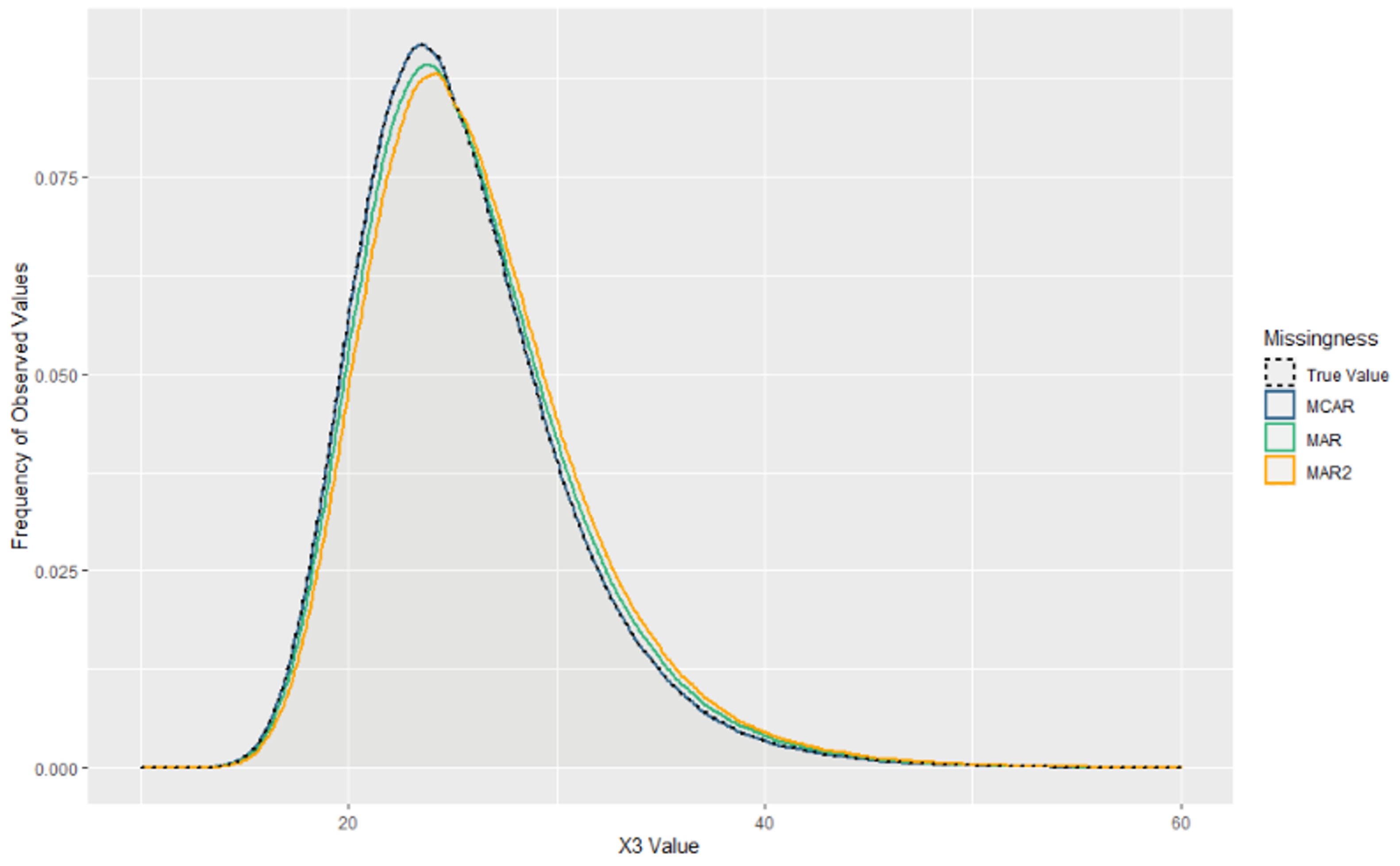
Figure 1. Kernel density plot of observed X 3 values for the different missingness structures, and for X 3 when no missing values are generated.
Stats 05 00020 g001
Figure 2. The relationship between X 3 and survival time, split by whether X 3 is missing or observed. These plots are displayed for an MCAR missingness structure and an MAR2 missingness structure. The values plotted are a random sample of three generated data sets of 2000 values each.
Stats 05 00020 g002
Table 1. PB, CR, and AW for the estimated coefficients of the composite covariate in a exponential AFT substantive model when N = 2000 and 15% of observations are censored.
No Auxiliary VariablesOne Auxiliary Variable
PBCR (%)AWPBCR (%)AW
MCARFCS-BLRAWO1.4495.10.02390.8896.20.0231
APA1.2896.30.02300.8896.60.0224
PNP3.1295.10.02282.7695.50.0223
LNP0.2695.70.02310.0896.70.0226
FCS-PMMAWO1.9294.30.02381.8295.90.0229
APA1.1496.00.02320.5896.70.0222
PNP0.8695.60.02320.2496.80.0221
LNP0.6095.80.02310.1696.80.0224
SMCFCS-BLRPNP0.0696.50.02280.0296.20.0222
LNP0.5496.40.02300.9896.50.0224
MAR1FCS-BLRAWO1.6695.10.02310.2895.80.0224
APA0.9696.20.02230.2096.10.0219
PNP1.0896.70.02221.8495.60.0217
LNP2.5695.30.02241.7496.00.0221
FCS-PMMAWO2.4695.00.02321.5496.20.0222
APA4.8093.10.02262.9695.10.0217
PNP4.4693.40.02262.4695.90.0216
LNP2.9095.30.02251.9496.10.0219
SMCFCS-BLRPNP0.1296.80.02211.0696.10.0216
LNP0.5896.20.02230.3496.00.0218
MAR2FCS-BLRAWO4.4693.30.02241.3294.80.0219
APA2.5695.10.02180.7694.80.0215
PNP0.3295.20.02171.3494.50.0213
LNP4.6492.40.02202.8494.60.0217
FCS-PMMAWO0.6476.70.02313.2093.70.0216
APA7.1288.40.02234.4093.30.0213
PNP6.8888.80.02223.8892.90.0212
LNP5.2491.20.02213.2693.80.0216
SMCFCS-BLRPNP0.7494.50.02122.4494.20.0210
LNP0.1095.40.02180.8095.10.0214
Table 2. Mean FMI and mean RIV values for β ^ 3 over the 1000 replications for all imputation models.
No Auxiliary VariablesOne Auxiliary Variable
FMIRIVFMIRIV
MCARFCS-BLRAWO0.3040.4360.2560.344
APA0.2440.3220.2090.263
PNP0.2590.3480.2230.286
LNP0.2240.2880.1930.238
FCS-PMMAWO0.2810.3900.2450.324
APA0.2290.2960.1970.244
PNP0.2300.2970.2000.249
LNP0.2250.2890.1950.241
SMCFCS-BLRPNP0.2420.3260.2040.260
LNP0.2160.2800.1790.222
MAR1FCS-BLRAWO0.2960.4200.2500.333
APA0.2310.3000.2040.255
PNP0.2490.3310.2180.278
LNP0.2020.2520.1750.211
FCS-PMMAWO0.2470.3280.2100.264
APA0.2080.2620.1790.217
PNP0.2070.2600.1800.218
LNP0.1990.2480.1740.210
SMCFCS-BLRPNP0.2320.3090.1970.249
LNP0.1910.2400.1580.190
MAR2FCS-BLRAWO0.2860.4000.2430.320
APA0.2230.2860.1960.243
PNP0.2400.3140.2100.265
LNP0.1850.2260.1590.188
FCS-PMMAWO0.2480.3440.1780.215
APA0.1880.2310.1610.191
PNP0.1880.2300.1610.191
LNP0.1780.2150.1540.181
SMCFCS-BLRPNP0.2220.2890.1890.236
LNP0.1690.2060.1390.163
Publisher’s Note: MDPI stays neutral with regard to jurisdictional claims in published maps and institutional affiliations.