Bayesian Semiparametric Regression Analysis of Multivariate Panel Count Data

Abstract

Panel count data often occur in a long-term recurrent event study, where the exact occurrence time of the recurrent events is unknown, but only the occurrence count between any two adjacent observation time points is recorded. Most traditional methods only handle panel count data for a single type of event. In this paper, we propose a Bayesian semiparameteric approach to analyze panel count data for multiple types of events. For each type of recurrent event, the proportional mean model is adopted to model the mean count of the event, where its baseline mean function is approximated by monotone I-splines. The correlation between multiple types of events is modeled by common frailty terms and scale parameters. Unlike many frequentist estimating equation methods, our approach is based on the observed likelihood and makes no assumption on the relationship between the recurrent process and the observation process. Under the Poisson counting process assumption, we develop an efficient Gibbs sampler based on novel data augmentation for the Markov chain Monte Carlo sampling. Simulation studies show good estimation performance of the baseline mean functions and the regression coefficients; meanwhile, the importance of including the scale parameter to flexibly accommodate the correlation between events is also demonstrated. Finally, a skin cancer data example is fully analyzed to illustrate the proposed methods.

1. Introduction

Panel count data often arise in epidemiological and medical studies, in which the events of interest have a property of recurring and subjects are monitored periodically. Since the subjects are not under continuous monitoring, the exact time of each recurrent event is not observed but the count of such events between adjacent observation times is known. Many times in a study, several types of related recurrent events are of interest to be collected. For example, the recurrent events can be different types of infections, tumors, and social behaviors such as drinking and drug use. The motivating example is bivariate panel count data on skin cancers from the literature [1]. The data arose from a skin cancer chemoprevention trial conducted by the University of Wisconsin Comprehensive Cancer Center. This was a double-blinded and placebo-controlled randomized III clinical trial. The main objective of the study was to evaluate the effectiveness of 0.5/m${}^2$/day PO difluoromethylornithine (DFMO) in reducing the recurrence rate of skin cancers in a population of patients with a history of non-melanoma skin cancers: basal cell carcinoma and squamous cell carcinoma. Two hundred and ninety one patients were randomized into either a placebo group or a DFMO group. During the study, the patients were scheduled to regularly take 6-month reviews to check the development of both skin cancers. At each visit, the numbers of occurrences of both basal cell carcinoma and squamous cell carcinoma since the previous visit were recorded. For these bivariate panel count data, it is possible to analyze these two skin cancers separately to evaluate the effectiveness of DFMO. However, conducting a joint analysis is a better practice to investigate the correlation between two cancers and to improve the estimation efficiency.

Extensive methods have been established to analyze panel count data for a single type of recurrent event, for example Sun and Kalbfleisch [2], Sun and Zhao [1], Wellner and Zhang [3,4], Lu et al. [5,6], Wang and Lin [7], among others. For multivariate panel count data, He et al. [8] considered regression analysis for multivariate panel count data and first proposed a class of marginal mean models, which leave the dependence structures for related recurrent events completely unspecified. Zhang et al. [9] then improved their model and provided a robust joint modeling approach for the regression analysis of multivariate panel count data with an informative observation process. Li et al. [10] proposed semiparametric transformation models that allow the dependence of the recurrent event processes on the observation process. Along the same line, Zhao et al. [11] proposed a semiparametric additive model to analyze the multivariate panel count data with dependent observation processes and a terminal event. This branch of works emphasize the dependence of the recurrent event processes on the observation process and require the model of the observation process being explicitly specified. They usually derive estimating equation methods to estimate regression coefficient without estimating baseline mean functions.

Another line of research for panel count data is to consider varying or nonlinear covariate effects. He et al. [12] proposed a class of partially linear models with varying coefficients for the mean function of the counting processes to explore the nonlinear interactions between covariates. Zhao et al. [13] adopted the B-splines to model the regression function. Wang and Yu [14] proposed the time varying coefficient model by the local linear expansion method. For multivariate panel count data, Li et al. [15] presented a joint modeling for the recurrent event processes, observation process, and censoring time by using time-dependent random effects. Wang and Yu [16] proposed a varying coefficient mean model for multivariate panel count data to describe the possible nonlinear interact effects between covariates. In this paper, instead of investigating varying covariate effects, we only focus on traditional constant covariate effects.

Frequentist approaches dominate the analysis of panel count data. There is only a limited number of papers describing Bayesian approaches for analyzing panel count data. Chib et al. [17] investigated estimation and model comparison for panel count data models with multiple random effects. Sinha and Maiti (2004) proposed a Bayesian approach for the analysis of panel count data with dependent termination. Wang and Lin (2020) developed a Bayesian semiparametric approach under the proportional mean model with the baseline mean function approximated by monotone I-splines [18]. Dimitrakopoulos [19] discussed how Bayesian techniques can be used to estimate the panel count data model. Liang et al. [20] proposed a bivariate Gaussian Cox process model to jointly model the recurrent event process and the observation process. To the best of our knowledge, Ref. [20] is the only Bayesian paper for analyzing multivariate panel count data.

In this paper, we contribute a new Bayesian semiparameteric approach to analyze panel count data for multiple types of recurrent events. For each type of recurrent event, we adopt the modeling in Wang and Lin (2020) by using the proportional mean model to model the mean count of the recurrent event with its baseline mean function approximated by monotone I-splines [18]. The proposed approach is based on the observed likelihood using only the observed counts and observation times, which does not require us to specify a model for the observation process. Instead of building up the correlation among multiple types of events through their dependence on the observation process, we tackle the correlations between different types of events directly by introducing common subject-specific gamma frailty terms and additional scale parameters. The resulting pairwise correlations can be calculated in a close form and flexibly accommodate different correlation situations including positive, negative, strong, and weak correlations. Based on Poisson latent variable augmentation, our developed MCMC algorithm can estimate both the regression coefficients and the baseline mean functions simultaneously.

The remainder of this paper is organized as follows. In Section 2, primary models and the correlation derivation and interpretation are introduced. In Section 3, a detailed description of monotone I-splines, augmented likelihood function construction, and prior specification and posterior computation are presented. Section 4 evaluates our proposed methods via extensive simulation studies. The skin cancer data are used to demonstrate the performance of the proposed methods in Section 5. Lastly, Section 6 summarizes our findings and discusses some future work directions.

2. Model and Notation

2.1. Model Construction

Consider that n subjects participate a long-term study involving K types of related recurrent events. Each subject is not under continuous monitoring and instead observed at discrete time points. Specifically, for each subject i, $J_i^{\left(k\right)}$ denotes the total number of observation times for event k, and the corresponding observation times are $0=t_{i0}^{\left(k\right)}<t_{i1}^{\left(k\right)}<t_{i2}^{\left(k\right)}<\dots <t_{i{J}_i^{\left(k\right)}}^{\left(k\right)}$. Let $N_i^{\left(k\right)}\left(t\right)$ denote the cumulative count of the occurrence of event k prior to time t for subject i. Let $X_i^{\left(k\right)}={(x_{i1}^{\left(k\right)},\dots ,x_{ip}^{\left(k\right)})}^{\prime }$ denote the $p\times 1$ covariate vector associated with subject i for event k. For simplicity, in this paper we assume the covariates for subject i are identical for all K events and denoted by $X_i$. The whole set of observed panel count data is denoted by $\mathcal{D}$$=\{t_{ij}^{\left(k\right)},N_i^{\left(k\right)}\left(t_{ij}^{\left(k\right)}\right),X_i,fork=1,\dots ,K;i=1,\dots ,n;j=1,\dots ,J_i^{\left(k\right)}\}$. Finally, we assume there is a latent subject-specific positive frailty term $w_i$ for each subject i, which affects the occurrence rates and connects the multiple events. The frailties $w_i$’s are assumed to follow a gamma distribution $\mathcal{G}(\eta ,\eta )$ with mean 1 and variance $1/\eta$. The model identifiability is satisfied with the mean of frailties equal to 1 [21,22]. Given the covariates $X_i$ and frailty $w_i$, we assume the counting process {$N_i^{\left(k\right)}\left(t\right),t>0$} for event k has a proportional mean function in the following form:

$$E\left(N_i^{\left(k\right)}\left(t\right)|X_i,w_i\right)=w_i^{{\alpha }_k}{U}_0^{\left(k\right)}\left(t\right)exp\left(X_i^{\prime }{\mathbf{\beta }}^{\left(k\right)}\right),$$

(1)

where ${\alpha }_k$ is a scale parameter introduced to more flexibly accommodate the correlation between events, $U_0^{\left(k\right)}\left(t\right)$ is the baseline mean function for event k, and ${\mathbf{\beta }}^{\left(k\right)}$ is a $p\times 1$ vector of regression coefficients for event k. By default, the model considers different covariate effects for different recurrent events, but it is easy to extend to the situation where the covariate effects are identical across all the K events. More details about ${\alpha }_k$ related to the correlation are discussed in Section 2.2.

Let $Z_{ij}^{\left(k\right)}$ denote the number of occurrence of event k in the jth time interval $(t_{i,j-1}^{\left(k\right)},t_{ij}^{\left(k\right)}]$ for subject i, i.e., $Z_{ij}^{\left(k\right)}=N_i^{\left(k\right)}\left(t_{ij}^{\left(k\right)}\right)-N_i^{\left(k\right)}\left(t_{i,j-1}^{\left(k\right)}\right)$, where we assume $N_i^{\left(k\right)}\left(t_{i0}\right)=0$ for $i=1,\dots ,n.$ Through this transformation, the whole set of data can be expressed as $\mathcal{D}$$=\{t_{ij}^{\left(k\right)},Z_{ij}^{\left(k\right)},X_i,fork=1,\dots ,K;i=1,\dots ,n;j=1,\dots ,J_i^{\left(k\right)}\}$. Under the Poisson process assumption, given the covariates $X_i$ and latent frailty terms $w_i$, $Z_{ij}^{\left(k\right)}$ independently follows Poisson distributions, which can be written as:

$$Z_{ij}^{\left(k\right)}|X_i,w_i\sim \mathcal{P}\left(w_i^{{\alpha }_k}\{U_0^{\left(k\right)}\left(t_{ij}^{\left(k\right)}\right)-U_0^{\left(k\right)}\left(t_{i,j-1}^{\left(k\right)}\right)\}exp\left(X_i^{\prime }{\mathbf{\beta }}^{\left(k\right)}\right)\right).$$

(2)

This form is particularly useful for constructing the likelihood function in Section 3.2. Note that when integrating out the frailty effect $w_i$, $Z_{ij}^{\left(k\right)}$ marginally follows mixed Poisson distributions [1].

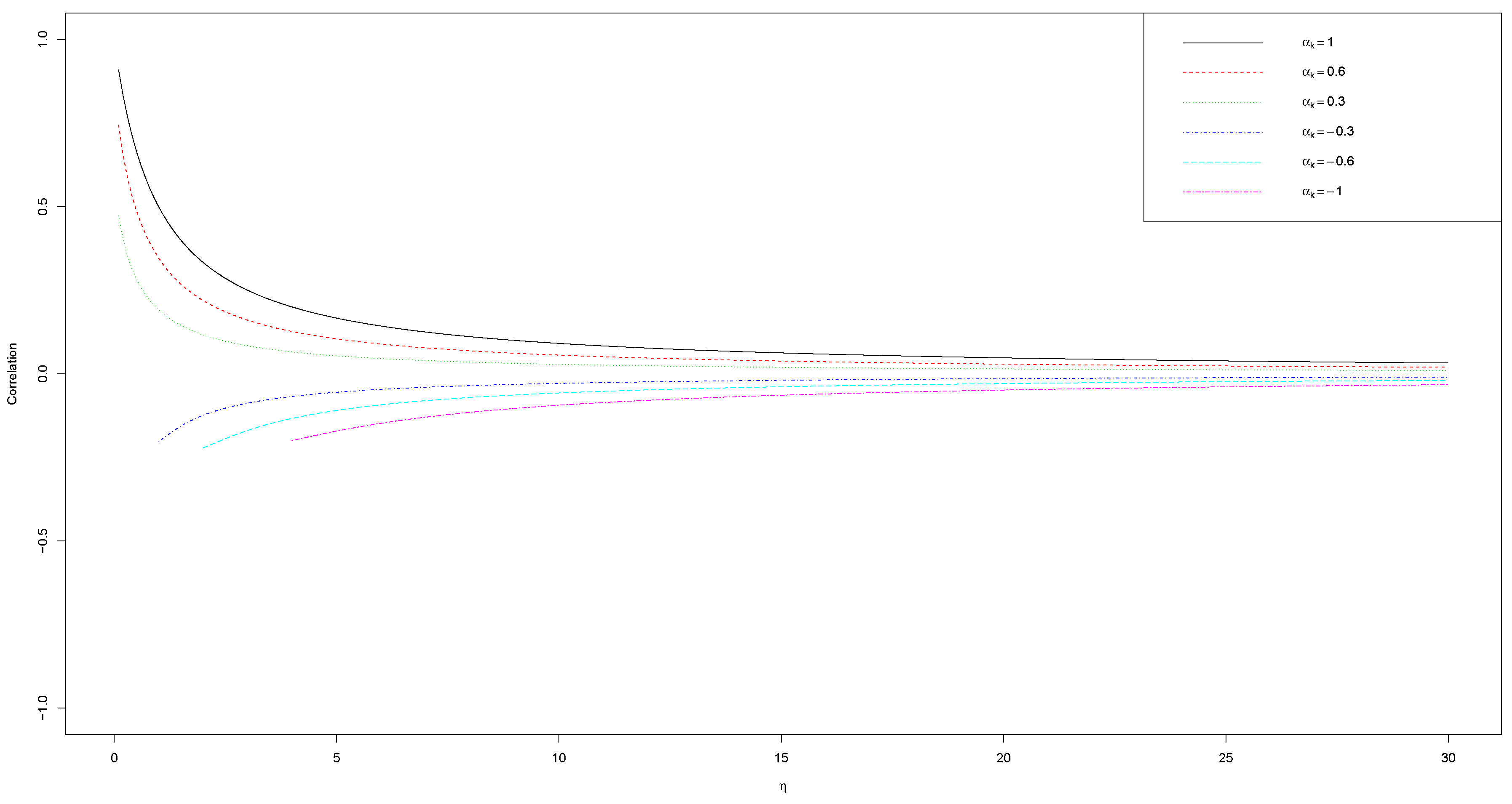
2.2. Correlation Expression

An advantage of our proposed model is its straightforwardness in deriving the correlation formula between two events. Among the K events, we predesignate one event that is of main interest, for instance event j, as a reference event, and let ${\alpha }_j=1$. Then, given the covariates $X_i$ and the unobservable frailty $w_i$, the cumulative counts of event j and event k ($k\ne j$) for subject i at any time point t are conditionally independent and have

$$N_i^{\left(j\right)}\left(t\right)|X_i,w_i\sim \mathcal{P}\left(w_i{U}_0^{\left(j\right)}\left(t\right)exp\left(X_i^{\prime }{\mathbf{\beta }}^{\left(j\right)}\right)\right),$$

$$N_i^{\left(k\right)}\left(t\right)|X_i,w_i\sim \mathcal{P}\left(w_i^{{\alpha }_k}{U}_0^{\left(k\right)}\left(t\right)exp\left(X_i^{\prime }{\mathbf{\beta }}^{\left(k\right)}\right)\right).$$

Using the law of total variance, we explicitly derive $Cov\left(N_i^{\left(j\right)}\left(t\right),N_i^{\left(k\right)}\left(t\right)\right)$, $Var\left(N_i^{\left(j\right)}\left(t\right)\right)$ and $Var\left(N_i^{\left(k\right)}\left(t\right)\right)$ and hence the correlation formula as below:

$$\begin{array}{cc}\hfill Corr\left(N_i^{\left(j\right)}\left(t\right),N_i^{\left(k\right)}\left(t\right)\right)& =\frac{Cov\left(N_i^{\left(j\right)}\left(t\right),N_i^{\left(k\right)}\left(t\right)\right)}{\sqrt{Var\left(N_i^{\left(j\right)}\left(t\right)\right)Var\left(N_i^{\left(k\right)}\left(t\right)\right)}}\hfill \\ \hfill & =\frac{{\alpha }_k}{\sqrt{\eta +\frac{{\eta }^2}{[U_0^{\left(j\right)}\left(t\right)exp\left(X_i^{\prime }{\mathbf{\beta }}^{\left(j\right)}\right)]}}\sqrt{\frac{\Gamma (\eta +2{\alpha }_k)\Gamma \left(\eta \right)}{{(\Gamma (\eta +{\alpha }_k))}^2}-1+\frac{\Gamma \left(\eta \right){\eta }^{{\alpha }_k}}{\Gamma (\eta +{\alpha }_k)[U_0^{\left(k\right)}\left(t\right)exp\left(X_i^{\prime }{\mathbf{\beta }}^{\left(k\right)}\right)]}}}\hfill \end{array}$$

(3)

where $\eta >0$ and ${\alpha }_k>-\eta /2$. For details on derivation of Equation (3), see Appendix A. Clearly, ${\alpha }_k=0$ implies that event j and event k are independent; ${\alpha }_k>0$ implies that event j and event k are positively related; ${\alpha }_k<0$ implies that event j and event k are negatively related. When getting rid of the covariate effects, the baseline correlation between the two events is

$$Cor{r}_0\left(N^{\left(j\right)}\left(t\right),N^{\left(k\right)}\left(t\right)\right)=\frac{{\alpha }_k}{\sqrt{\eta +\frac{{\eta }^2}{U_0^{\left(j\right)}\left(t\right)}}\sqrt{\frac{\Gamma (\eta +2{\alpha }_k)\Gamma \left(\eta \right)}{{(\Gamma (\eta +{\alpha }_k))}^2}-1+\frac{\Gamma \left(\eta \right){\eta }^{{\alpha }_k}}{\Gamma (\eta +{\alpha }_k)U_0^{\left(k\right)}\left(t\right)}}}.$$

The benefit of this form is that it gets away with the individual level and provides a broader view of the correlation between two events. Letting $U_0^{\left(j\right)}\left(t\right)=U_0^{\left(k\right)}\left(t\right)=1$, we can explore the pure effect of ${\alpha }_k$ and $\eta$ on the baseline correlation $Cor{r}_0(N^{\left(j\right)}\left(t\right),N^{\left(k\right)}\left(t\right))$. Note that the correlation between any two events is controlled by the parameters $\eta$ and ${\alpha }_k$. Figure A1 shows the baseline correlation performance related to $\eta$ and ${\alpha }_k$ when ${\alpha }_k\in [-1,1]$. It shows that with the variance of frailty increasing ($\eta$ decreasing), the correlation increases; with the magnitude of ${\alpha }_k$ increasing, the correlation also increases. When ${\alpha }_k>0$, any $\eta >0$ is a legitimate choice; while for ${\alpha }_k<0$, the condition $\eta >-2{\alpha }_k$ must be satisfied to make $\Gamma (·)$ valid. In fact, the interpretation of the pairwise correlation is not limited to the pairs of events involving the predesignated event. A similar derivation can derive the correlation between any two types of events. Theoretically, ${\alpha }_k$ can be any value greater than $-\eta /2$. We only choose ${\alpha }_k$ between −1 and 1 because we think in practice we can always choose the event with the largest frailty variability as the reference event. Then, for the other events, we only need ${\alpha }_k$ between $-1$ and 1.

3. The Proposed Bayesian Semiparametric Approach

3.1. Modeling $U_0^{\left(k\right)}\left(t\right)$ with Monotone I-Splines

To accommodate the nondecreasing nature of the baseline mean functions in the proposed model, we choose monotone I-splines to model them. I-splines were first bought up by Ramsay [18] and then widely applied in many semiparametric models. To put it briefly, I-splines are actually integrated M-splines, a set of non-negative spline functions [18]. In our proposed model, each baseline function of event k is modeled as a linear combination of I-splines:

$$U_0^{\left(k\right)}\left(t\right)=\sum _{l=1}^L{r}_l^{\left(k\right)}{I}_l\left(t\right|d),$$

(4)

In the formula, $I_l(·|d)$ is the I-spline basis function with degree d; L is the number of I-spline basis functions, which equals the number of interior knots plus the degree d; $r_l^{\left(k\right)}$s are the nonnegative spline coefficients. For more detailed information on the formula of I-splines, refer to Ramsay [18] and Lin et al. [23]. The degree d and the placement of knots are two chief components that determine the basis functions. The former controls the smoothness and the latter controls the shape of the spline function. In general, 2 or 3 degrees is enough to provide adequate smoothness, and 10 to 30 knots can provide enough flexibility for a regression incorporating thousands of observations according to Cai et al. [24] and Wang and Dunson [25]. Equally spaced knots and quantile-based knots are two commonly used methods to select knots. Ref. [7] showed that the deviance information criterion (DIC) can be used to facilitate choosing the setup for the I-spline functions. In addition, reversible jump MCMC technique [26] may also help adaptively choosing the number and location of knots. In this paper, to avoid additional computation burden, we uniformly use degree 3 and 20 equally spaced knots (18 interior knots), which provides sufficient flexibility for modeling the unknown baseline mean functions.

3.2. Likelihood Augmentation with Poisson Latent Variables

Consider that n subjects participate in a long-term study involving K types of related recurrent events. The data structure and model are defined in Section 2.1. Under the Poisson process assumption, following Equation (2), the observed likelihood function can be written in the following form:

$$L_{obs}=\prod _{k=1}^K\prod _{i=1}^n\prod _{j=1}^{J_i^{\left(k\right)}}exp[-w_i^{{\alpha }_k}\{U_0^{\left(k\right)}\left(t_{i,j}^{\left(k\right)}\right)-U_0^{\left(k\right)}\left(t_{i,j-1}^{\left(k\right)}\right)\}exp\left(X_i^{\prime }{\mathbf{\beta }}^{\left(k\right)}\right)]$$

$$\times [w_i^{{\alpha }_k}\{U_0^{\left(k\right)}\left(t_{ij}^{\left(k\right)}\right)-U_0^{\left(k\right)}\left(t_{i,j-1}^{\left(k\right)}\right)\}exp\left(X_i^{\prime }{\mathbf{\beta }}^{\left(k\right)}\right){]}^{Z_{ij}^{\left(k\right)}}/Z_{ij}^{\left(k\right)}!$$

Taking the baseline function $U_0^{\left(k\right)}\left(t\right)$ in the form of (4), the likelihood can further be written as

$$L\left(\mathbf{\theta }\right|\mathcal{D})=\prod _{k=1}^K\prod _{i=1}^n\prod _{j=1}^{J{i}^{\left(k\right)}}exp[-w_i^{{\alpha }_k}\sum _{l=1}^L{r}_l^{\left(k\right)}\{I_l\left(t_{i,j}^{\left(k\right)}\right)-I_l\left(t_{i,j-1}^{\left(k\right)}\right)\}exp\left(X_i^{\prime }{\mathbf{\beta }}^{\left(k\right)}\right)]$$

$$\times [w_i^{{\alpha }_k}\sum _{l=1}^L{r}_l^{\left(k\right)}\{I_l\left(t_{i,j}^{\left(k\right)}\right)-I_l\left(t_{i,j-1}^{\left(k\right)}\right)\}exp\left(X_i^{\prime }{\mathbf{\beta }}^{\left(k\right)}\right){]}^{Z_{ij}^{\left(k\right)}}/Z_{ij}^{\left(k\right)}!$$

where $\mathbf{\theta }$ represents the vector of all unknown parameters including ${\mathbf{\beta }}^{\left(k\right)}={({\beta }_1^{\left(k\right)},\dots ,{\beta }_p^{\left(k\right)})}^{\prime }$ and $r^{\left(k\right)}={(r_1^{\left(k\right)},\dots ,r_L^{\left(k\right)})}^{\prime }$$fork=1,\dots ,K$, and $\alpha ={({\alpha }_1,\dots ,{\alpha }_k)}^{\prime }$. Note that for the simplicity of notation, the d is omitted from the I-spline basis functions. With this likelihood format, the sampling for $r_l^{\left(k\right)}$ is especially difficult. To solve this problem, we further decompose $Z_{ij}^{\left(k\right)}$ as ${\sum }_{l=1}^L{Z}_{ijl}^{\left(k\right)}$, where the augmented Poisson latent variables $Z_{ijl}^{\left(k\right)}$s independently follow Poisson distributions as follows:

$$Z_{ijl}^{\left(k\right)}|X_i,w_i\sim \mathcal{P}\left(w_i^{{\alpha }_k}\left\{r_l^{\left(k\right)}[I_l\left(t_{i,j}^{\left(k\right)}\right)-I_l\left(t_{i,j-1}^{\left(k\right)}\right)]\right\}exp\left(X_i^{\prime }{\mathbf{\beta }}^{\left(k\right)}\right)\right).$$

The convolution property of Poisson distribution aids the transformation smoothly. Then, with the augmented Poisson latent variables, the likelihood function can be expressed as

$$L_{aug}\left(\mathbf{\theta }\right|\mathcal{D})=\prod _{k=1}^K\prod _{i=1}^n\prod _{j=1}^{J_i^{\left(k\right)}}\prod _{l=1}^{L}exp[-w_i^{{\alpha }_k}{r}_l^{\left(k\right)}\{I_l\left(t_{i,j}^{\left(k\right)}\right)-I_l\left(t_{i,j-1}^{\left(k\right)}\right)\}exp\left(X_i^{\prime }{\mathbf{\beta }}^{\left(k\right)}\right)]$$

$$\times [w_i^{{\alpha }_k}{r}_l^{\left(k\right)}\{I_l\left(t_{i,j}^{\left(k\right)}\right)-I_l\left(t_{i,j-1}^{\left(k\right)}\right)\}exp\left(X_i^{\prime }{\mathbf{\beta }}^{\left(k\right)}\right){]}^{Z_{ijl}^{\left(k\right)}}/Z_{ijl}^{\left(k\right)}!.$$

(5)

Based on this augmented likelihood Equation (5), we develop the Bayesian computation algorithm in Section 3.3.

3.3. Prior Specification and Posterior Computation

For Bayesian computation, we need to first specify prior distributions for unknown parameters. When we do not have much prior information about parameters, we usually assign vague priors for them. For ${\mathbf{\beta }}_m^{\left(k\right)}$, $m=1,\dots ,p$; $k=1,\dots ,K$, we assign $\mathcal{N}(0,{\sigma }^2)$ priors, where ${\sigma }^2$ takes a large value such as 100. For nonnegative $r_l^{\left(k\right)}$, $l=1,\dots ,L$; $k=1,\dots ,K$, we assign exponential priors with rate parameter ${\lambda }_k$, where ${\lambda }_k$ itself follows a gamma prior $\mathcal{G}(a_{\lambda },b_{\lambda })$. This prior specification is appealing from the computational perspective because it leads to conjugate forms for each of the conditional posterior distributions of $r_l^{\left(k\right)}$ and ${\lambda }_k$. Theoretically, such a prior specification is closely related to Bayesian Lasso [27] and is equivalent to the penalized likelihood approach with an L1 penalty on those spline coefficients, in which ${\lambda }_k$ serve as tuning parameters. Our simulation studies show that our approach is robust to the choice of hyperparameters, so we simply choose $a_{\lambda }=1$ and $b_{\lambda }=1$. We adopt Gibbs sampling algorithm for posterior computation. Basically, we derive the full conditional distribution of each parameter component-wisely from the joint distribution of the likelihood function in (5) and the specified prior distributions. If the full conditional distribution of a parameter has a closed form, the sampling is straightforward. When the closed form is intractable, an adaptive rejection sample (ARS) [28] is adopted if the full conditional posterior distribution preserves the log-concavity. Even if the log concavity is not satisfied, we can still use adaptive rejection metropolis sampling (ARMS) [29] to draw samples. Specifically, we use function arms() in the R package HI [30] to realize the ARMS. The full conditional distributions of the Gibbs sampler are summarized as below.

• Sample ($Z_{ij1}^{\left(k\right)}$, …, $Z_{ijL}^{\left(k\right)}$) from a multinomial distribution $\mathcal{M}(Z_{ij}^{\left(k\right)},\mathit{P}{\left(k\right)}_{ij})$, for $i=1,\dots ,n;$$j=1,\dots ,$$J_i^{\left(k\right)}$; $k=1,\dots ,K$, where ${\mathit{P}}_{ij}^{\left(k\right)}=(p_{ij1}^{\left(k\right)},\dots ,p_{ijL}^{\left(k\right)})$ with ${\sum }_{l=1}^L{p}_{ijl}^{\left(k\right)}=1$, and

  $$p_{ijL}^{\left(k\right)}=\frac{r_l^{\left(k\right)}\left\{I_l\left(t_{ij}^{\left(k\right)}\right)-I_l\left(t_{i,(j-1)}^{\left(k\right)}\right)\right\}}{{\sum }_{l=1}^L{r}_l^{\left(k\right)}\left\{I_l\left(t_{ij}^{\left(k\right)}\right)-I_l\left(t_{i,(j-1)}^{\left(k\right)}\right)\right\}}.$$
• Sample $r_l^{\left(k\right)}$ from a Gamma distribution $\mathcal{G}(A_l^{\left(k\right)},B_l^{\left(k\right)})$, for $l=1,\dots ,L;k=1,\dots ,K$, with

  $$A_l^{\left(k\right)}=\sum _{i=1}^n\sum _{j=1}^{J_i^{\left(k\right)}}{Z}_{ijl}^{\left(k\right)}+1,$$

  and

  $$B_l^{\left(k\right)}=\sum _{i=1}^n{w}_i^{{\alpha }_k}\left\{I_l\left(t_{i{J}_i^{\left(k\right)}}^{\left(k\right)}\right)-I_l\left(t_{i0}^{\left(k\right)}\right)\right\}exp\left(X_i^{\prime }{\mathbf{\beta }}^{\left(k\right)}\right)+{\lambda }_k.$$
• Sample ${\lambda }_k$ from a Gamma distribution $\mathcal{G}(a_{\lambda }+L,b_{\lambda }+{\sum }_{l=1}^L{r}_l^{\left(k\right)})$, for $k=1,\dots ,K$.
• Sample ${\beta }_m^{\left(k\right)}$ by using the adaptive rejection sampling (ARS) [28] method, for $m=1,$$\dots ,p;k=1,\dots ,K$. The log full conditional distribution of each ${\beta }_m$ is proportional to

  $$exp[-\sum _{i=1}^n\sum _{l=1}^L{w}_i^{{\alpha }_k}{r}_l^{\left(k\right)}\left\{I_l\left(t_{i{J}_i^{\left(k\right)}}^{\left(k\right)}\right)-I_l\left(t_{i0}^{\left(k\right)}\right)\right\}exp\left(X_i^{\prime }{\mathbf{\beta }}^{\left(k\right)}\right)+\sum _{i=1}^n\sum _{j=1}^{J_i^{\left(k\right)}}{X}_i^{\prime }{\mathbf{\beta }}^{\left(k\right)}{Z}_{ij}^{\left(k\right)}-{\left({\beta }_m^{\left(k\right)}\right)}^2/\left(2{\sigma }^2\right)].$$
• Sample $w_i$ for $i=1,\dots ,n$, by using the ARS. The log full conditional distribution of each $w_i$ is proportional to

  $$-\sum _{k=1}^K{w}_i^{{\alpha }_k}{r}_l^{\left(k\right)}\left\{I_l\left(t_{i{J}_i^{\left(k\right)}}^{\left(k\right)}\right)-I_l\left(t_{i0}^{\left(k\right)}\right)\right\}exp\left(X_i^{\prime }{\mathbf{\beta }}^{\left(k\right)}\right)+\sum _{k=1}^K\sum _{j=1}^{J_i^{\left(k\right)}}\sum _{l=1}^L{Z}_{ijl}^{\left(k\right)}log\left(w_i^{{\alpha }_k}\right)-\eta w_i+(\eta -1)log\left(w_i\right).$$
• Sample $\eta$ by using the ARMS, the log full conditional distribution of which is proportional to

  $$(\eta -1)\sum _{i=1}^{n}log\left(w_i\right)-\eta (\sum _{i=i}^n{w}_i+b_{\eta })+(n\eta +a_{\eta }-1)log\left(\eta \right)-nlog\left(\tau \left(\eta \right)\right).$$
• Sample ${\alpha }_k$, for $k=1,\dots ,K$, by using the ARMS, the log full conditional distribution of which is proportional to

  $$-w_i^{{\alpha }_k}{r}_l^{\left(k\right)}\left\{I_l\left(t_{i{J}_i^{\left(k\right)}}^{\left(k\right)}\right)-I_l\left(t_{i0}^{\left(k\right)}\right)\right\}exp\left(X_i^{\prime }{\mathbf{\beta }}^{\left(k\right)}\right)+\sum _{j=1}^{J_i}\sum _{l=1}^L{Z}_{ijl}^{\left(k\right)}log\left(w_i^{{\alpha }_k}\right).$$
  In the R function arms(), we set the low bound of the support of ${\alpha }_k$ as $-\eta /2$.

4. Simulation Studies

Simulation studies are conducted to evaluate the proposed methods. We only consider $2\left(K\right)$ types of events for the demonstration purpose. By default, ${\alpha }_1=1$. For notation simplicity, we denote ${\alpha }_2$ as $\alpha$. It is straightforward to extend to three or more types of events. We particularly assess the performance of estimating covariate coefficients ${\mathbf{\beta }}^{\left(k\right)}$ and baseline functions $U_0^{\left(k\right)}$ for different $\eta$ and $\alpha$ values. We also compare the estimation results between models with and without the scale parameter $\alpha$.

4.1. Data Generation

Consider 2 types of events and 100 subjects. Data are simulated according to model (1) under the Poisson process assumption. Specifically, we consider four different values for $\alpha$: $-0.3,0,0.5,$ and 1, and two different values for $\eta$: 1 and 5. The baseline mean function for the first type of event is $U_0^{\left(1\right)}\left(t\right)=t+log(1+t)$, which is approximately linear, and for the second type of event, $U_0^{\left(2\right)}\left(t\right)=t^{0.5}+log(1+t)$, which is curvilinear. Two covariates are involved for each subject, where $X_1$ is from a Bernoulli distribution with the probability of success 0.5 and $X_2$ is from a standard normal distribution. Each subject has the same observation times for the two types of events. The number of observation times for each subject is generated from a Poisson distribution with mean 7, and the time length between every two adjacent observation times follows an exponential distribution with mean 0.5. Given the observation times and the generated frailty $w_i$ from $\mathcal{G}(\eta ,\eta )$, for each subject, the event count for each time interval for each type of event is generated from a Poisson distribution as Equation (2). Each set of simulations consists of 500 data replicates.

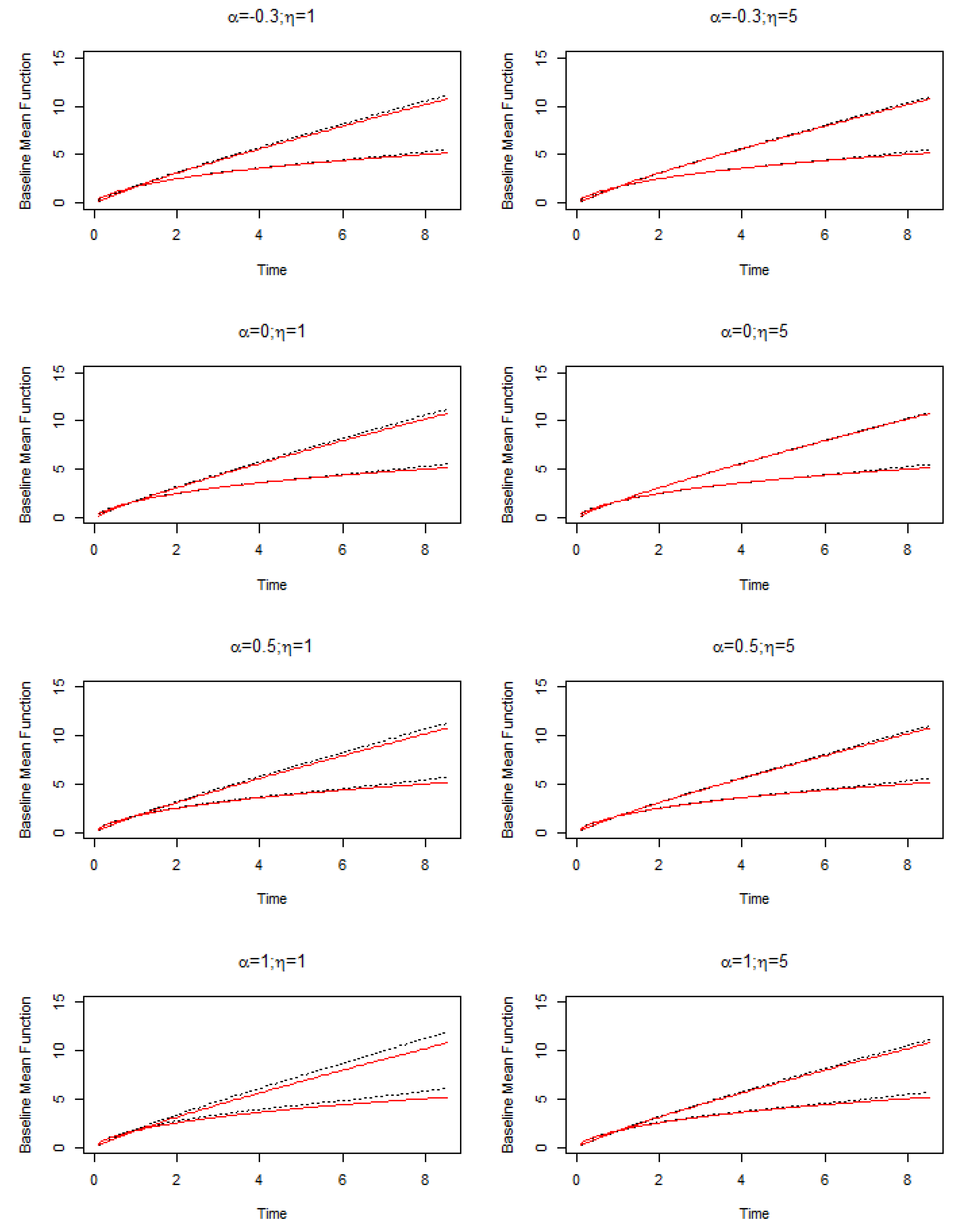
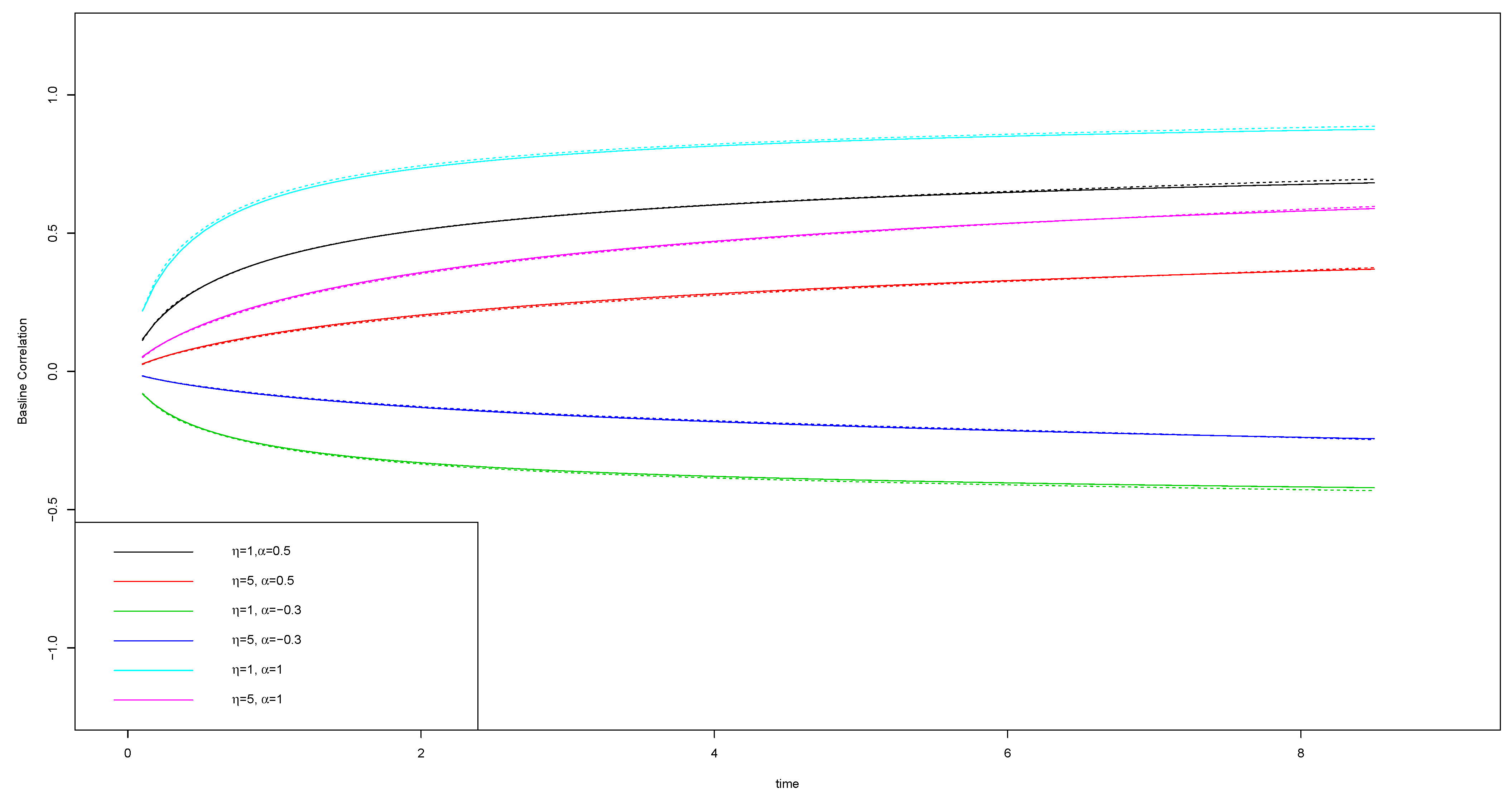
4.2. Simulation Results

We implemented the Gibbs sampler in Section 3.3 for each simulated dataset. Good mixing and fast convergence in the chains of the key parameters were observed. The convergence assessment was carried out using various convergence criteria in the R package coda [31]. The following results are summarized based on 5000 iterations of the Gibbs samples after discarding the first 2000 iterations as a burn-in.

The first set of simulations aims at assessing the performance of estimating regression coefficients ${\mathbf{\beta }}^{\left(k\right)}$. For this set of simulations, data are generated with different true $\beta$ values but $\alpha$ fixed at 1.

Table A1. Simulation results: estimation of regression coefficients from our proposed method when true $\alpha =1$. Bias refers to the difference between the average of the 500 posterior means and the true value; SD refers to the mean of the 500 posterior standard deviations; SE refers to the standard deviation of the 500 posterior means, and CP95 refers to the 95% coverage probability.

		$\mathit{\eta }=1$				$\mathit{\eta }=5$
Parameter	Truth	Bias	SD	SE	CP95	Bias	SD	SE	CP95
${\beta }_1^{\left(1\right)}$	0	0.0583	0.2238	0.1988	0.9520	0.0214	0.1287	0.1319	0.9400
${\beta }_2^{\left(1\right)}$	1	0.0004	0.1215	0.1223	0.9520	0.0015	0.0696	0.0722	0.9300
${\beta }_1^{\left(2\right)}$	1	0.0561	0.2225	0.1975	0.9700	0.0203	0.1291	0.1236	0.9600
${\beta }_2^{\left(2\right)}$	1	−0.0002	0.1203	0.1220	0.9480	0.0004	0.0683	0.0689	0.9460
${\beta }_1^{\left(1\right)}$	0	0.0392	0.2294	0.2179	0.9580	0.0178	0.1303	0.1311	0.9520
${\beta }_2^{\left(1\right)}$	1	−0.0053	0.1245	0.1228	0.9520	−0.0008	0.0714	0.0709	0.9520
${\beta }_1^{\left(2\right)}$	−1	0.0647	0.2523	0.2479	0.9560	0.0364	0.1651	0.1607	0.9500
${\beta }_2^{\left(2\right)}$	1	−0.0109	0.1344	0.1297	0.9620	−0.0001	0.0858	0.0824	0.9620
${\beta }_1^{\left(1\right)}$	1	0.0490	0.2198	0.2133	0.9500	0.0119	0.1203	0.1191	0.9540
${\beta }_2^{\left(1\right)}$	1	−0.0078	0.1182	0.1202	0.9280	−0.0017	0.0646	0.0653	0.9380
${\beta }_1^{\left(2\right)}$	−1	0.0771	0.2497	0.2373	0.9440	0.0400	0.1629	0.1593	0.9500
${\beta }_2^{\left(2\right)}$	1	−0.0127	0.1323	0.1335	0.9440	−0.0026	0.0840	0.0825	0.9600
${\beta }_1^{\left(1\right)}$	1	−0.0639	0.2152	0.2173	0.9320	−0.0178	0.1192	0.1194	0.9392
${\beta }_2^{\left(1\right)}$	−1	0.0025	0.1138	0.1121	0.9500	0.0051	0.0633	0.0678	0.9392
${\beta }_1^{\left(2\right)}$	1	−0.0663	0.2202	0.2247	0.9300	−0.0219	0.1280	0.1329	0.9196
${\beta }_2^{\left(2\right)}$	1	0.0031	0.1177	0.1156	0.9440	0.0046	0.0681	0.0786	0.9412

shows the estimation bias (Bias) defined as the average of the posterior means minus the true value, the mean of the posterior standard deviations (SD), standard deviation of the posterior means (SE), and 95% coverage probability (CP95) of four combinations of $\beta$ values. Clearly, the estimation of regression coefficients is good with small biases, SDs close to SEs, and 95% coverage probabilities around 95%. When $\eta$ goes from 1 to 5 (i.e., the variance of frailty goes from 1 to 0.2), the Bias, SD and SE uniformly become smaller. It is noted that the estimation of ${\beta }_2$ is consistently better than that of ${\beta }_1$ in terms of giving smaller biases and SDs and SEs. This is because that $X_2$ is a normal covariate providing more information than a binary covariate $X_1$, and that the variance of $X_2$ is four times the variance of $X_1$. Our simulation study shows that when we add one more possible value to $X_1$ such that $X_1$ follows a uniform discrete distribution with $X_1\in \{0,1,-1\}$, the estimation of ${\beta }_1$’s is improved and close to the estimation of ${\beta }_2$.

The second set of simulations focuses on assessing the estimation performance of our proposed methods when data are generated with different $\alpha$ values. The true $\beta$ values are fixed as ${\beta }_1^{\left(1\right)}=1$, ${\beta }_2^{\left(1\right)}=-1$, ${\beta }_1^{\left(2\right)}=1$, and ${\beta }_2^{\left(2\right)}=1$.

Table A2. Simulation results: estimation of regression coefficients $\alpha$ and $\eta$ from our proposed method for data generated with different $\alpha$ values and true ${\beta }_1^{\left(1\right)}=1$, ${\beta }_2^{\left(1\right)}=-1$, ${\beta }_1^{\left(2\right)}=1$, and ${\beta }_2^{\left(2\right)}=1$. Bias refers to the difference between the average of the 500 posterior means and the true value; SD refers to the mean of the 500 posterior standard deviations; SE refers to the standard deviation of the 500 posterior means, and CP95 refers to the 95% coverage probability.

		$\mathit{\eta }=1$				$\mathit{\eta }=5$
Parameter		Bias	SD	SE	CP95	Bias	SD	SE	CP95
$\alpha =-0.3$	${\beta }_1^{\left(1\right)}$	−0.0269	0.2190	0.2266	0.9300	−0.0124	0.1216	0.1252	0.9360
	${\beta }_2^{\left(1\right)}$	−0.0054	0.1168	0.1202	0.9460	0.0006	0.0652	0.0685	0.9460
	${\beta }_1^{\left(2\right)}$	−0.0086	0.1048	0.1049	0.9440	−0.0022	0.0829	0.0812	0.9540
	${\beta }_2^{\left(2\right)}$	0.0021	0.0548	0.0580	0.9400	0.0006	0.0421	0.0421	0.9600
	$\alpha$	−0.0083	0.0423	0.0462	0.9200	−0.0033	0.1010	0.1010	0.9400
	$\eta$	0.0412	0.1699	0.1754	0.9440	0.2494	1.0231	0.8814	0.9740
$\alpha =0$	${\beta }_1^{\left(1\right)}$	−0.0051	0.2229	0.2256	0.9400	−0.0017	0.1208	0.1175	0.9588
	${\beta }_2^{\left(1\right)}$	−0.0043	0.1195	0.1195	0.9460	−0.0004	0.0654	0.0682	0.9294
	${\beta }_1^{\left(2\right)}$	−0.0034	0.0758	0.0767	0.9460	−0.0048	0.0770	0.0749	0.9608
	${\beta }_2^{\left(2\right)}$	−0.0010	0.0370	0.0378	0.9580	0.0007	0.0377	0.0365	0.9627
	$\alpha$	0.0028	0.0344	0.0349	0.9420	0.0017	0.1152	0.1078	0.9784
	$\eta$	0.0328	0.1790	0.1781	0.9560	0.6264	1.3301	1.3349	0.9588
$\alpha =0.5$	${\beta }_1^{\left(1\right)}$	−0.0190	0.2194	0.2227	0.9360	−0.0076	0.1213	0.1179	0.9588
	${\beta }_2^{\left(1\right)}$	−0.0136	0.1162	0.1190	0.9340	0.0001	0.0647	0.0652	0.9490
	${\beta }_1^{\left(2\right)}$	−0.0263	0.1372	0.1338	0.9400	−0.0143	0.0958	0.0946	0.9549
	${\beta }_2^{\left(2\right)}$	−0.0047	0.0719	0.0697	0.9600	0.0010	0.0497	0.0475	0.9588
	$\alpha$	0.0066	0.0589	0.0578	0.9480	0.0163	0.1213	0.1246	0.9471
	$\eta$	0.0496	0.1729	0.1841	0.9500	0.4241	1.2655	1.2633	0.9569
$\alpha =1$	${\beta }_1^{\left(1\right)}$	−0.0639	0.2152	0.2173	0.9320	−0.0178	0.1192	0.1194	0.9392
	${\beta }_2^{\left(1\right)}$	0.0025	0.1138	0.1121	0.9500	0.0051	0.0633	0.0678	0.9392
	${\beta }_1^{\left(2\right)}$	−0.0663	0.2202	0.2247	0.9300	−0.0219	0.1280	0.1329	0.9196
	${\beta }_2^{\left(2\right)}$	0.0031	0.1177	0.1156	0.9440	0.0046	0.0681	0.0786	0.9412
	$\alpha$	0.0089	0.0804	0.0745	0.9760	0.0294	0.1529	0.1577	0.9392
	$\eta$	0.0469	0.1684	0.1734	0.9540	0.3745	1.2136	1.2777	0.9490

summarizes the estimation results. The estimation results of regression coefficients are similar as those in Table A1. Overall, the estimation is good with small biases, SDs close to SEs, and the CP95s close to 95%. The estimation is more precise for the larger $\eta$ value, and the estimation of ${\beta }_2$ is overall better than that of ${\beta }_1$. A new fact is observed that with the magnitude of $\alpha$ approaching 0, the estimation of the regression coefficients for the second type of event becomes more precise with smaller biases and SDs and SEs. This observation is reasonable, as the smaller value of $\alpha$ reflects the occurrence of the second type of events less affected by frailties, and thus the more precise estimation of the regression coefficients is expected. Furthermore, the estimated $\alpha$ and $\eta$ have remarkably caught the truth. Different from the estimation of regression coefficients, a small value of $\eta$ leads to the better estimation of $\alpha$. A glance at the table may find the bias of $\eta$ is a little too high when the true $\eta$ is 5. We need to point out that the difference between $\mathcal{G}(5,5)$ and $\mathcal{G}(6,6)$ is trivial, so the estimation can still accurately catch the shape of the distribution. Figure A2 shows the estimation of the baseline mean functions corresponding to different setups of $\alpha$ and $\eta$ values. The solid lines represent the real baseline mean function and the broken lines represent the estimated baseline mean function. The two lines on the top are for the first type of event $U_0^{\left(1\right)}\left(t\right)=t+log(1+t)$, and the curvilinear lines at the bottom are for the baseline mean function $U_0^{\left(2\right)}\left(t\right)=t^{0.5}+log(1+t)$ of the second type of event. We can clearly see that all the estimated lines catch up to the true lines well and the plots on the right side when $\eta =5$ show an even better convergence to the truth than their counterparts on the left side when $\eta =1$. Figure A3 shows the estimation of the baseline correlation functions corresponding to different setups of $\alpha$ and $\eta$ values. It is clear that for each $\alpha$ and $\eta$ setup, the estimated baseline correlation function overlays the true baseline correlation function.

Finally, we evaluate the effect of the scale parameter $\alpha$ on the estimation. Frailty models are well accepted for univariate panel count due to its flexibility and robustness. A naive extension to multivariate panel count data is to treat the frailty exactly the same for all types of events, i.e., each subject shares the common frailty to its full extent for all the events. Our simulation shows that this practice leads to wrong estimation results when true $\alpha$ is not 1.

Table A3. Simulation results: estimation of regression coefficients and $\eta$ from the naive method for data generated with different $\alpha$ values and true ${\beta }_1^{\left(1\right)}=1$, ${\beta }_2^{\left(1\right)}=-1$, ${\beta }_1^{\left(2\right)}=1$, and ${\beta }_2^{\left(2\right)}=1$. Bias refers to the difference between the average of the 500 posterior means and the true value; SD refers to the mean of the 500 posterior standard deviations; SE refers to the standard deviation of the 500 posterior means, and CP95 refers to the 95% coverage probability.

		$\mathit{\eta }=1$				$\mathit{\eta }=5$
Parameter		Bias	SD	SE	CP95	Bias	SD	SE	CP95
$\alpha =-0.3$	${\beta }_1^{\left(1\right)}$	−0.0438	0.1344	0.2443	0.7220	−0.0130	0.1016	0.1288	0.8640
	${\beta }_2^{\left(1\right)}$	0.0061	0.0710	0.1388	0.7080	0.0009	0.0536	0.0722	0.8500
	${\beta }_1^{\left(2\right)}$	−0.0206	0.1353	0.1628	0.8880	−0.0103	0.1085	0.0938	0.9800
	${\beta }_2^{\left(2\right)}$	0.0062	0.0715	0.0967	0.8540	0.0027	0.0574	0.0525	0.9720
	$\eta$	2.6937	0.6275	0.9058	0.0000	3.9252	0.8115	0.3937	0.0060
$\alpha =0$	${\beta }_1^{\left(1\right)}$	−0.0114	0.1459	0.2308	0.7820	−0.0046	0.1021	0.1205	0.9080
	${\beta }_2^{\left(1\right)}$	−0.0028	0.0770	0.1294	0.7700	0.0010	0.0544	0.0690	0.8760
	${\beta }_1^{\left(2\right)}$	−0.0302	0.1513	0.1166	0.9800	−0.0095	0.1106	0.0843	0.9900
	${\beta }_2^{\left(2\right)}$	0.0080	0.0802	0.0709	0.9820	0.0031	0.0587	0.0474	0.9780
	$\eta$	1.9095	0.4903	0.6390	0.0000	3.6761	0.9184	0.5119	0.0320
$\alpha =0.5$	${\beta }_1^{\left(1\right)}$	−0.0282	0.1826	0.2277	0.8840	−0.0059	0.1073	0.1185	0.9160
	${\beta }_2^{\left(1\right)}$	−0.0092	0.0962	0.1194	0.8780	−0.0002	0.0568	0.0646	0.9220
	${\beta }_1^{\left(2\right)}$	−0.0536	0.1893	0.1383	0.9760	−0.0193	0.1162	0.0962	0.9780
	${\beta }_2^{\left(2\right)}$	−0.0016	0.0997	0.0777	0.9880	0.0037	0.0617	0.0496	0.9920
	$\eta$	0.5948	0.2502	0.2712	0.2160	2.3688	1.1662	0.9781	0.4600
$\alpha =1$	${\beta }_1^{\left(1\right)}$	−0.0679	0.2161	0.2179	0.9320	−0.0181	0.1196	0.1194	0.9420
	${\beta }_2^{\left(1\right)}$	0.0029	0.1136	0.1118	0.9500	0.0027	0.0631	0.0614	0.9500
	${\beta }_1^{\left(2\right)}$	−0.0690	0.2202	0.2261	0.9380	−0.0208	0.1276	0.1315	0.9280
	${\beta }_2^{\left(2\right)}$	0.0022	0.1170	0.1155	0.9520	0.0019	0.0673	0.0702	0.9440
	$\eta$	0.0401	0.1552	0.1614	0.9400	0.1853	0.9692	0.9736	0.9600

presents the estimation results for the same simulated datasets as in Table A2, but are fitted with the naive model, i.e., model (1) with $\alpha$ omitted. The last block of rows of the table shows that the naive model does a comparable job in estimating the regression coefficients and $\eta$, which is reasonable because the naive model is the true model when the true value of $\alpha$ is 1. However, for other data generated with $\alpha$ not equal to 1, the misspecified naive model provides bad estimation results, which is especially clear when true $\eta =1$. Compared with the results in Table A2, all Biases for the regression coefficients slightly increase. For the regression coefficients for the first type of event, ${\beta }_1^{\left(1\right)}$ and ${\beta }_2^{\left(1\right)}$, the SEs are quite close to those in Table A2, but the SDs become smaller (the further away the true $\alpha$ is from 1, the smaller the SDs become), leading to CP95 being much smaller than 95%. For the regression coefficients for the second type of event, ${\beta }_1^{\left(2\right)}$ and ${\beta }_2^{\left(2\right)}$, compared with those in Table A2, both SDs and SEs increase. When data are generated with $\alpha =0$ or $0.5$, the naive method inflates SDs more than SEs, leading to higher coverage probabilities than 95%. When $\alpha =-0.3$, the inflated SEs are actually larger than the inflated SDs, leading to lower coverage probabilities. The bias, SD and SE of $\eta$ are increased when the true $\alpha$ gets away from the value 1. The estimation results for $\eta =5$ have a similar pattern to those for $\eta =1$ but much better, which is reasonable because the large $\eta$ value implies a small variance of frailties and thus less correlation between two types of events. This set of simulations shows that including the scale parameter of $\alpha$ is important to correctly estimate the regression coefficients.

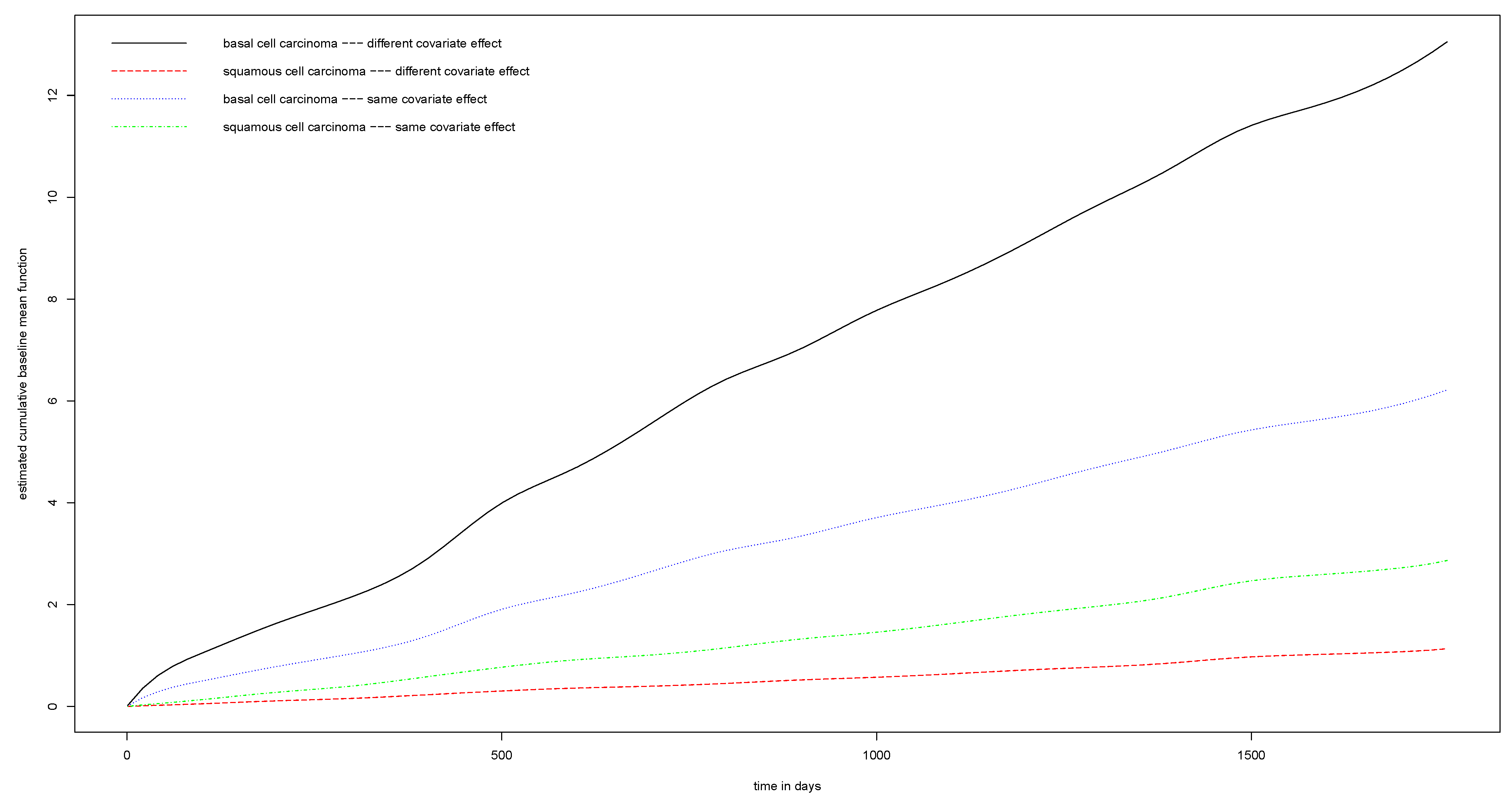
5. Real Data Analysis

In this section, we apply our proposed methods to analyze the motivating dataset, the skin cancer dataset, which was introduced in Section 1, and compare the results with those in the literature. Two hundred and ninety patients are analyzed, with one removed from the original group because of no observation. The observation times were recorded in days. The covariate of major interest is denoted as $X_1$, which is equal to 1 if the patient was assigned in the DFMO group and 0 in the placebo group. The other three covariates of interest are $X_2$, the number of cancers prior to the trial; $X_3$, the patient’s age; and $X_4$, gender with male 1 and female 0.

Table A4. Estimation results (posterior mean, posterior standard deviation and 95% credible interval) of the covariate effects for the two types of skin cancers. * indicates statistically significant.

	${\mathit{\beta }}_1$	${\mathit{\beta }}_2$	${\mathit{\beta }}_3$	${\mathit{\beta }}_4$
basal	−0.1902	0.1028	−0.0376	0.0238
	0.1500	0.0145	0.0055	0.1506
	(−0.4894, 0.0987)	(0.0762, 0.1330) *	(−0.0487, −0.0273) *	(−0.2717, 0.3185)
squamous	0.1055	0.1451	−0.0196	0.3053
	0.2174	0.0213	0.0070	0.2142
	(−0.3153, 0.5251)	(0.1051, 0.0.1894) *	( −0.0333, −0.0060) *	(−0.1165, 0.7255)

displays the results of the covariate coefficients of the two types of skin cancer from the proposed model. Clearly, gender ($X_4$) has no significant effect, but the number of cancers prior to trial ($X_2$) and the patient’s age ($X_3$) are significant for both skin cancers. The positive value of ${\beta }_2$ implies that the number of prior cancers has a positive relationship with the rate of new cancers. The negative value of ${\beta }_3$ suggests that older patients tend to have a lower recurrence rate of new cancers, which makes biological sense as older people have a slower metabolism. However, DFMO has different effects on the recurrence rate of the two skin cancers. For basal cell carcinoma, the recurrence rate is decreased by a factor of 1.209, but for squamous cell carcinoma, the recurrence rate is increased by a factor of 1.111. However, neither of these two effects are significant due to the large posterior standard deviations.

The skin cancer data have also been analyzed by He et al. [8] and Zhang et al. [9], assuming the same covariate effects for both skin cancers. For comparison, we also modify step 4 in the Gibbs sampler in Section 3.3 and reanalyze the data with the same covariate coefficients for both cancers. The results are presented in

Table A5. Estimation results (posterior mean, posterior standard deviation and 95% credible interval) of the covariate effects when common covariate effects are assumed for the two types of skin cancers from the proposed method, He et al. (2008)’s method, and Zhang et al. (2013)’s method. * indicates statistically significant.

	${\mathit{\beta }}_1$	${\mathit{\beta }}_2$	${\mathit{\beta }}_3$	${\mathit{\beta }}_4$
Proposed	−0.1509	0.0810	−0.0264	0.0636
	0.1381	0.0122	0.0052	0.1409
	(−0.4203, 0.1197)	(0.0599, 0.1087) *	(−0.0367, −0.0169) *	(−0.2098, 0.3369)
He et al.	−0.0239	0.1440	−0.0116	0.3807
	0.1809	0.0212	0.0084	0.1778
	(−0.3785, 0.3307)	(0.1024, 0.1856) *	(−0.0281, 0.0049)	(0.0322, 0.7292) *
Zhang et al.	−0.2253	0.0784	0.0016	0.2534
	0.1831	0.0090	0.0087	0.1942
	(−0.5842, 0.1336)	(0.0608, 0.0960) *	(−0.0155, 0.0187)	(−0.1272, 0.06340)

. Overall, all the estimation results of the covariate coefficients for the three methods assuming common covariate effects are quite similar, with the Bayesian method producing smaller posterior standard deviations of the regression coefficients than the standard errors from the other two frequentist methods. The different effects of DFMO on the two skin cancers are completely hidden compared to the method where different covariate effects are assumed. The effect of the number of cancers prior to trial ($X_2$) is significant for all three methods. Our Bayesian method shows the significant effect of patient’s age ($X_3$), while the other two frequentist methods do not. Our method and Zhang et al. [9]’s method show no significant effect of gender ($X_4$), but He et al. [8]’s method does.

Our methods can estimate the baseline mean functions simultaneously with the regression coefficients. Figure A4 presents the estimated baseline mean functions for basal cell carcinoma and squamous cell carcinoma, respectively. The solid line on the top and the broken line at the bottom represent the baseline mean functions of basal cell carcinoma and squamous cell carcinoma from the model, assuming different covariate effects. The two broken lines in the middle represent the baseline mean functions of the two cancers when assuming the covariate effects are the same. Clearly, under the common covariate effects assumption, the baseline mean functions are both pulled towards the middle, which blurs the difference of the mean functions between these two skin cancers.

Finally, Figure A5 displays the estimated baseline correlation function when covariate effects are assumed different for the two skin cancers. It shows that the correlation between the two recurrent skin cancers is positive and strengthened across time.

6. Discussion

In this paper, we have proposed a Bayesian estimation approach for the semiparametric regression analysis of multivariate panel count data. For each type of event, the proportional mean model is adopted to model the cumulative mean count of the event, where its baseline mean function is approximated by monotone I-splines. The correlation between multiple types of events is modeled by common frailty terms and scale parameters. Based on the novel Poisson data augmentation, an efficient and easy-to-implement Gibbs sampler is developed for the MCMC computation. Through the MCMC samples, the regression coefficients, the baseline mean functions, and the baseline correlation function can be simultaneously estimated. Simulation studies have shown that the proposed approach provides accurate estimation of the regression coefficients and the baseline mean functions. Simulation studies have also demonstrated the importance of including the scale parameter in the model. The scale parameter provides substantive flexibility for modeling the correlation and meanwhile improving the estimation performance.

Instead of using a single common frailty $w_i$ and scale parameters to model the correlation between counts of multiple events, another possible way is to have a frailty vector $(w_{i1},w_{i2},\dots ,w_{iK})$ for each subject. Then, the correlation between counts of multiple events is modeled through the dependence structure of these $w_{ij}$s. Bedair et al. [32] used copula-frailty models to analyze correlated recurrent events of different types. We may also borrow the copula-frailty idea to more flexibly model the correlation between counts of multiple events. In this paper, we assume frailties follow a gamma distribution $\mathcal{G}(\eta ,\eta )$. The gamma frailty is the simplest and most popular frailty distribution in survival analysis. Under the mean equal to 1 restriction, there is only one parameter $\eta$ to represent the variance in the frailty, which is easy to interpret when connecting to the correlation. Some other frailties may also be used, such as log normal frailty and inverse Gaussian frailty. Then, the formula for the correlation and the sampling for the frailty would be different. Other possible choices of frailties are referred to by Balan and Putter [33], who provide an excellent tutorial on frailty models.

Regarding choosing which event as the reference event, in this paper, we choose the event with the largest frailty variability as the reference event. One possible way to choose the reference event is to first conduct univariate panel count data analysis for each type of event, and then to choose the one with the largest frailty variability as the reference event. For real data analysis, gamma frailty assumption may not hold for the reference event. For this, nonparametric frailties without assuming any specific distribution may be a more flexible choice.

Our approach can be slightly modified to accommodate common covariate effects for different types of events. However, the real data analysis shows that doing this would hide significant covariate effects for individual types of events. Therefore, we suggest assuming different covariate effects for different events first for real data analysis and then using the common covariate effect model later if similar effects are observed for different events.

Unlike the existing frequentist methods, our approach does not require model assumptions for the observation or censoring processes. Our approach is solely based on the observed likelihood and only needs the observed counts and observation times for the analysis, which makes our proposed approach generic to deal with panel count data arising from different observation schemes, including dependent or independent censoring and/or observation processes. On the other hand, the proposed approach may lose a certain amount of efficiency due to not incorporating the information of the observation or censoring processes when they are actually available.

References

1. Sun, J.; Zhao, X. Statistical Analysis of Panel Count Data; Springer: Berlin/Heidelberg, Germany, 2013. [Google Scholar]
2. Sun, J.; Kalbfleisch, J. Estimation of the mean function of point processes based on panel count data. Stat. Sin. 1995, 5, 279–289. [Google Scholar]
3. Wellner, J.A.; Zhang, Y. Two estimators of the mean of a counting process with panel count data. Ann. Stat. 2000, 28, 779–814. [Google Scholar] [CrossRef]
4. Wellner, J.A.; Zhang, Y. Two likelihood-based semiparametric estimation methods for panel count data with covariates. Ann. Stat. 2007, 35, 2106–2142. [Google Scholar] [CrossRef] [Green Version]
5. Lu, M.; Zhang, Y.; Huang, J. Estimation of the mean function with panel count data using monotone polynomial splines. Biometrika 2007, 94, 705–718. [Google Scholar] [CrossRef] [Green Version]
6. Lu, M.; Zhang, Y.; Huang, J. Semiparametric estimation methods for panel count data using monotone B-splines. J. Am. Stat. Assoc. 2009, 104, 1060–1070. [Google Scholar] [CrossRef]
7. Wang, J.; Lin, X. A Bayesian approach for semiparametric regression analysis of panel count data. Lifetime Data Anal. 2020, 26, 402–420. [Google Scholar] [CrossRef]
8. He, X.; Tong, X.; Sun, J.; Cook, R.J. Regression analysis of multivariate panel count data. Biostatistics 2008, 9, 234–248. [Google Scholar] [CrossRef]
9. Zhang, H.; Zhao, H.; Sun, J.; Wang, D.; Kim, K. Regression analysis of multivariate panel count data with an informative observation process. J. Multivar. Anal. 2013, 119, 71–80. [Google Scholar] [CrossRef]
10. Li, N.; Park, D.H.; Sun, J.; Kim, K. Semiparametric transformation models for multivariate panel count data with dependent observation process. Can. J. Stat. 2010, 39, 458–474. [Google Scholar] [CrossRef] [Green Version]
11. Zhao, H.; Li, Y.; Sun, J. Semiparametric analysis of multivariate panel count data with dependent observation processes and a terminal event. J. Nonparametr. Stat. 2013, 25, 379–394. [Google Scholar] [CrossRef]
12. He, X.; Feng, X.; Tong, X.; Xingqiu, Z. Semiparametric partially linear varying coefficient models with panel count data. Lifetime Data Anal. 2017, 23, 439–466. [Google Scholar] [CrossRef] [PubMed]
13. Zhao, H.; Zhang, Y.; Zhao, X.; Yu, Z. A nonparametric regression model for panel count data analysis. Stat. Sin. 2019, 29, 809–826. [Google Scholar] [CrossRef] [Green Version]
14. Wang, Y.; Yu, Z. A kernel regression model for panel count data with time-varying coefficients. arXiv 2019, arXiv:1903.10233. [Google Scholar] [CrossRef]
15. Li, Y.; He, X.; Wang, H.; Zhang, B.; Sun, J. Semiparametric regression of multivariate panel count data with informative observation times. J. Multivar. Anal. 2015, 140, 209–219. [Google Scholar] [CrossRef]
16. Wang, Y.; Yu, Z. A kernel regression model for panel count data with nonparametric covariate functions. Biometrics 2021. [Google Scholar] [CrossRef]
17. Chib, S.; Greenberg, E.; Winkelmann, R. Posterior simulation and Bayes factors in panel count data models. J. Econom. 1998, 86, 33–54. [Google Scholar] [CrossRef] [Green Version]
18. Ramsay, J. Monotone regression splines in action. Stat. Sci. 1988, 3, 425–441. [Google Scholar] [CrossRef]
19. Dimitrakopoulos, S. Bayesian Estimation of Panel Count Data Models: Dynamics, Latent Heterogeneity, Serial Error Correlation, and Nonparametric Structures. Panel Data Econom. 2019, 6, 147–173. [Google Scholar]
20. Liang, Y.; Li, Y.; Zhang, B. Bayesian nonparametric inference for panel count data with an informative observation process. Biom. J. 2018, 60, 583–596. [Google Scholar] [CrossRef] [Green Version]
21. Sun, J.; Tong, X.; He, X. Regression analysis of panel count data with dependent observation times. Biometrics 2007, 63, 1053–1059. [Google Scholar] [CrossRef]
22. Sinha, D.; Maiti, T. A Bayesian approach for the analysis of panel-count data with dependent termination. Biometrics 2004, 60, 34–40. [Google Scholar] [CrossRef] [PubMed]
23. Lin, X.; Cai, B.; Wang, L.; Zhang, Z. A Bayesian proportional hazards model for general interval-censored data. Lifetime Data Anal. 2015, 21, 470–490. [Google Scholar] [CrossRef] [PubMed]
24. Cai, B.; Lin, X.; Wang, L. Bayesian proportional hazards model for current status data with monotone splines. Comput. Stat. Data Anal. 2011, 55, 2644–2651. [Google Scholar] [CrossRef]
25. Wang, L.; Dunson, D.B. Semiparametric Bayes’ Proportional Odds Models for Current Status Data with Underreporting. Biometrics 2011, 67, 1111–1118. [Google Scholar] [CrossRef] [Green Version]
26. Green, P.J. Reversible Jump Markov Chain Monte Carlo Computation and Bayesian Model Determination. Biometrika 1995, 82, 711–732. [Google Scholar] [CrossRef]
27. Park, T.; Casella, G. The Bayeisan Lasso. J. Am. Stat. Assoc. 2008, 103, 681–686. [Google Scholar] [CrossRef]
28. Gilks, W.R.; Wild, P. Adaptive rejection sampling for Gibbs sampling. Appl. Stat. 1992, 41, 337–348. [Google Scholar] [CrossRef]
29. Gilks, W.R.; Best, N.; Tan, K. Adaptive rejection Metropolis sampling within Gibbs sampling. Appl. Stat. 1995, 44, 455–472. [Google Scholar] [CrossRef] [Green Version]
30. Petris, G.; Tardella, L. Original C code for ARMS by Wally Gilks. HI: Simulation from Distributions Supported by Nested Hyperplanes. R Package Version 0.4. 2013. Available online: https://rdrr.io/cran/HI/ (accessed on 10 January 2022).
31. Plummer, M.; Best, N.; Cowles, K.; Vines, K. CODA: Convergence Diagnosis and Output Analysis for MCMC. R News 2006, 6, 7–11. [Google Scholar]
32. Bedair, K.F.; Hong, Y.; Al-Khalidi, H.R. Copula-frailty models for recurrent event data based on Monte Carlo EM algorithm. J. Stat. Comput. Simul. 2021, 91, 3530–3548. [Google Scholar] [CrossRef]
33. Balan, T.; Putter, H. A tutorial on frailty models. Stat. Methods Med. Res. 2020, 29, 3424–3452. [Google Scholar] [CrossRef] [PubMed]
Publisher’s Note: MDPI stays neutral with regard to jurisdictional claims in published maps and institutional affiliations.