Article

Exploring Heterogeneity with Category and Cluster Analyses for Mixed Data

1
European Centre for Living Technology (ECLT), Ca’ Foscari University of Venice, 30123 Venice, Italy
2
Department of Economic Sciences, Università del Salento, 73100 Lecce, Italy
3
Department of Engineering, University of Palermo, 90128 Palermo, Italy
*
Author to whom correspondence should be addressed.
Stats 2023, 6(3), 747-762; https://doi.org/10.3390/stats6030048
Submission received: 23 May 2023 / Revised: 29 June 2023 / Accepted: 1 July 2023 / Published: 5 July 2023

Abstract

:
Precision medicine aims to overcome the traditional one-model-fits-the-whole-population approach that is unable to detect heterogeneous disease patterns and make accurate personalized predictions. Heterogeneity is particularly relevant for patients with complications of type 2 diabetes, including diabetic kidney disease (DKD). We focus on a DKD longitudinal dataset, aiming to find specific subgroups of patients with characteristics that have a close response to the therapeutic treatment. We develop an approach based on some particular concepts of category theory and cluster analysis to explore individualized modelings and achieving insights onto disease evolution. This paper exploits the visualization tools provided by category theory, and bridges category-based abstract works and real datasets. We build subgroups deriving clusters of patients at different time points, considering a set of variables characterizing the state of patients. We analyze how specific variables affect the disease progress, and which drug combinations are more effective for each cluster of patients. The retrieved information can foster individualized strategies for DKD treatment.

1. Introduction

Precision medicine aims to find the best individualized treatment for each patient or a specific subgroup of patients [1,2]. To this aim, the analysis of patient heterogeneity with respect to a disease progress is a crucial step [3]. Recent developments of statistical and computational methods for precision medicine concern Q-learning [4], Markov chains [5], and cluster analysis [2].
Among computational tools, cluster analysis plays a key role, identifying subgroups of similar patients [6,7], investigating risk factors within each subgroup [8], and analyzing the heterogeneity of patients’ response to the therapeutic treatments [9]. In particular, cluster analysis was recently adopted to study type 2 diabetes [10], chronic kidney disease (CKD) patients [11], and diabetic kidney disease (DKD) patients [12].
In this paper, we focus on DKD patients [13]. We investigate the dissimilarity between patients at different time points, evaluating how it changes through time, and analyzing the response of patients to the given therapeutic treatment. We then build dissimilarity matrices (distance matrices) to compare different states of the patients. We compute distances of distances matrices to find out how the dissimilarity changes through time. This idea of nested distances can be formalized through transformations of transformations, which is the starting point of category theory [14,15]. We develop a category theory-inspired approach to formalize the construction of population subgroups and describe patterns of evolution. In this article, we use the language of categories to provide a diagrammatic representation of the different steps of our research.
Category theory counts recent developments in several fields of science, such as physics [16], chemistry [17], biology [18,19], and neuroscience [20]. It has also been applied to visualize the general idea of clustering, as a mapping from a dataset equipped with a distance to a set of partitions with distances [21]. This research is related to other formalization works [22,23]. This study contributes to bridging between abstract research clustering methods with real datasets. It provides the basic categorical language and the path to formalization, from dataset values and distances, to clusters’ nested comparisons. The novelty of our research is the development of a methodological approach based on the language of category theory and cluster analysis for a precision medicine problem.
In this research, we describe patients with mixed-type variables, and for this reason, we evaluate the dissimilarity between patients using the Gower distance [24,25,26]. Then, we compute dissimilarity matrices at consecutive time points based on these distances, and we build clusters of similar patients through hierarchical clusters using the Ward linkage method. We analyze the heterogeneity in the patients’ response to the treatment.
As results of this study, we find an increase in the heterogeneity of DKD patients through time, and we retrieve information about the effect of drug combinations for the different subgroups of patients. The current research is a development from a preliminary study [27] where the approach was sketched.
The structure of this article is the following. In Section 2, we build computational methods for assessing heterogeneity in patients’ response to the therapeutic treatment. In Section 3, we present the achieved results. In Section 4, we discuss the longitudinal aspect in our study and we summarize the research results in light of the categories.

2. Methodology

To address the heterogeneity of the DKD patients’ response to the therapeutic treatment, we develop a methodology based on some concepts of category theory (Section 2.1) and on the construction of clusters of similar patients (Section 2.2). We use the Gower distance (Section 2.2) to build distance matrices, evaluating the dissimilarity between each pair of patients, analyzing the heterogeneity of patients at different time points and through time. Then, we build hierarchical dendrograms using the Ward linkage method (Section 2.2). We evaluate the variation of dissimilarity matrices between consecutive time points to observe the main changes of heterogeneity across time.

2.1. Morphisms and Functors from Category Theory

To develop our approach based on the similarities between pairs of patients and pairs of matrices, we introduce basic definitions and graphic tools from category theory. Concepts of category theory are used here to formalize the idea of distances between patients characterized by a high number of variables, and of distances between distances as transformations. We start with some essential definitions, presenting values and distances as a category.
A category comprises objects (points) and the morphisms (arrows) between them. The composition of morphisms is associative, and there exists the identity morphism. A functor is a morphism between categories. It maps objects and morphisms of a category into objects and morphisms of another category, preserving structures. A natural transformation is a map between functors.
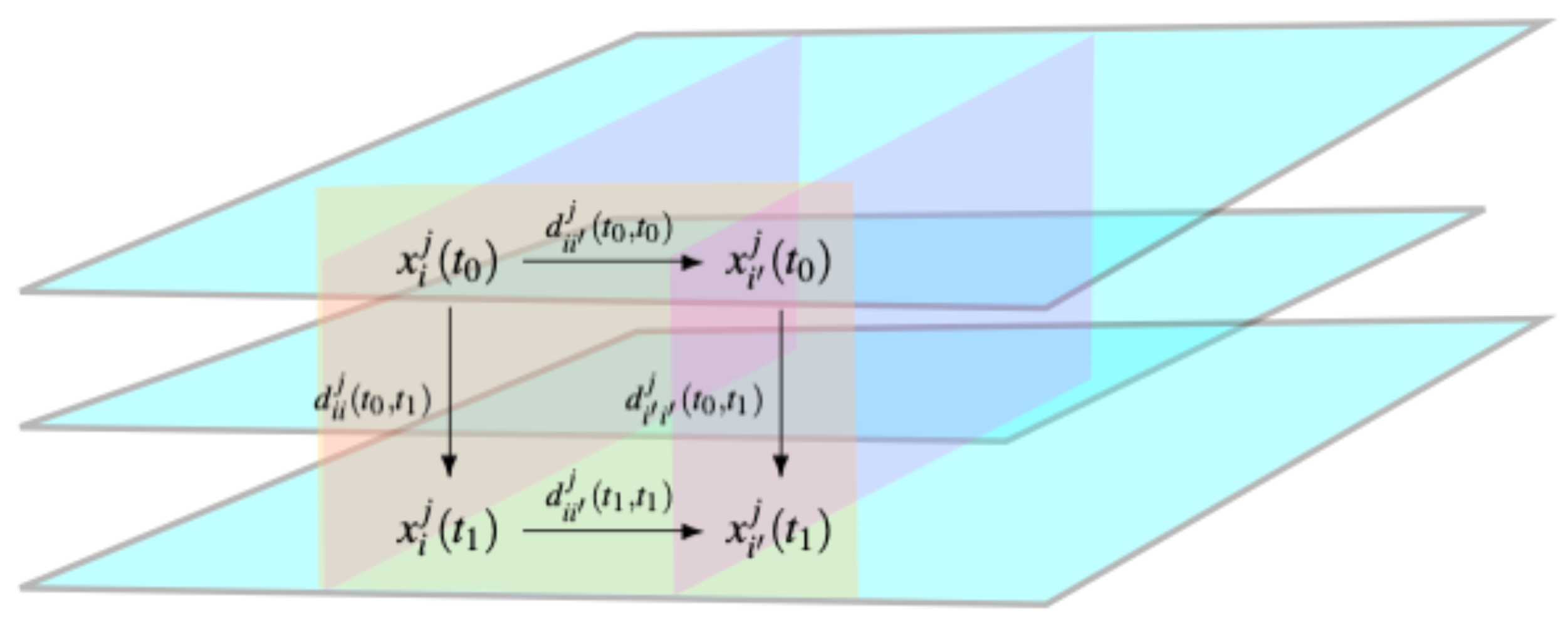
To contextualize objects and morphisms in our case study, we present the following representation of the dataset with n patients, p variables, and three time points t 0 , t 1 , t 2 . Each element is the observation x i j ( t k ) , where we have the following:
  • i indicates the patient, i = 1 , , n ;
  • j indicates the variable, j = 1 , , p ;
  • k indicates the time point, k = 0 , 1 , 2 .
We consider three time points: t 0 (the baseline), and t 1 and t 2 (the first and second follow-ups, respectively). We define two notions of distances: distance d i , i j ( t k , t k ) between observations of variable j at time k for patients i , i = 1 , , n ; distance d i , i j ( t k , t k ) between observations of patient i with respect to the values of variable j at different times k , k = 0 , 1 , 2 .
In terms of category theory, we can describe observations and distances as an enriched double category with metrics in R [15], whose objects are the values x i j ( t k ) and whose morphisms are vertical and horizontal distances. In fact, the values of the j-th variable (for all patients, for all times) are the objects, and distances between patients and distances between times are the morphisms. The properties of double categories are the object of recent theoretical studies [28,29].
In our research, the i-th patient at each time point t k is characterized as a triplet:
( x i ( t k ) , D ( t k ) , y i ( t k + 1 ) ) ,
where x i ( t k ) is the vector of the p variables
x i ( t k ) = [ x i 1 ( t k ) , x i 2 ( t k ) , , x i p ( t k ) ] ,
D ( t k ) = [ D 1 ( t k ) , D 2 ( t 1 ) , D 3 ( t k ) , D 4 ( t k ) ]
is the vector of the prescribed drugs, and y i ( t k + 1 ) is the value of the response variable Y at t k + 1 , which can be considered a measure of the effect of the drug given at t k .
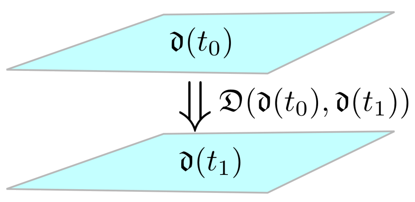
The diagram in (1) shows distances of the patients i , i at times t 0 , t 1 for the variable j. The horizontal composition shows comparisons between patients at the same time; vertical composition shows comparisons of the same patient through time. We can build lattices for each variable. Relationships between variables are formalized through mappings.
Stats 06 00048 i001
Mappings between variables can be formalized as functors. In fact, the structure of values/distances for one variable corresponds to the structure of values/distances for another variable. The identity property is represented by the zero distance of the same variable measured at the same time for the same patient.
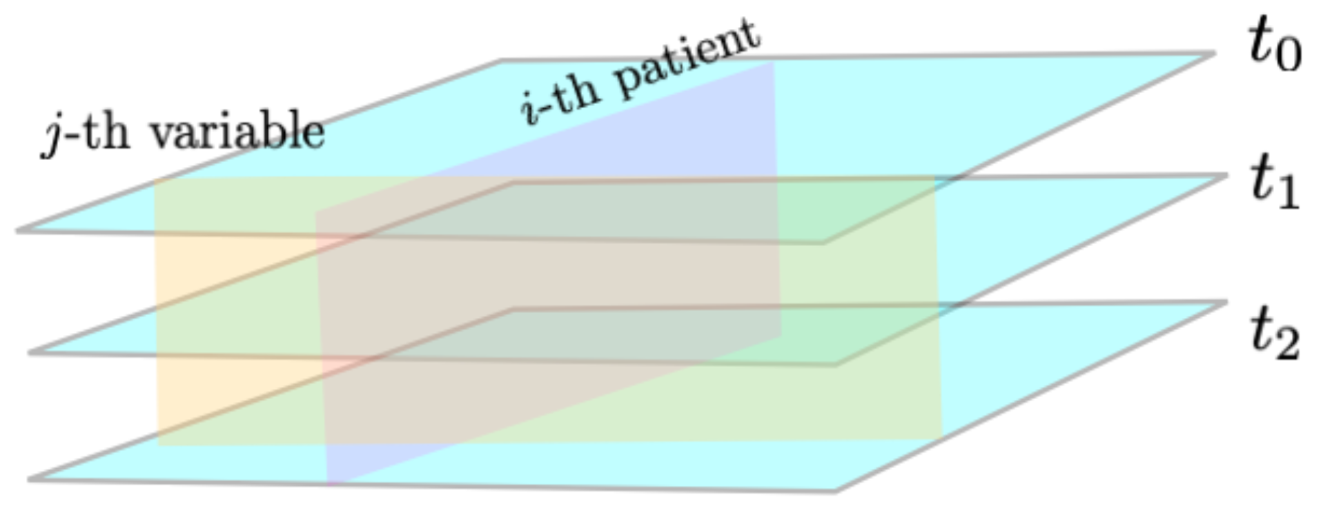
To compare pairs of patients with respect to all the variables we select, we encode this information in a value computing the Gower distance (Figure 1), as described in Section 2.2. Comparing patients pairwise at a given time point, we obtain a coefficient of similarity s [ 0 , 1 ] for each pair, where 1 stands for maximal similarity. To obtain the dissimilarity, we evaluate ( 1 s ) , where 1 stands for maximal dissimilarity. These so-obtained values constitute the elements of the dissimilarity matrix at a time point, d ( t k ) = | d i , i j ( t k , t k ) | i , i = 1 , , n , j = 1 , , p , k , k = 0 , , 2 . It is a symmetric matrix whose trace is zero. To find subgroups of similar patients, we build clusters using hierarchical dendrograms with the Ward distance (Section 2.2). We then evaluate inter-cluster and intra-cluster distances at different time points.
Evaluating different clustering methods, we obtain clusters with similar size and population characteristics. Adopting the language of category theory, the comparison between clustering methods [30] can be formalized through natural transformations [15,21].
To better describe our results, we consider two mathematical tools, the Frobenius norm and the Chebyshev distance.
To evaluate the heterogeneity of dissimilarity matrices d ( t k ) at each time point k = 1 , 2 , 3 , we compute their Frobenius norm, measuring the “variability” (interpreted as the size of the elements) of the matrix. The Frobenius norm takes as input a matrix, and gives as output a number, characterizing the overall size of the matrix elements. Given the squared matrix d ( t k ) R n × n , the Frobenius norm is defined as a squared L 2 norm:
d ( t k ) F = i = 1 n i = 1 n d ( t k ) i , i 2 = T r d ( t k ) d ( t k ) T ,
where T r is the trace of the matrix and T indicates the transposed matrix.
To evaluate the variation between matrices at two different time points, we compute the Chebyshev distance of d ( t 0 ) , d ( t 1 ) and of d ( t 1 ) , d ( t 2 ) . The Chebyshev distance between two matrices at different time points takes as input the two matrices and gives as output a number. If the two matrices are identical, the number is zero. The Chebyshev distance of two n × n matrices d ( t k ) , d ( t k + 1 ) is computed as follows:
d C ( d ( t k ) , d ( t k + 1 ) ) = m a x i , i [ [ 1 , n ] ] ( | d ( t k ) i , i d ( t k + 1 ) i , i | ) .

2.2. Hierarchical Clustering Based on Gower Distance

Cluster analysis is an unsupervised method with the aim to identify groups of similar patients according to a set of particular criteria. In this paper, we consider the agglomerative hierarchical clustering approach for a set of patients, considering their main clinical and sociodemographic characteristics related to risk factors [31,32]. The structure of this clustering approach can be summarized as follows. Initially each observation is considered as an individual cluster and then, at each step, the most similar pair of clusters are merged [33,34].
The notion of similarity between two objects is central in this work and implies a notion of distance. In particular, the concept of similarity between two objects implies a notion of distance between clusters and also a notion of distance between pairs of observations. The similarity between clusters is generally measured by linkage methods. In this study, we consider Ward-type linkage [35] for its good performance shown in several studies for clinical data clustering [36]. This linkage defines the distance between two clusters as the minimum within-cluster variance (minimum within-cluster inertia). In the hierarchical clustering, at each step, the two clusters with minimum within-cluster inertia are merged [37,38].
We measure the similarity of n observations according to the Gower distance [25], suitable for mixed-type qualitative and quantitative data. In our case study, we compute Gower-based distance matrices for each time point. The Gower distance gives a measure of similarity between the i-th and the i -th patients, based on all p variables that characterize the patient (Figure 2 and Figure 3). It is visually represented in Figure 1.
To precisely describe it, we consider patients characterized by a collection of values of mixed variables. To compare pairs of patients with continuous, binary, and ordinal variables, we compute the Gower distance with the Podani extension [24,25,26]. To build the Gower distance at a given time point, we start with its constitutive elements [26]. The similarity s j between two patients with respect to one variable takes a different form, according to its typology:
  • Quantitative variable: s j ( x i j , x i j ) = 1 | x i j x i j | R j , where R j is the observed range of variable j;
  • Nominal variable: s j ( x i j , x i j ) = 1 if patients i , i have the same value of the j-th variable at a given time, and 0 otherwise;
  • Ordinal variable: s j ( x i j , x i j ) = 1 | r j ( x i j ) r j ( x i j ) | r j ( x i * j ) r j ( x i j ) , where r is the rank of each measurement, i * is the patient having the highest rank of variable j, and i is the patient having the lowest rank of variable j. This is the Podani extension of the Gower formula [24], to include ordinal variables.
The Gower distance is thus defined as
d G ( i , i ) = 1 j = 1 p s j ( x i j , x i j ) δ j ( x i j , x i j ) j = 1 p δ j ( x i j , x i j ) ,
where δ j ( x i j , x i j ) takes the value of 0 if i or i have a missing value for the j-th variable, and otherwise takes the values of 1.
Then, we compute the pairwise distances between all patients and, with this information, we build the dissimilarity matrix, whose elements are d G ( i ( t k ) , i ( t k ) ) . We indicate the dissimilarity matrices as d ( t 0 ) , d ( t 1 ) , d ( t 2 ) . Starting from these matrices, we compute the matrices of distances of distances as D ( d ( t k ) , d ( t k + 1 ) ) = d ( t k + 1 ) d ( t k ) .

3. Results

3.1. The Case Study

We analyze a longitudinal dataset, the DC-ren dataset, from the project Drug combinations for rewriting trajectories of renal pathologies in type II diabetes (DC-ren)https://dc-ren.eu/ (accessed on 1 December 2020). The dataset consists of n = 235 diabetic kidney disease (DKD) patients, characterized by p = 10 mixed-type variables, of which 6 are continuous, 1 nominal and 3 binary. The continuous variables are serum triglycerides, body mass index (BMI), diastolic pressure, glycated hemoglobin (HbA1c), the ratio of urine albumin to creatinine (UACR), and the estimated glomerular filtration rate (eGFR). The nominal variables are serum potassium, mean arterial pressure, blood glucose, and C-reactive protein (CRP). The mean values of these variables for this population are listed in Table 1. These variables were measured at each time point for all patients, and they are described in detail in the Appendix A.
The patients are observed at three data points, t 0 , t 1 , t 2 , considering yearly visits. On these data, we build clusters at each time point. Our dataset does not contain missing data.
The population, constituted by 54% women and 46% men, has a mean age of 65.32 ± 8.9 years. The mean age of diabetes diagnosis and hypertension diagnosis for the considered patients is 51.7 ± 10.8 and 49.6 ± 12 respectively. The mean value of the difference between the year of type 2 diabetes diagnosis and the year of birth is 15 ± 10 years, and the mean value of the difference between the year of hypertension diagnosis and the year of birth is 13 ± 7 years. Of the patients, 53.2% never smoked, while the remaining patients include current smokers (11.1%) and ex-smokers (35.7%). Smoking constitutes a risk factor for renal and cardiovascular diseases.

3.2. Distances and Clusters of Patients

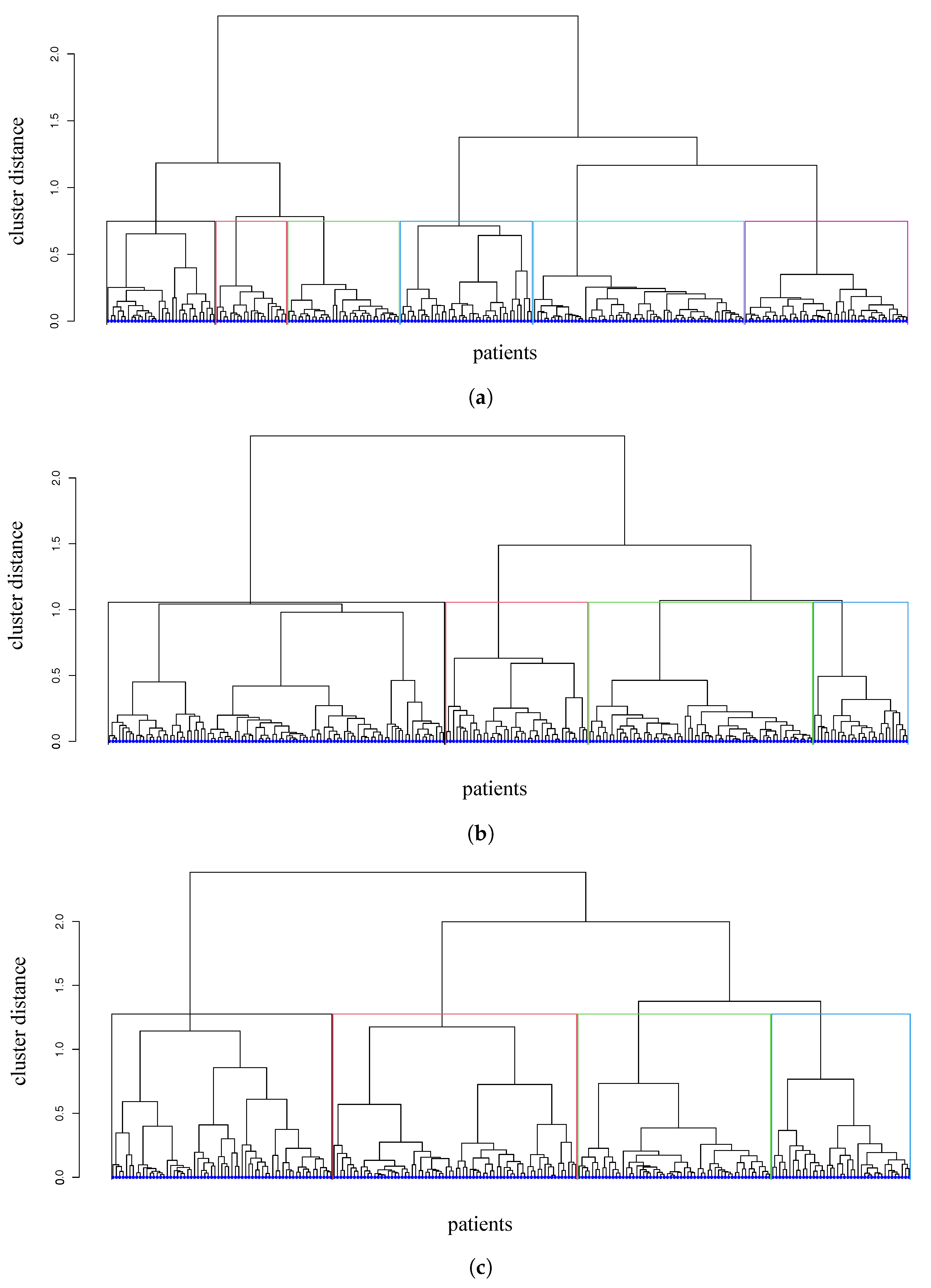
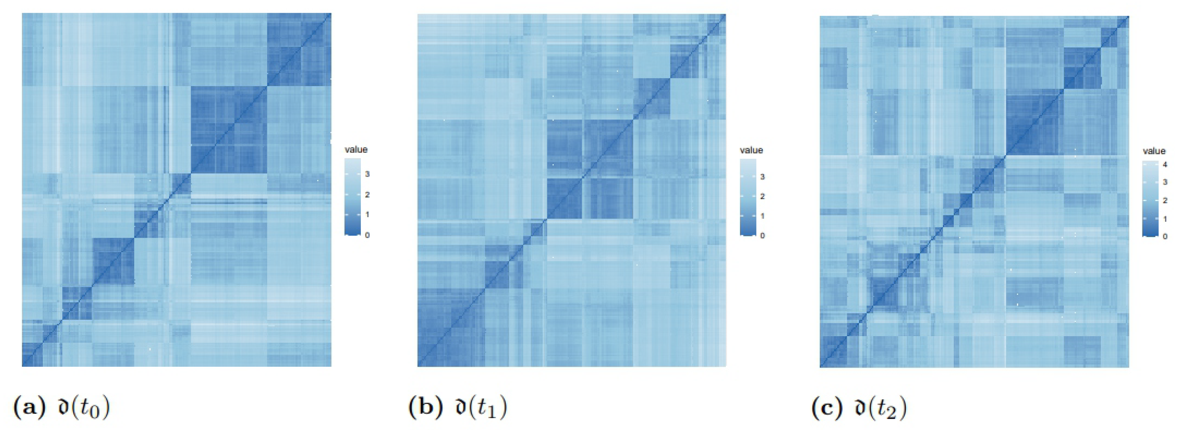
To verify if patients in similar conditions received similar drugs and to analyze their response to the therapeutic treatment, we evaluate their distances in terms of a set of variables and we build clusters of patients. To analyze the progressive evolution of the disease, we build hierarchical dendrograms (Figure 4). Computing the Gower distance at each time point, we obtain information regarding the presence of clusters (latent clusters). A visual inspection of matrices in Figure 5 reveals the presence of separated blocks. In order to computationally confirm this information, we then run a test assessing the probability of dealing with a randomly generated dataset. The test values range from 0 for low clusterability to 1 indicating the high clusterability of the data. For our dataset, the test returns the values of 0.92 at t 0 , 0.86 at t 1 , and 0.82 at t 2 , confirming the clusterability.
We build clusters through a three-step procedure: we estimate the best number of clusters, we find the best linkage method, and we derive the cluster distribution.
To find the optimal number of clusters at each time point, we adopt the method by Aschenbruck [39], which is suitable for mixed-type data. As the best number of clusters, we achieve 6 at t 0 and 4 at t 1 and 4 at t 2 . The number of clusters decreases through time not because of a diminution of the heterogeneity (that is actually increasing) but because the inter- and intra-variability of the clusters is increased (Table 2). Based on the above, we find that the Ward linkage method applied to these data is the best linkage clustering technique. We then derive clusters based on the Gower distance and Ward linkage method.
Distances in each dissimilarity matrix, inter-cluster distance, intra-cluster distance, and Frobenius norms at each time point are presented in Table 2. These indicators show an increase in heterogeneity, with a larger jump between t 1 and t 2 . Cluster validity measures and the characteristics of patients in each cluster are presented in Table 2 and Table 3.
We now investigate which patients are in each single cluster, and how they are moving through clusters over time, analyzing the triplet of variables, drugs, and response to the treatment. These results show a relation among the characteristics of the patients, the prescribed treatments, and the response to the given treatments. We comment the quantitative information on single variables according to precise medical taxonomies.
In this research, the target characteristic is the eGFR value, where the value of 60 mL/min/1.73 m 2 is considered the threshold for a sufficient kidney efficiency.
With respect to the therapeutic prescriptions, all patients were treated with RASi; some of them received an additional drug: SGLT2i, MCRa, or GLP1a. The action of each drug is summarized in Appendix A.
With this information, we obtain an overview of the degree of disease of patients in each cluster. Our comments take mainly into account eGFR, UACR, and HbA1c levels, variables that provide information on disease severity.
Time point t 0 . At t 0 we obtain six clusters, populated by patients with different degrees of disease, ranging from moderate to severe. The average of the within-distance [40] for all clusters is 0.11 [41,42], well below the average distance between clusters (0.25, Table 2). The averages of within-cluster distances for each cluster at each time point, and the values for each variable in every cluster of patients, are reported in Table 3. Clusters 1, 2, and 3 contain patients with mean values of eGFR above 60 mL/min/1.73 m 2 and mean value UACR below 72, indicating moderate disease [43]. However, these patients present high values of triglycerides (higher than 200) and BMI (higher than 31), indicating a cardiovascular risk connected with kidney complications. Patients in cluster 4 have a mean value of UACR of 89, indicating more significant disease. Patients in cluster 5 have a mean value of eGFR of 61 mL/min/1.73 m 2 , slightly above the threshold, but a lower average value of UACR (50.90) and a lower HbA1c (6.87), denoting better kidney efficiency. Moreover, patients in clusters 4 and 5 have the lowest triglycerides (143) and BMI values (30) compared with those in other clusters; therefore, these patients have minimal kidney risk related to life style and metabolism. Concerning the therapeutic treatment, most patients received only RASi.
Time point t 1 . At t 1 we find four clusters of patients. The average distance between clusters increases from the value 0.25 at t 0 to the value 0.27 at t 1 ; the average within-cluster distance rises from 0.11 to 0.14 (Table 2). While at t 0 the lowest mean eGFR value is 61.41 mL/min/1.73 m 2 , at t 1 , it is 56.71 mL/min/1.73 m 2 . For these patients, the low eGFR value is related to the highest mean value of BMI (34.07) and the highest level of triglycerides (238.32), connected with metabolism and cardiovascular risk, and with the highest mean value of HbA1c (8.22), related to glucose metabolism; however, these patients also present a low UACR (34.72), indicating lower kidney risk. This information confirms the possibility of the high risk of diabetic complications in spite of low HbA1c values [44]. Patients with a moderate disease are predominantly found in cluster 3; they have the highest mean eGFR value (65.71) at t 1 , and the lowest HbA1c (6.72), BMI (30.72), and triglycerides (154.08). For these patients, the kidney efficiency is well above the threshold (mean eGFR equal to 65.71 mL/min/1.73 m 2 , low mean UACR equal to 46.43), and the risk factors connected with lipid metabolism (indicated by triglycerides) and glucose metabolism (expressed by HbA1c) are the lowest. However, we notice that even these patients have a mean eGFR lower than the highest mean eGFR at t 0 (71.81 mL/min/1.73 m 2 ). Thus, we notice an overall diminution of the eGFR mean values across time.
At t 1 , we are able to evaluate the response to the therapy given at t 0 (Table 4), assessed from the eGFR variation between t 0 and t 1 . According to the responses obtained at t 1 , some drug combinations are changed. For patients in cluster 1, the most successful drug combination is RASi + GLP1a (Table 4). In this cluster, 50% of the patients given RASi + MCRa present a positive response. Patients in cluster 2 present a positive response to RASi + MCRa and to RASi + GLP1a, even if the most successful drug for these patients is the combination RASi + SGLT2i. Patients in cluster 3 show a positive response to RASi. Patients in cluster 4, characterized by a more severe disease, show a positive response to RASi + SGLT2i and RASi + GLP1a, a smaller percentage of success regarding RASi only, and no positive response to RASi + MCRa.
According to the response shown at t 1 , some of the patients are prescribed a different drug combination, whose efficacy is evaluated at t 2 . At t 1 , fewer patients are prescribed only RASi than at t 0 . The percentage of patients receiving another drug in addition to RASi is thus increased. In particular, we observe that the most-used drug after RASi in all clusters at t 1 is SGLT2i. Information on responses to the therapeutic treatment is shown in Table 4.
Time point t 2 . At t 2 , the average of distances between clusters increases from 0.27 at t 1 to 0.31 at t 2 , and the average of the within-cluster distances rises from 0.14 to 0.18 (Table 2). At t 2 , the trend of the overall eGFR diminution is confirmed: the lowest mean eGFR is 53.78 mL/min/1.73 m 2 , lower than the mean value 56.71 mL/min/1.73 m 2 measured at t 1 . Similar to the patients’ distribution at t 1 , at t 2 we also find four clusters of patients. There is a cluster of patients with a well-above threshold eGFR (mean value 66.47 mL/min/1.73 m 2 ) but with the highest triglycerides (224.84), and thus with high cardiovascular risk (cluster 3). We also notice a cluster of patients with slightly above threshold eGFR, equal to 60.82 mL/min/1.73 m 2 (cluster 2); a cluster of patients with above-threshold mean eGFR (62.36 mL/min/1.73 m 2 ) and metabolic risk factors, expressed by mean tryglicerides equal to 187.57 (cluster 2), and, finally, a cluster of patients with severe disease (cluster 4), characterized by a below-threshold mean eGFR (53.78 mL/min/1.73 m 2 ), the highest mean UACR (95.15), and the highest HbA1c (8.18).
Concerning the therapeutic treatment, at t 2 , the most successful drug combination for patients with intermediate (cluster 1), moderate (cluster 3), and severe disease (cluster 4) is RASi + GLP1a. For patients in cluster 2, characterized by a high cardiovascular risk, the most successful drug combinations are RASi + SGLT2i and RASi + MCRa. Information on responses at t 2 is shown in Table 4.
We analyze the results obtained through the cluster analysis with the type 2 diabetes principal risk factors. In this analysis, we consider the diastolic blood pressure, HbA1c, and BMI observed at each time point; the variation of eGFR ( Δ eGFR) between t 0 , t 1 and between t 1 , t 2 as the response to the treatment; age of diabetes diagnosis and age of diagnosis of hypertension observed at t 0 . From our results, we notice that there is a statistically significant difference ( α = 0.05 ) in the mean HbA1c between the different clusters of patients at each time point. The mean value of the age of hypertension diagnosis, as well as the mean diastolic pressure, show a remarkable difference between the clusters observed at t 0 and at t 2 . We also find a relevant difference of the mean eGFR in each cluster of patients at t 1 . At t 2 we find a statistically significant difference ( α = 0.05 ) of mean Δ eGFR ( t 1 , t 0 ) across the different clusters of patients.
Aiming to evaluate the variation of heterogeneity between consecutive time points, we now evaluate the variation of matrices d ( t 0 ) , d ( t 1 ) , and d ( t 2 ) , that is, the distances between distances (Figure 6). The matrix D ( d ( t 0 ) , d ( t 1 ) ) is computed as d ( t 1 ) d ( t 0 ) , matrix D ( d ( t 1 ) , d ( t 2 ) ) is computed as d ( t 2 ) d ( t 1 ) , and their graphical representations are displayed in Figure 7, where the blocks correspond to patients with similar variation of distances. Measures for the D matrices are shown in Table 5. These results confirm the disease heterogeneity increase.
Clusters built on these dissimilarity of dissimilarity matrices would group patients according to their variation of mutual distance. As a caveat, this information would not, in principle, be necessarily related to any clinical similarity of the patients [45]. The clusters built at each time point welcome a less ambiguous medical interpretation.

4. Discussion and Conclusions

In this research, we developed clustering- and category-based analyses to investigate heterogeneity in a dataset. We applied this methodology to a DKD dataset. We found an increase in heterogeneity, that is, of patients’ dissimilarity, over time. Heterogeneity was assessed in terms of clinical variables, drugs, and response to therapeutic treatment. Thus, the results obtained with our methodology are consistent with current studies on DKD [44]. In addition, we found information regarding the effect of drug combinations for each subgroup of similar patients. We also noticed an association between high levels of proteinuria and high risk of diabetic complications, and a risk of increased incidence of DKD in spite of “reasonably low” values of HbA1c [44].
The information on all variables for each patient is condensed thanks to the Gower distance used to evaluate pairwise comparisons of patients.
To complete our study, we retrieve the longitudinal aspect, analyzing the trajectories of patients from a cluster to another one:
  • We first analyze those patients that are in the moderate-disease cluster at each time point: in cluster 1 at t 0 , in cluster 3 at t 1 , and in cluster 3 at t 2 . These patients are successfully treated with RASi only and with RASi + GLP1a. They are characterized by an initial value of the mean diastolic pressure between 70 and 79, which is slowly decreasing; HbA1c starting from 7.9% and lowering to 6.9% (indicating an improvement); and eGFR higher than 77 mL/min/1.73 m 2 , well above the threshold value of 60 mL/min/1.73 m 2 .
  • Then, we focus on those patients that have a controlled disease at t 1 and t 2 (moderate disease, cluster 4). They mostly start with RASi, and some of them switch to RASi + SGLT2i or RASi + MCRa. The response to the therapeutic treatment appears as being slightly better at t 2 with respect to t 1 . The HbA1c of these patients is around 7.5% and slowly decreases to 7.3%, and their eGFR is constantly lower than the threshold value of 60 mL/min/1.73 m 2 .
  • Patients that are in cluster 5 (with poorly controlled disease and risk of kidney complications) at t 0 mostly start with RASi only and, in equal distribution, with the other three drug combinations. Patients that are treated with RASi only at t 0 then change to RASi + SGLT2i, RASi + MCRa, RASi + GLP1a. Then, most of these patients go to clusters 1 and 3 at t 1 , and to clusters 2 and 3 at t 2 . This indicates a progressive disease improvement. These patients show a positive response when treated with RASi, RASi + SGLT2i, RASi + GLP1a.
  • The patients that are in cluster 2 (with an intermediate disease and at risk of metabolic complications) at t 0 mostly move to clusters 1 and 3 at t 1 and cluster 3 at t 2 , indicating a general improvement. Patients that start with RASi only at t 0 then are treated with RASi + SGLT2i or RASi + GLP1a.
  • Patients that are in cluster 3 at t 0 (with an intermediate disease) are predominantly treated with RASi only; then, half of them change to RASi + SGLT2i, showing improvement. These patients move to clusters 1 and 2 at t 1 , and to cluster 1 at t 2 .
  • Patients that are in cluster 4 at t 0 (at risk of kidney and metabolic complications) move to cluster 3 at t 1 and to cluster 2 at t 2 (a small part to cluster 1). They show a significant improvement.
In light of category theory, the comparison between clusters becomes a comparison between functors (Section 2). Thus, we can have functors at the level of variables and at the level of patients. Nested structures are intrinsic in categories, and they appear as useful tools for precision medicine as well.
Further research can explore the comparison between the results obtained with our method and other existing ones. In the literature, McIssac and Cook [46] investigated weighted pseudo-likelihood techniques for longitudinal data in the context of psoriatic arthritis, and Sheng et al. [47] explored linear mixed effects models for hearing studies. The methods of likelihood techniques and linear mixed models can be modified and applied for both continuous and categorical data. While waiting for additional data, we are also considering the application of linear mixed models to highlight the differences of the disease time evolution with respect to gender and age.
This study can help shed light on the DKD patients’ heterogeneity. The acquired knowledge can be fed into a decision system to suggest the best treatment for new patients, according to the information on portions of time trajectories, socio-demographical, clinical and laboratory parameters, and the treatment responses of similar patients. Further research will explore the potentialities of the theoretical formalism to design and enforce analytical techniques toward better achievements. Such an interdisciplinary effort is part of the contemporary strategies for joining forces and expertise within individualized medicine, ultimately aimed at improving people’s lives.

Author Contributions

V.D., M.M. and I.P. conceptualized the research; M.M. developed the categorical formalization and computed the Chebyshev distances and Frobenius norm; V.D. chose the linkage method, developed the hierarchical clustering, and computed the clusters; M.M. and V.D. wrote the manuscript; I.P. guided the research and revised the manuscript. All authors have read and agreed to the published version of the manuscript.

Funding

This publication was supported by the European Union’s Horizon 2020 research and innovation program under grant agreement No. 848011. Views and opinions expressed are however those of the authors only and do not necessarily reflect those of the European Union. Neither the European Union nor the granting authority can be held responsible for them.

Institutional Review Board Statement

DC-ren approval number of the Ethics Committee of the Medical University Innsbruck: EK Nr. 1188/2020, 19 June 2020.

Informed Consent Statement

The DC-ren cohort consists of patients from PROVALID and informed consent was obtained from all patients. A: Ethical approval from the Ethics Committee of the Medical University Innsbruck AN4959 322/4.5 370/5.9 (4012a); 29 January 2013 and approval of the Ethics Committee of Upper Austria, Study Nr. I-1-11; 30 December 2010. H: Approval from Semmelweis University, Regional and Institutional Committee Of Science And Research Ethics; No. 12656-0/2011-EKU (421/PV11.); 17 June 2011. UK: Approval from WoSRES, NHS; Rec. Reference: 12/WS/0005 (13 January 2012). NL: Approval of the Medical Ethical Committee of the University Medical Center Groningen, ABRnr. NL35350.042.11.

Data Availability Statement

The dataset is not publicly available.

Acknowledgments

The authors thank Gert Meyer, Coordinator of the EU project Dc-ren, and the researchers of the European Center of Living Technology (ECLT) for discussions and suggestions.

Conflicts of Interest

The authors declare no conflict of interest.

Appendix A

We provide here more detailed information on the p = 10 variables and the drugs considered for our study.
  • Serum triglycerides indicate the presence of lipids in the blood, and they are measured in mg/dl. High values of tryglicerides (more than 200 mg/dL) are associated with increased cardiovascular risk. In type 2 diabetes, values of triglycerides are high, especially for patients with metabolic issues, obesity, or renal failure.
  • The body mass index (BMI) is measured in kg/m 2 . Values of BMI higher than 25 indicate overweight, and higher than 30 indicate obesity. High values of BMI are associated with increased diabetic and cardiovascular risk.
  • Levels of diastolic pressure, jointly with systolic pressure information, provide an indication of cardiovascular risk. Values of diastolic pressure higher than 90 mm Hg overcome the threshold of high blood pressure.
  • The glycated hemoglobin (HbA1c) gives information on the average blood glucose levels. It is measured in mmol/mol or in percentage. Low levels of HbA1c indicate good kidney efficiency. Values of HbA1c lower than 7 indicate good kidney efficiency. Karpati et al. [12] build clusters of time trajectories of HbA1c, whose ranges of values are among the relevant indicators of DKD behavior.
  • The ratio of urine albumin to creatinine (UACR) indicates the presence of albumine in the urine. Serum albumin is the main protein of human plasma, and high concentrations of serum creatinine in the blood indicate that kidneys are not correctly filtering it. Creatinine is a product of creatine degradation (produced by muscles), which should be usually filtered out by kidneys. Under normal conditions, only a small part of albumin is excreted in urine. In fact, high levels of UACR denote poor kidney filtering efficiency. UACR values can be classified according to KDIGO (giving international guidelines regarding kidney disease, https://kdigo.org/, accessed on 1 December 2020). staging, as low (less than 3 mg/g), average (between 3 mg/g and 30 mg/g), and high (more than 30 mg/g). In our dataset, the mean UACR is considered. The reason is that UACR considerably fluctuates through the day, and thus, in each visit, it is measured three times, taking the average of these values.
  • The estimated glomerular filtration rate (eGFR) is measured in mL/min/1.73 m 2 ; the value of 60 mL/min/1.73 m 2 is considered the threshold for good kidney efficiency. The variation of eGFR is considered the response variable in our study. We computed the eGFR through the formula from the Chronic Kidney Disease Epidemiology Collaboration (CKD-EPI) [48]:
    G F R = 141 × m i n S c r μ , 1 α × m a x S c r μ , 1 1.209 × 0 . 993 A g e × β ,
    where S c r stands for the serum creatinine, μ is 0.7 for females and 0.9 for males, α is 0.329 for females and 0.411 for males, min indicates the minimum value of S c r μ or 1, max stands for the maximum of S c r μ or 1, β is 1.018 for females and 1.159 for males.
  • The C-reactive protein (CRP) is produced in the liver in response to inflammation. It gives a measure of the progression of renal disease because inflammation is a strong renal and cardiovascular risk factor. It is measured in mg/dL. The presence of inflammation is characterized by a value of CRP 0.5 (coded as 0); the absence as <0.5 (coded as 1).
  • The serum potassium is absorbed with meals and filtered out by the kidneys. However, in renal failure, the amount of serum potassium increases. Serum potassium levels are also influenced by medication: for example, RASi or MCRa increase them. Here, the serum potassium is classified as low (<3.4), normal (3.4–4.5), or high (>4.5).
  • The mean arterial pressure is measured as
    2 × D i a s t o l i c B l o o d P r e s s u r e + S y s t o l i c B l o o d P r e s s u r e 3 .
    Here, the mean arterial pressure is classified as low (<70), normal (70–100), or high (>100).
  • The blood glucose is measured in mg/dL. Values of blood glucose as the laboratory value for diabetes mellitus fluctuate due to therapy and food intake. This problem can be solved with multiple measurements in the same day. The fasting level are ≥126 mg/dL or ≥200 two hours after a standardized oral glucose load. Here, the blood glucose is classified as <130 mg/dL yes (1), and otherwise 0.
  • The considered drug combinations are RASi only, RASi + SGLT2i, RASi + MCRa, and RASi + GLP1a. RASi is an acronym for the renin–angiotensin system; it lowers blood pressure, reduces cardiovascular outcomes, slows down the course of heart failure and chronic kidney disease. The SGLT2i is the class of um-glucose co-transporter (SGLT)2 inhibitors; it includes anti-diabetic agents, and lowers blood glucose. The MCRa indicates the class of aldosterone receptor antagonists; it blocks the reabsorption of sodium, encourages water loss, and thus helps decrease blood pressure. The GLP-1 (glucadon-like peptide 1) improves blood sugar control and helps weight loss.

References

  1. Mayer, G.; Heerspink, H.; Aschauer, C.; Heinzel, A.; Heinze, G.; Kainz, A.; Sunzenauer, J.; Perco, P.; Zeeuw, D.; Rossing, P.; et al. Systems Biology-Derived Biomarkers to Predict Progression of Renal Function Decline in Type 2 Diabetes. Diabetes Care 2017, 40, 391–397. [Google Scholar] [CrossRef] [PubMed] [Green Version]
  2. Park, S.; Xu, H.; Zhao, H. Integrating Multidimensional Data for Clustering Analysis With Applications to Cancer Patient Data. J. Am. Stat. Assoc. 2021, 116, 14–26. [Google Scholar] [CrossRef] [PubMed]
  3. Liu, L.; Lin, L. Subgroup analysis for heterogeneous additive partially linear models and its application to car sales data. Comput. Stat. Data Anal. 2019, 138, 239–259. [Google Scholar] [CrossRef]
  4. Krakow, E.; Hemmer, M.; Wang, T.; Logan, B.; Arora, M.; Spellman, S.; Couriel, D.; Alousi, A.; Pidala, J.; Last, M.; et al. Tools for the Precision Medicine Era: How to Develop Highly Personalized Treatment Recommendations from Cohort and Registry Data Using Q-Learning. Am. J. Epidemiol. 2017, 186, 160–172. [Google Scholar] [CrossRef] [Green Version]
  5. Goel, S.; Salganik, M. Respondent-driven sampling as Markov chain Monte Carlo. Stat. Med. 2009, 28, 2202–2229. [Google Scholar] [CrossRef] [PubMed] [Green Version]
  6. Fuchs, S.; Di Lascio, M.; Durante, F. Dissimilarity functions for rank-invariant hierarchical clustering of continuous variables. Comput. Stat. Data Anal. 2021, 159, 107201. [Google Scholar] [CrossRef]
  7. Amiri, S.; Clarke, B.; Clarke, J. Clustering categorical data via ensembling dissimilarity matrices. J. Comput. Graph. Statist. 2017, 27, 195–208. [Google Scholar] [CrossRef] [Green Version]
  8. Cunningham, N.; Griffin, J.; Wild, D. ParticleMDI: Particle Monte Carlo methods for the cluster analysis of multiple datasets with applications to cancer subtype identification. Adv. Data Anal. Classif. 2020, 14, 463–484. [Google Scholar] [CrossRef]
  9. Doove, L.; Dusseldorp, E.; Van Deun, K.; Van Mechelen, I. A comparison of five recursive partitioning methods to find person subgroups involved in meaningful treatment–subgroup interactions. Adv. Data Anal. Classif. 2014, 8, 403–425. [Google Scholar] [CrossRef]
  10. Molinari, M.; de Iorio, M.; Chaturvedi, N.; Hughes, A.; Tillin, T. Modelling ethnic differences in the distribution of insulin resistance via Bayesian nonparametric processes: An application to the SABRE cohort study. Int. J. Biostat. 2020, 17, 153–164. [Google Scholar] [CrossRef]
  11. Boucquemont, J.; Loubère, L.; Metzger, M.; Combe, C.; Stengel, B.; Leffondre, K. Identifying subgroups of renal function trajectories. Nephrol. Dial. Transpl. 2017, 32, ii185–ii193. [Google Scholar]
  12. Karpati, T.; Leventer-Roberts, M.; Feldman, B.; Cohen-Stavi, C.I.R.; Balicer, R. Patient clusters based on HbA1c trajectories: A step toward individualized medicine in type 2 diabetes. PLoS ONE 2018, 13, e0207096. [Google Scholar] [CrossRef] [PubMed] [Green Version]
  13. Perco, P.; Mayer, G. Molecular, histological, and clinical phenotyping of diabetic nephropathy: Valuable complementary information? Kidney Int. 2018, 93, 308–310. [Google Scholar] [CrossRef] [PubMed]
  14. Mac Lane, S. Categories for the Working Mathematicians; Cambridge University Press: Cambridge, UK, 1978. [Google Scholar]
  15. Grandis, M. Higher Category Theory; World Scientific: Singapore, 2020. [Google Scholar]
  16. Baez, J.; Lauda, A. A Prehistory of n-Categorical Physics. In Deep Beauty: Understanding the Quantum World through Mathematical Innovation; Cambridge University Press: Cambridge, UK, 2011. [Google Scholar]
  17. Spivak, D. Category Theory for the Sciences; MIT Press: Cambridge, MA, USA, 2014. [Google Scholar]
  18. Rosen, R. The Representation of Biological Systems from the Standpoint of the Theory of Categories. Bull. Math. Biophys. 1958, 20, 317–341. [Google Scholar] [CrossRef]
  19. Varenne, F. The Mathematical Theory of Categories in Biology and the Concept of Natural Equivalence in Robert Rosen. Revue D’Histoire Des Sci. 2013, 66, 167–197. [Google Scholar] [CrossRef] [Green Version]
  20. Ehresmann, A.; Gómez-Ramirez, E. Conciliating neuroscience and phenomenology via Category Theory. Prog. Biophys. Mol. Biol. (PBMB) 2015, 119, 347–359. [Google Scholar] [CrossRef]
  21. Carlsson, G.; Mémoli, F. Classifying Clustering Schemes. Found. Comput. Math. 2013, 13, 221–252. [Google Scholar] [CrossRef] [Green Version]
  22. Carlsson, G.; Mémoli, F. Multiparameter Hierarchical Clustering Methods. In Studies in Classification, Data Analysis, and Knowledge Organization; Springer: Berlin/Heidelberg, Germany, 2021; pp. 63–70. [Google Scholar]
  23. Bauer, U.; Botnan, M.; Oppermann, S.; Steen, J. Cotorsion torsion triples and the representation theory of filtered hierarchical clustering. Adv. Math. 2020, 369, 107171. [Google Scholar] [CrossRef]
  24. Podani, J. Extending Gower’s General Coefficient of Similarity to Ordinal Characters. Taxon 1999, 48, 331–340. [Google Scholar] [CrossRef]
  25. Gower, J. A general coefficient of similarity and some of its properties. Biometrics 1971, 27, 857–871. [Google Scholar] [CrossRef]
  26. Hummel, M.; Edelmann, D.; Kopp-Schneider, A. Clustering of samples and variables with mixed-type data. PLoS ONE 2017, 12, e0188274. [Google Scholar] [CrossRef] [PubMed] [Green Version]
  27. Distefano, V.; Mannone, M.; Silvestri, C.; Poli, I. Categories and Clusters to investigate Similarities in Diabetic Kidney Disease Patients. In Book of Short Papers, SIS 2021; Pearson: Pisa, Italy, 2021; pp. 1162–1168. [Google Scholar]
  28. Myers, D. Double categories of Open Dynamical Systems. Appl. Catego. Theory 2020, 154–167. [Google Scholar] [CrossRef]
  29. Böhm, G. The Gray Monoidal Product of Double Categories. Appl. Categ. Struct. 2020, 28, 477–515. [Google Scholar] [CrossRef] [Green Version]
  30. Den Teuling, N.; Pauws, S.; Heuvel, E. A comparison of methods for clustering longitudinal data with slowly changing trends. Commun. Stat. Simul. Comput. 2021, 52, 621–648. [Google Scholar] [CrossRef]
  31. Oellgaard, J.; Gaede, P.; Rossing, P.; Persson, F.; Parving, H.; Pedersen, O. Intensified multifactorial intervention in type 2 diabetics with microalbuminuria leads to long-term renal benefits. Kidney Int. 2017, 91, 982–988. [Google Scholar] [CrossRef] [PubMed]
  32. Aschauer, C.; Perco, P.; Heinzel, A.; Sunzenauer, J.; Oberbauer, R. Positioning of Tacrolimus for the Treatment of Diabetic Nephropathy Based on Computational Network Analysis. PLoS ONE 2017, 12, e0169518. [Google Scholar] [CrossRef] [Green Version]
  33. Bauer, U.; Botnan, M.; Oppermann, S.; Steen, J. A comparative study of divisive and agglomerative hierarchical clustering algorithms. J. Classif. 2018, 35, 345–366. [Google Scholar]
  34. Everitt, B.; Landau, S.; Leese, M. Cluster Analysis; Oxford University Press: Oxford, UK, 2011. [Google Scholar]
  35. Miyamoto, S.; Abe, R.; Endo, Y.; Takeshita, J. Ward Method of Hierarchical Clustering for Non-Euclidean Similarity Measures. In Proceedings of the 2015 Seventh International Conference of Soft Computing and Pattern Recognition (SoCPaR 2015), Fukuoka, Japan, 13–15 November 2015; pp. 60–63. [Google Scholar]
  36. Hirano, S.; Sun, X.; Tsumoto, S. Comparison of clustering methods for clinical databases. Inf. Sci. 2004, 159, 155–165. [Google Scholar] [CrossRef]
  37. Egan, B.; Sutherland, S.; Tilkemeier, P.; Davis, R.; Rutledge, V.; Sinopoli, A. A cluster-based approach for integrating clinical management of Medicare beneficiaries with multiple chronic conditions. PLoS ONE 2019, 14, e0217696. [Google Scholar] [CrossRef] [Green Version]
  38. Inohara, T.; Shrader, P.; Pieper, K.; Blanco, R.; Thomas, L.; Singer, D.; Freeman, J.V.; Allen, L.A.; Fonarow, G.C.; Gersh, B.; et al. Association of Atrial Fibrillation Clinical Phenotypes with Treatment Patterns and Outcomes: A Multicenter Registry Study. JAMA Cardiol. 2018, 3, 54–63. [Google Scholar] [CrossRef]
  39. Aschenbruck, R.; Szepannek, G. Cluster Validation for Mixed-Type Data. Arch. Data Sci. Ser. A 2020, 6, 2. [Google Scholar]
  40. Halkidi, M.; Batistakis, Y.; Vazirgiannis, M. On Clustering Validation Techniques. J. Intell. Inf. Syst. 2001, 17, 107–145. [Google Scholar] [CrossRef]
  41. Nieweglowski, L. Package ‘clv’: Cluster Validation Techniques. Available online: https://rdrr.io/cran/clv/ (accessed on 31 May 2023).
  42. Halkidi, M.; Vazirgiannis, M. Clustering Validity Assessment: Finding the optimal partitioning of a data set. In Proceedings of the 2001 IEEE International Conference on Data Mining, San Jose, CA, USA, 29 November–2 December 2001. [Google Scholar]
  43. Neuen, B.; Weldegiorgis, W.; Herrington, W.; Ohkuma, T.; Smith, M.; Woodward, M. Changes in GFR and Albuminuria in Routine Clinical Practice and the Risk of Kidney Disease Progression. Am. J. Kidney Dis. 2021, 78, 350–360. [Google Scholar] [CrossRef] [PubMed]
  44. Zaharia, O.; Strassburger, K.; Strom, A.; Bönhof, G.; Karusheva, Y.; Antoniou, S.; Bódis, K.; Markgraf, D.F.; Burkart, V.; Müssig, K.; et al. Risk of diabetes-associated diseases in subgroups of patients with recent-onset diabetes: A 5-year follow-up study. Lancet 2019, 7, 684–694. [Google Scholar] [CrossRef] [PubMed]
  45. Vallati, M.; Gatta, R.; De Bari, B.; Magrini, S. Clinical Similarities: An Innovative Approach for Supporting Medical Decisions. Stud. Health Technol. Inform. 2013, 192, 1114. [Google Scholar]
  46. McIsaac, M.A.; Cook, R.J. Response-dependent sampling with clustered and longitudinal data. In ISS-2012 Proceedings Volume on Longitudinal Data Analysis Subject to Measurement Errors, Missing Values, and/or Outliers; Springer: Berlin/Heidelberg, Germany, 2013; pp. 157–181. [Google Scholar]
  47. Sheng, Y.; Yang, C.; Curhan, S.; Curhan, G.; Wang, M. Analytical methods for correlated data arising from multicenter hearing studies. Stat. Med. 2022, 41, 5335–5348. [Google Scholar] [CrossRef] [PubMed]
  48. Levey, A.S.; Stevens, L.A.; Schmid, C.H.; Zhang, Y.L.; Castro, A.F.; Feldman, H.I. A new equation to estimate glomerular filtration rate. Ann. Intern. Med. 2009, 150, 9. [Google Scholar] [CrossRef]
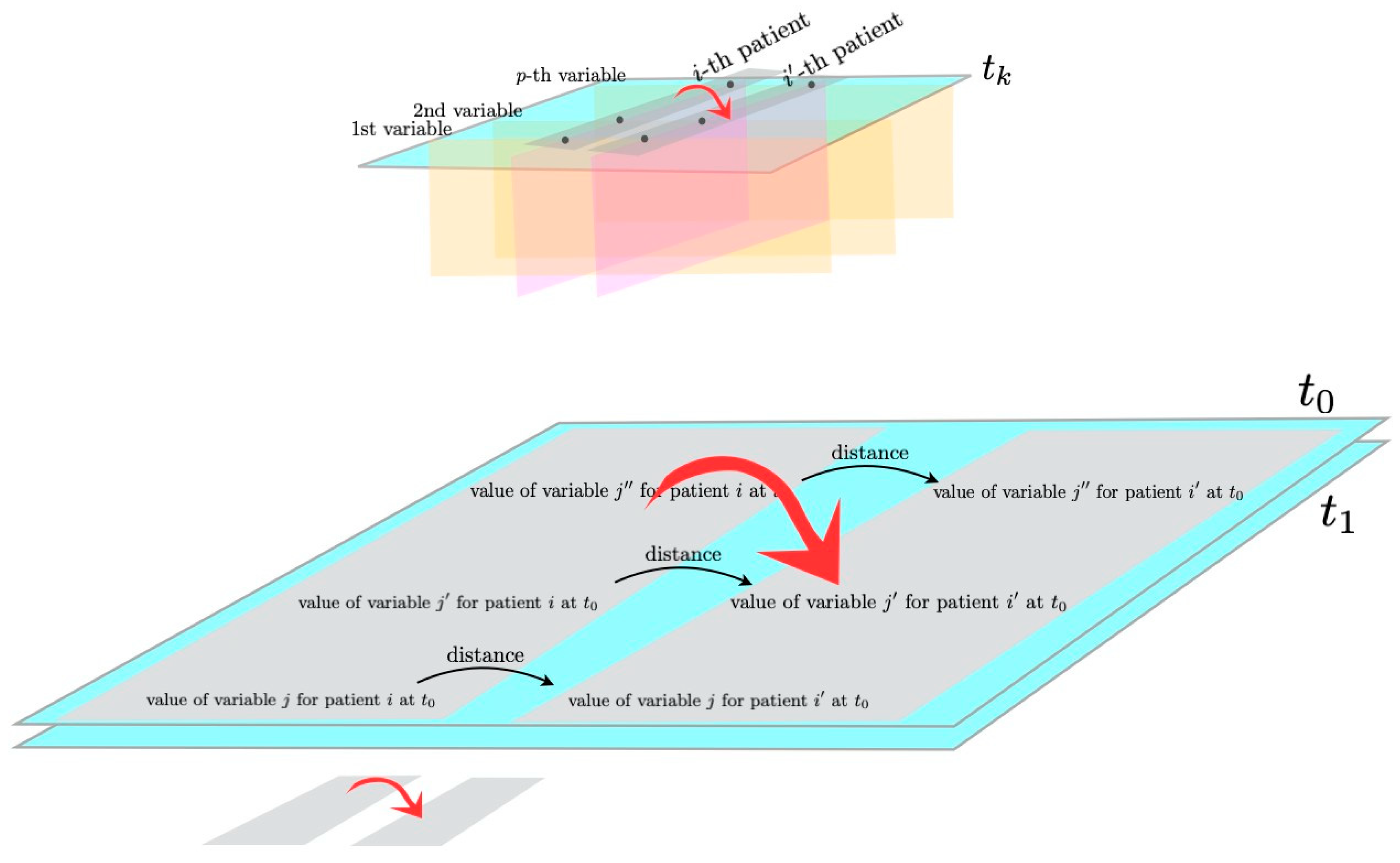
Figure 1. Representation of the Gower distance. The Gower distance between two patients at the same time point gives a scalar; that between all patients gives a dissimilarity matrix.
Stats 06 00048 g001
Figure 2. Representation of the dataset.
Stats 06 00048 g002
Figure 3. Comparison between values of the j-th variable for i , i patients at t 0 and t 1 .
Stats 06 00048 g003
Figure 4. Hierarchical dendrograms based on d ( t 0 ) (a), d ( t 1 ) (b), and d ( t 2 ) (c), respectively.
Stats 06 00048 g004
Figure 5. Dissimilarity matrices at each time point. The darker the color, the higher the similarity. Patients are arranged to highlight clusters. Identical patients are automatically shown in the secondary diagonal.
Stats 06 00048 g005
Figure 6. Comparison between two dissimilarity matrices.
Stats 06 00048 g006
Figure 7. Matrices indicating the variation of dissimilarity matrices from a time point to the consecutive one. The darker the color, the higher the similarity.
Stats 06 00048 g007
Table 1. Characteristics of patients at t 0 .
Continuous VariableMean (Standard Deviation)
body mass index (BMI)31.77 (5.56)
diastolic pressure79.29 (10.05)
glycated hemoglobin (HbA1c)7.34 (1.24)
mean ratio of albumine to serum creatinine (UACR)73.27 (259.67)
estimated glomerular filtration rate (eGFR)63.38 (15.81)
triglycerides182.1 (157.00)
Nominal VariableDistribution
serum potassium1 (1.3%), 2 (63.4%), 3 (35.3%)
mean arterial pressure2 (63%), 3 (37%)
blood glucose(40.4% yes)
C-reactive protein (CRP)(68.9% yes)
Table 2. Comparison of matrices and clusters.
Distance MatricesMean Values of DistancesInter-Cluster DistanceIntra-Cluster DistanceFrobenius Norm
d ( t 0 ) 0.23 (0.09)0.250.1158.25
d ( t 1 ) 0.24 (0.09)0.27 0.14 59.76
d ( t 2 ) 0.28 (0.10)0.31 0.18 71.16
Table 3. Descriptive statistics of clusters at each time point.
TimeClusterSizeWithin DistanceTriglyceridesBMIDiastolic PressureHbA1cMean UACReGFR
t 0 1210.10218.2433.8086.717.9041.2271.81
2620.09210.4831.3074.727.5546.4864.64
3330.09217.6332.0888.487.7067.8466.33
4390.18166.7933.5774.207.5089.0961.41
5480.09143.5630.3274.026.8750.9061.67
6320.16143.2530.6087.036.69164.2662.47
t 1 1660.10195.9130.9976.647.6255.0263.57
2420.17224.1732.5978.427.7580.8762.45
3990.17154.0830.7276.726.7246.4365.71
4280.14238.3234.0774.438.2234.7256.71
t 2 1650.23187.5731.3184.097.6274.8262.36
2720.20145.2231.5574.616.6361.2360.82
3570.13224.8431.4672.747.6127.9366.47
4410.17211.7131.1772.978.1895.1553.78
Table 4. Percentages of patients with controlled disease according to the given therapeutic treatments.
Drug before  t 1 % of Controlled Response at  t 1
Cluster 1Cluster 2Cluster 3Cluster 4
RASi60.0056.0062.9043.75
RASi + SGLT2i59.0975.0057.1466.67
RASi + MCRa50.0066.6745.450.00
RASi + GLP1a66.6766.6760.0066.67
Drug before t 2 % of Controlled Response at t 2
Cluster 1Cluster 2Cluster 3Cluster 4
RASi51.1147.5070.0056.52
RASi + SGLT2i63.6455.5672.7383.33
RASi + MCRa25.0066.670.0028.57
RASi + GLP1a100.0025.00100.00100.00
Table 5. Measures for D , the matrices of distances between distances.
Matrix/MeasureMeanFrobenius Norm of ( d ( t k ) d ( t k 1 ) ) Chebyshev Distance between d ( t k ) and d ( t k 1 )
D ( d ( t 0 ) , d ( t 1 ) ) 0.00726.2333.68
D ( d ( t 1 ) , d ( t 2 ) ) 0.04729.1541.50
Disclaimer/Publisher’s Note: The statements, opinions and data contained in all publications are solely those of the individual author(s) and contributor(s) and not of MDPI and/or the editor(s). MDPI and/or the editor(s) disclaim responsibility for any injury to people or property resulting from any ideas, methods, instructions or products referred to in the content.