Abstract
In surveys requiring cost efficiency, such as medical research, measuring the variable of interest (e.g., disease status) is expensive and/or time-consuming; however, we often have access to easily obtainable characteristics about sampling units. These characteristics are not typically employed in the data collection process. Judgment post-stratification (JPS) sampling enables us to supplement the random samples from the population of interest with these characteristics as ranking information. This paper develops methods based on the JPS samples for estimating categorical ordinal populations. We develop various estimators from the JPS data even for situations where the JPS suffers from empty strata. We also propose the JPS estimators using multiple ranking resources. Through extensive numerical studies, we evaluate the performance of the methods in estimating the population. Finally, the developed estimation methods are applied to bone mineral data to estimate the bone disorder status of women aged 50 and older.
1. Introduction
In survey sampling problems, we typically have various information (e.g., patient demographic characteristics) about the population. Despite their accessibility, these characteristics are not often used in data collection. We believe these characteristics can be used for ranking and post-stratification of the sampling units. The information, supplemented by the post-stratification, enables us to produce more representative samples from the population.
In bone disorder research, a patient’s bone mineral density (BMD) is measured through dual X-ray absorptiometry (DXA) imaging, a costly and time-consuming procedure. Although there are plenty of patients, BMD measurements are obtained from a small proportion of the population. In these situations, we randomly select sampling units from the population and form a comparison set for each examined patient. As BMD measurements are expensive, we use easily obtainable characteristics (such as age, weight, or BMD measurements from previous examinations) to rank the units (without measuring their BMD values) in their comparison sets. Through this sampling scheme, we can supplement the BMD observations with these extra judgment ranks. This extra information (obtained from rank-based stratification) enables us to better estimate patients’ bone disorder status.
Judgment post-stratification (JPS) sampling [1] and ranked set sampling (RSS) [2] are two cost-effective rank-based sampling designs. In RSS, the ranks of the measured units have to be pre-specified. Moreover, RSS data are collected after the ranking process. Unlike RSS, JPS enjoys post-stratification so that observations are obtained before ranking. The JPS scheme offers various advantages over its RSS counterpart. For example, if the ranking process is unreliable, one can simply ignore the ranks attached to the JPS samples. The JPS samples now form simple random samples (SRS) from the population. Thus, one can apply conventional statistical methods for analyzing the JPS data. Unlike JPS, RSS statistics are not identically distributed. Hence, ranks can not be separated from the RSS observations [3].
The following explains how one can obtain the judgment ranks and JPS data from the bone disorder example. Let be an initial SRS of size n representing the bone disorder status of patients . We shall supplement this initial SRS with judgment ranks and construct JPS data of size n. As measuring the bone status is costly, we only measured the bone status (i.e., x-value) of these n patients as our initial SRS. To assign a judgment rank to , we first take a sample of patients independently from the population and construct the comparison set for , say . Note that we do not measure the bone status of these patients. We then rank the patients in based on an easy-to-measure characteristic such as the age of patients. Let denote the judgment rank of in . Consequently, we consider as a JPS observation for patient , where is the bone disorder status of the patient and is the judgment rank assigned to using the age characteristic. Finally, we replicate the above procedure to obtain the JPS data for the bone disorder population.
In the JPS scheme, we supplement the initial SRS with judgment ranks using easy-to-measure characteristics. Because the judgment rank may differ from the true rank of in the i-th comparison set, the ranking is called imperfect in this case. Unlike imperfect JPS, when units are ranked based on the response variable X, is the true rank of . In this case, there is no ranking error, and the ranking is called perfect.
JPS sampling has been employed in many research studies and applications. The JPS method has been used to estimate the population mean [4,5]. The isotonic regression model was used by [6] to develop a class of isotonized estimators for the cumulative distribution function. A new class of estimators was proposed by [7] based on the multi-ranker JPS data. The properties of JPS samples were utilized by [8] for non-parametric inference of population quantiles. Dastbaravarde et al. [9] focused on the parametric inference from JPS samples. Omidvar et al. [10] estimated the finite mixture models with the JPS samples. The estimation problem of a binary population was studied by [11] using the properties of the JPS data. In the literature on the categorical ordinal variables, various researchers have studied the estimation of the ordinal population from RSS samples. Ordinal logistic regression was employed by [12] to estimate the ordinal population with RSS data. Hatefi and Alvandi [13] and Alvandi and Hatefi [14] recently used the RSS data with tie structures to estimate the ordinal population parameters. Despite the importance of the categorical ordinal variables and the challenges of the RSS [6], to the best of our knowledge, no research in the literature has explored the estimation problem of ordinal populations with JPS data. In this manuscript, we investigate the properties of JPS data to estimate categorical ordinal populations.
The contributions of this manuscript are as follows. To the best of our knowledge, for the first time in the literature on categorical ordinal data, we propose using the properties of JPS sampling to improve the estimation of population parameters. The JPS method, as a rank-based sampling method, enables us to incorporate easy-to-measure characteristics as ranking information into data collection. We then develop more efficient estimates than the commonly used estimates based on SRS data of the same size in estimating the categorical ordinal population proportions. Various estimates are available in the literature for population proportions using ranked set sampling (RSS). The RSS method results in independent order statistics from the population. Therefore, the ranks can not be separated from RSS observations if ranking information is unreliable. Unlike RSS, JPS augments the initial SRS data with artificial judgment ranks to improve the efficiency of the estimators. If the ranking information is unreliable, one can easily ignore the assigned ranks, and JPS observations can be treated as SRS data. We can then apply conventional methods in the literature to estimate the population proportions. It is known that ranking is not well-defined in multivariate cases. To this end, we propose multi-observer JPS estimators that can combine ranking information from multiple resources to improve the JPS proposal’s efficiency in estimating the population proportions. As another contribution, we develop the estimation methods using JPS data, which can handle the empty ranking strata in estimating the parameters. Last but not least, we develop isotonized JPS-based estimators to impose stochastic ordering constraints on the JPS statistics to deal with the sampling variability involved in JPS sampling from categorical ordinal populations.
This manuscript is organized as follows. In Section 2, we propose various estimation methods for ordinal population parameters. These methods include three estimators from JPS without empty strata and six JPS estimators with empty strata. In Section 3, the estimation problem is extended to JPS data from multiple rankers. In Section 4, through extensive simulation studies, we evaluate the performance of the estimators. The proposed methods are applied to analyze bone disorder in a population of older people in Section 5. Finally, we present a summary and concluding remarks in Section 6.
2. Estimation Methods
Let follow a multinomial distribution with Q ordinal categories; that is, with and . The Q-dimensional random variable with and represents one draw out of Q categories of the population where one and only one entry of the vector is one and the other entries are zero. The location of one represents the category of the observation (out of Q categories). As in the multinomial distribution, the number of observations from categories is used to estimate the population proportions; this Q-dimensional vector representation may not be the best representation of the multinomial distribution. Specifically, in this manuscript, we would like to incorporate ranking information into the estimation. For these reasons, let , with support , be the univariate representation of the ordinal population. Note that there is a one-to-one mapping between the above representations and X. Additionally, let denote the cumulative probabilities where , with and in all the estimation methods. Let represent a JPS sample of size n with judgment ranks . Because the H units in the comparison sets are independent and identically distributed in the population, the JPS observation can equally likely take any rank in the comparison set . Therefore, (the rank of ) in comparison set j follows discrete uniform distribution on [9]. In this section, we propose various estimation methods based on JPS data for population proportions.
2.1. Standard Non-Parametric Estimators
We consider the estimation of the ordinal population based on commonly-used simple random sample/sampling (SRS). Note that, when we ignore the ranks of JPS data, can be treated as an SRS of size n.
Let denote the number of SRS data obtained from categories ; that is, , where represents an indicator function that if , otherwise . Suppose and . The standard estimator of from the SRS is given by:
The population proportions are then estimated by for , where . We now focus on estimation of the parameters of the categorical ordinal population based on JPS data. Let represent the number of JPS data obtained from rank stratum h. Let be the probability that a JPS observation with rank h comes from category q. Hence,
where for any . Similarly, let be the probability that a JPS observation with rank h comes from categories . Hence,
Let denote the number of JPS data from the h-th rank stratum from categories ; that is, . We define and . Hence, the standard JPS estimator of is given by:
Using (2), the standard JPS estimator of is obtained by:
The population proportions under the standard JPS are then estimated by for , where .
2.2. Maximum Likelihood Estimator
We use the maximum likelihood (ML) method to estimate the ordinal population proportions based on JPS data. Let be an SRS of size H from an ordinal distribution with categories where . Let represent the h-th order statistic in a set of size H units. For , following [15], one can easily show that with
where
denotes the incomplete beta function for , with .
For the sake of consistency in notations, as before, let , with support , be the univariate representation of the population. Let with ranks denote a perfect JPS sample (i.e., ranking is done based on X values, and there is no ranking error) of size n from the population. Given , represents the -th order statistic in the set of H units. Thus, the conditional log-likelihood function of can be constructed as follows (where the proof can be found in Appendix A):
where as an incomplete beta function of is given by (4). Hence, the log-likelihood function is written as a function of on the left-hand side of (5). From (5), the ML estimator of from JPS data is given by:
where the constraint is implied by the fact that the multinomial population has Q categories, where Q is given and in the population. To meet this requirement, throughout the manuscript for all the estimation methods, including the ML method, we only focus on the samples with at least one observation from all categories in the initial SRS. To find the maximum of the log-likelihood function (5), we treated the as incomplete beta functions of . We then used the linear constraint optimization via the constrOptim command in R, subject to constraints and for , to estimate a legitimate multinomial distribution in the numerical optimizations. We used the estimates from the standard JPS method as the starting values. The stopping rule was built by the convergence tolerance and the maximum number of iterations of 1000. Note that we developed the ML estimators assuming that there is no ranking error in the JPS; however, ranking error is undeniable in real-life applications where ranking is carried out through auxiliary variables. Accordingly, we assess the performance of the estimators in the presence of ranking errors in both simulation and real data analysis.
2.3. Non-Parametric Estimation Procedures
We apply the isotonized strategy [16] to the standard estimator and develop new non-parametric estimation procedures for an ordinal population using JPS data in the presence and absence of empty strata.
2.3.1. JPS Data without Empty Strata
We first study the isotonized estimation [16] for the population proportions, assuming that no empty stratum is observed in the JPS data. The JPS method, as a rank-based sampling method, creates artificial ranking strata on the sample space. It is more likely that individuals with smaller ranks come from smaller categories of the population; that is:
The constraint (7) may be violated owing to the sampling variability in the JPS data. Ozturk [16] proposed an isotonized strategy to impose stochastic ordering constraints among the ranking strata in estimating the cumulative density function based on ranked set samples. The isotonized estimation method was generalized by [6,11] to analyze the JPS data with empty strata in estimating the population mean and binary proportion, respectively. Following [6,11,16], we construct the isotonized version of the estimates by minimizing the weighted least squared errors under the above constraint where denotes the size of the rank strata r.
When the JPS has no empty strata, the isotonized estimator of can be obtained by either the MinMax method,
or the MaxMin isotonized estimator,
where and . Therefore, for the JPS data without empty strata, an isotonized estimator of the cumulative probability is given by:
When there are no empty strata, and yield an identical result. Hence, one can obtain (10) using either or as . To compute , one can first use an isotonized strategy for via the Pool Adjacent Violator Algorithm (PAVA) and then take the average. From , one can find the isotonized estimator of the population proportion by for , where .
2.3.2. JPS Data with Empty Strata
Now, we investigate the estimation of an ordinal population from JPS with empty strata. We propose four isotonized estimation procedures that include the naive estimator: ignoring the empty strata, MinMax, MaxMin, and mixed estimators. When JPS contains empty strata, Equations (8) and (9) may not be the same. In the presence of empty strata, the pooled cells (i.e., ) used in (8) and (9) may still be empty. The idea of the index set was developed by [6] as to deal with the empty strata. The MinMax and MaxMin estimators in the presence of empty strata are given by
where and are given by (2).
When JPS data have empty strata, the first approach can be simply an estimator ignoring the empty strata. After dropping the empty strata, one can obtain the isotonized estimate of the proportions in a similar fashion as in Section 2.3.1. This estimator is also denoted by to emphasize that empty strata have been ignored in the isotonized strategy.
Using (11) and (12), we propose our next estimators for proportions from the JPS data with empty strata. The MinMax isotonized estimator is given by , where are estimated from (11). In a similar vein, we use (12) and propose the MaxMin estimator by . The empty strata in the JPS data may result in empty pooled strata (i.e., ) in the isotonized strategy. Hence, the MaxMin and MinMax estimators differ when an empty stratum occurs. To compute the MinMax and MaxMin isotonized estimators, one can first implement the PAVA algorithm over non-empty cells and obtain the corresponding stratum proportion estimates. Note that an empty stratum is located at the boundary if the empty stratum is surrounded by empty strata on both sides. If the empty stratum is not at the boundary, the MinMax imputes the value by the closest non-empty stratum estimate on its left, while the MaxMin uses the closest non-empty stratum estimate on the right for imputation. When we face an empty cell at the boundary, then both MinMax and MaxMin estimators use the closest available non-empty stratum to estimate the empty values. For more information, see [17].
An isotonized estimator was proposed by [11] for the binary proportion by simply averaging the MaxMin and MinMax estimators. Following this study, we combine the two estimators and propose a new estimator for an ordinal population from JPS with empty strata. This combined estimator is given by , where and are the MaxMin and the MinMax estimators. Finally, similar to Section 2.3.1, one can obtain the isotonized estimators of from their corresponding isotonized estimators from the cumulative probabilities.
3. Extension to Multiple Rankers
In many applications, the ordinal variable is accompanied by several easy-to-measure concomitant variables. In these cases, multiple ranking information sets are available for each sampling unit. Therefore, it is important to combine ranking information from multiple resources and use them in the estimation process. In this section, we develop three estimators from the JPS data with multiple rankers for the ordinal population. These estimators include standard estimator, its isotonized counterpart, and a logistic regression-based estimator.
3.1. Standard and Isotonized Multi-Ranker Estimators
Suppose that we have access to ranking information from K rankers. Let represent the JPS data of size n, where is the judgment rank of assigned by ranker k for . Following [17], we propose a standard estimation method based on multi-ranker JPS. Here, the ranking information is first averaged for each JPS observation and then used in the estimation process. The standard estimator for for is given by
with and , where the ranking ability denotes the sample correlation between X and ranker k, namely , for .
Although there are K ranks available for each JPS observation here, the constraint (7) may still be violated by the standard multi-ranker estimator. Following [6], one can obtain the isotonized estimator of the population proportions from the JPS with multiple rankers. Thus, the multi-ranker estimator of for with isotonic properties is given by
where is the isotonized version of with weights , where
where and .
3.2. OLR-Based Estimation
Another methodology involves using the ordinal logistic regression (OLR) model to estimate the proportions from JPS with multiple rankers. The OLR model is utilized to combine information from multiple rankers into the estimation process. Let be the initial SRS of size n, from which we shall obtain JPS data of size n. Additionally, let represent the vector of ranking variables corresponding to the initial SRS. Following [12], we fit an OLR model with common slopes on the cumulative probabilities . The OLR model is given by
where , with slope and as the intercepts of the model. In this approach, we first estimate the parameters of the OLR model using the initial SRS of size n. The trained OLR model is then used to carry out the ranking involved in the JPS sampling.
We form a set of H units , including the first unit of the JPS data (say, , with variable of interest ) and randomly selected units from the population (without measuring their variable of interest). Applying the trained OLR model to , we rank the units based on , where smaller values are assigned bigger ranks. This is because the larger the value of , the more likely it is that the unit should come from a smaller category. In other words, one can easily see that the is an increasing function of . That is, the greater is, the greater will be, and thus the lower will be. When a unit attains a smaller , it is more likely that the unit will come from the larger categories, since is greater. Thus, it is more reasonable that the unit receives a higher rank in the comparison set. For more detail, see [12].
Through this approach, we find the rank (say, ) of . Similarly, we compute the ranks of all JPS observations using the trained OLR model. Let , with ranks , denote the JPS from the OLR model. Thus, the OLR-based JPS estimator of is given by
where
Finally, similar to Section 2.3.1, the multi-ranker JPS estimators of can be derived from their corresponding estimators of the cumulative probabilities.
4. Simulation Studies
We investigate the performance of the proposed methods in the estimation of an ordinal population. Let the variable of interest follow an ordinal population with three categories, i.e., , where . Here, we generate the ranking variable Z such that X and Z have correlation . Given , we generate Z by , where is the mean for X, is the standard deviation for X, and is a standard normal random variable that is independent of X.
In the simulation studies, we set the correlation to better explore the effect of ranking errors on the estimators. We generated JPS data of size with set size . For estimation of multiple rankers, we independently generated two concomitant variables, and , given X, such that and . We considered three combinations of concomitant variables to generate JPS with multiple rankers. These combinations include two strong rankers , one strong ranker and one moderate ranker , and two moderate rankers . To evaluate the effect of population configuration, we set and , and was treated as the dependent parameter. Because there are two levels for set size H, two levels for n, six combinations for ranking ability, nine estimation methods, and 16 population configurations, the total number of combinations investigated in the simulation studies accounts for . Due to this extensive number of combinations and the fact that there are three unknown mixing parameters , following [13,14], we selected these population configurations to be able to compare the pattern of all the estimators in each figure for various combinations at the same time. We set and then consider all possible values that can take. The configuration enables us to compare the performance of the proposed methods in situations where a small proportion of observations can come from the last category. On the other side, we set the maximum value . If , due to , then there are only two cases for ; that is, . Consequently, two points in a panel will not allow us to compare the pattern of the estimators well. When , the maximum value we consider for is 0.8, which implies that has to be 0.1 (i.e., ). Note that leads to the cases where the reference group has to be empty (as ), which contradicts the assumption of the underlying population with three categories. Accordingly, when , we consider that ranges between (0.1,0.5). Additionally, when , we show ranging between (0.1,0.3).
To compare the performance of the estimators, following [12,13,14], we used the total efficiency of the JPS estimators relative to their SRS counterparts of the same size. The total relative efficiency (RE) of a JPS estimator is given by
When the RE is greater than one, we can conclude that the JPS estimator outperforms its SRS counterpart in the estimation of the ordinal population.
We carried out two separate simulations to investigate the performance of the estimators using JPS without empty strata and JPS with empty strata. In the first simulation, we only focused on the JPS data without empty strata. To do that, when the JPS sample was generated, we first checked to see if there was at least one observation from all rank strata. If not, we ignored the sample and kept independently sampling until we obtained a JPS sample without empty strata. We then applied the developed methods to the JPS sample to estimate the parameters based on the JPS data without empty strata. For JPS with empty strata, we carried out another simulation study. In this study, we generated a JPS sample and checked to see if there was at least one empty rank stratum. To do that, we first randomly selected the index of the empty strata. The proposed ranking design is accepted with probability 1/(number of empty strata) to favor the sample with the smaller number of empty strata. We then independently sampled from the population until we obtained a JPS sample compatible with the accepted ranking design. The obtained JPS sample has at least one empty stratum. We then used the JPS sample with at least one empty stratum to estimate the parameters of the population. For a fair evaluation, we simulated the JPS and SRS data 5000 times and computed the estimates of the population parameters for each combination .
Figure 1 and Figure 2 represent the performance of the estimators using the JPS without empty strata and the JPS with empty strata, respectively. It can be observed that the REs of the JPS estimators (both ML and non-parametric methods) are almost always greater than one.
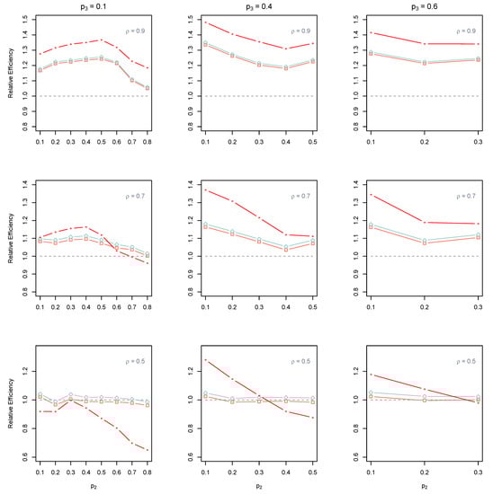
Figure 1.
The total REs of (□, red color), (◇, blue color), and (🟊, red color) from the JPS without empty strata compared to their SRS counterpart when . The dashed line represents that the RE equals to one.
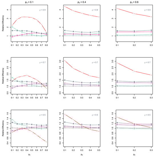
Figure 2.
The total REs of (□, red color), (◇, blue color), (▽, blue color), (△, red color), ( , blue color), and (🟊, red color) from the JPS with empty strata compared to their SRS counterpart when . The dashed line represents that the RE equals to one.
, blue color), and (🟊, red color) from the JPS with empty strata compared to their SRS counterpart when . The dashed line represents that the RE equals to one.
That is, one can more accurately estimate the ordinal population with JPS data than with SRS data of the same size. The effect of ranking ability is evident on the performance of the JPS estimators. When ranking ability is strong, the RE of the JPS estimators significantly grows as the set size H increases from 3 to 6. However, when the ranking ability is poor, the performance of the JPS estimators deteriorates, and the RE becomes almost one. In other words, when ranking is unreliable, the JPS estimators perform similar to their SRS counterparts in the estimation of the ordinal population (see Figure A1, Figure A2, Figure A3, Figure A4, Figure A5 and Figure A6). From Figure 2, we see that the RE of the ML estimators dramatically increases, and they considerably outperform all the non-parametric estimators so that the improvement of non-parametric JPS estimators is not noticeable at all. This dramatic superiority of the MLEs is compatible with the results of [11] (in estimation of binary proportion from JPS data). This dramatic increase is because of the dependence of the MLEs on the population configuration. When ranking is high and population parameters are away from zero, the MLEs are highly recommended. Otherwise, we observe that non-parametric estimators are more robust (than MLEs) to ranking errors and population configuration. We observe that more accurately estimates the population compared to other nonparametric methods when JPS has empty strata. This superiority of refers to the fact that it benefits from both and in the estimation.
Figure 3 and Figure 4 show the results of the estimations using the JPS data with multiple rankers. It can be seen that all estimators based on multi-ranker JPS outperform their SRS counterparts. The standard and the isotonized multi-ranker estimators perform better than OLR-based counterparts in the estimation of the parameters. The shortcoming of the OLR-based method may stem from the fact that the initial JPS sample was used in both training and prediction phases. Consequently, this reduces the ranking ability of the trained OLR model in the comparison sets in the case of new individuals (who were randomly selected from the population and were not used in the training phase). We see that the performance of multi-ranker estimators improves as the set size increases, and ranking ability is decent. Unlike the OLR-based estimator, the standard and isotonized multi-ranker estimators take full advantage of the high ranking ability and large set size so that their REs grow considerably in these situations. We also observe that the isotonized multi-ranker estimator almost always outperforms its standard counterpart.
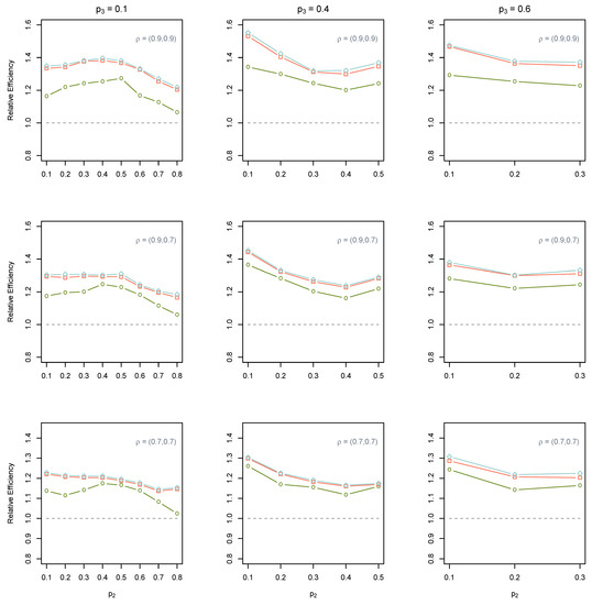
Figure 3.
The total REs of (○, green color), (□, red color), and (◇, blue color) from the JPS with multiple rankers compared to their SRS counterpart when . The dashed line represents that the RE equals to one.
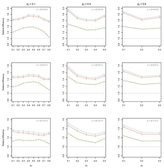
Figure 4.
The total REs of (○, green color), (□, red color), and (◇, blue color) from the JPS with multiple rankers compared to their SRS counterpart when . The dashed line represents that the RE equals to one.
5. Real Data Analysis
In this section, we applied the developed methods to an analysis of a bone disorder of women aged 50 and older. Here, the JPS samples were obtained from bone mineral density (BMD) data where measuring the variable of interest is expensive and time-consuming. Ranking in JPS data is carried out by using some characteristics associated with BMD measurement. Thus, ranking errors arise naturally in the JPS data.
Osteoporosis is a bone metabolic disorder that occurs when the density of the bone tissues deteriorates significantly. This deterioration leads to numerous major health problems, including skeletal fragility and osteoporotic fractures (such as of the hip). For example, more than 50% of patients suffering from osteoporotic hip fracture are not able to live independently, while around 28% of these patients will survive less than a year because of complications from the broken bones [18,19,20]. Prevalence of osteoporotic fractures increases as age increases. Hence, it is critical to monitor and diagnose the bone disorder status of the population, particularly for the aged population.
According to the expert panel of the World Health Organization, bone mineral density (BMD) is one of the most reliable predictors of a diagnosis of osteoporosis. BMD measurements are obtained via dual X-ray absorptiometry (DXA) imaging from various parts of the body, such as the femoral neck. Once the DXA images are acquired, they must be investigated by medical experts for manual segmentation and quantification of the final scores. The process of measuring the BMDs is costly and time-consuming. BMD measurements are usually reported as a T-score (a standardized score) showing the number standard deviations (SDs) from the BMD norm of the population. The BMD norm is calculated from the BMD measurements of young and healthy individuals between 20–30 years old. Using all the information from the population, the bone disorder status of a patient is diagnosed as osteoporosis when the T-score is more than 2.5 SDs below the BMD norm, i.e., . The bone status is determined as osteopenia when , and the status is considered normal when [21]. Thus, the bone disorder can be represented by an ordinal population with three categories.
In this study, we worked with BMD data from the National Health and Nutrition Examination Survey (NHANES III). The survey was conducted by the Centers for Disease Control and Prevention (CDC) on 33,999 Americans between the years 1988–1994. The survey consists of two examinations of BMD measurements from 234 women aged 50 and older. The examinations consist of the BMD measurements from different regions, including the femur neck (FNBMD), the trochanter region (TRBMD), and the inter-trochanter region (INBMD). In this analysis, we treated these 234 individuals as our underlying population. We also considered the FNBMD from the second examination as our variable of interest X, which follows an ordinal distribution with proportions with , and .
In this numerical study, to better assess the ranking error, we used FNBMD () and TRBMD () scores from the first bone examination for ranking purposes. The correlation levels of these two rankers with response variable X are and . Since these BMD scores are numerical, we rank the patients based on these scores. In JPS methods based on a single ranker, the higher the score value, the higher the rank the individual received in the comparison set. In multi-ranker standard JPS methods, as described in Section 3.1, we ranked the individuals based on the weighted average of the FNBMD and TRBMD scores. In the multi-ranker JPS method based on the OLR model, as described in Section 3.2, we first fitted an ordinal logit regression to the initial sample using and as the covariates of the regression. We estimated the OLR model parameters and then used the trained OLR model to assign the individual ranks within the comparison sets. Note that rank-based sampling designs, as cost-effective sampling techniques, have been widely used to analyze the BMD measurements. For instance, researchers in [10,13,14] analyzed the BMD population using the ranked set samples.
We selected JPS data of size with set size via sampling with replacement from the bone disorder population. For each combination , we replicated 5000 times the JPS data collection and computed the total REs (16) of the developed JPS estimators relative to their SRS counterpart of the same size. Similar to simulation studies, we used the initial SRS samples to train the OLR models. The results of the empirical study are illustrated in Table 1 and Table 2. It is apparent that the REs of all the JPS estimators are almost always greater than 1. Thus, JPS methods outperform their commonly used SRS counterpart in the estimation of the bone disorder population. From Table 1, when ranking ability is decent in the JPS (with and without empty strata), the REs of the JPS estimators improve. This improvement grows when set size increases from 3 to 6. In addition, the ML estimators always outperform the non-parametric estimators. This superiority is compatible with what we observed in simulation studies, namely that the RE of the ML estimators dramatically increases when ranking ability is high and population proportions are away from zero. Comparing the non-parametric estimators, the appears more promising in the estimation of the bone disorder population. From Table 2, the standard and isotonized multi-rankers perform better than their OLR-based counterpart. Finally, the isotonized multi-ranker estimator is recommended to practitioners for estimating the parameters of the bone disorder population.

Table 1.
The REs of the JPS estimators relative to their SRS counterparts when and .
Table 2.
The REs of JPS estimators using two rankers (FNBMD and TRBMD scores) relative to their SRS counterparts when and .
According to the complex data structure of the JPS statistics, there is no closed form for some of the proposed JPS estimators. For this reason, we ran another numerical study and numerically investigated the mean and standard error of the proposed JPS methods in estimating the proportions of the bone mineral population. As described earlier, we computed the JPS estimates of the proportions 3000 times and obtained the mean and standard errors of these 3000 estimates. Table A1, Table A2, Table A3 and Table A4 report the results of this numerical study. From Table A1 and Table A2, we can observe that the means of the JPS estimators, on average, are very close to the true values of the parameters; hence, one can conclude that the proposed JPS methods are almost unbiased in estimating the parameters of the bone mineral population. Comparing the standard errors from Table A3 and Table A4, we can see that the JPS methods appear, on average, more reliable than their SRS counterparts in estimating the proportions of the bone mineral population.
6. Summary and Concluding Remarks
In many applications, measuring the variable of interest is difficult; however, there may be easy-to-measure characteristics of the sampling units that can be effectively exploited for ranking and data collection process. Ranked set sampling and judgment post-stratification sampling are two cost-effective sampling schemes that use these characteristics as ranking information and enable us to obtain more representative sampling from the variable of interest.
Although refs. [12,14] have used the RSS data to estimate the ordinal proportions, the RSS data share various challenges in the data collection. For example, RSS data structure differs from the population structure, and ranking information cannot be separated from the RSS observations. Unlike RSS, JPS sampling results in a random sample of the population. If the ranking is unreliable, we can easily ignore the ranks. Thus, we can treat the JPS data as SRS data and apply conventional statistical methods to the JPS observations.
In this paper, to the best of our knowledge, we have studied for the first time the properties of the JPS samples for categorical ordinal variables. We developed various estimators using the JPS data. These estimators include three estimators based on the JPS without empty strata, six estimators from the JPS with empty strata, and three JPS estimators from multiple rankers. Through simulation studies, we investigated the effect of ranking error, set size, and population configuration on performance of the estimators. The developed estimators were then applied to an empirical example for analysis of bone disorder status of the aged population. From numerical investigation, we find that, when practitioners have access to a decent ranker, ML estimators are recommended for the estimation of the ordinal population. Otherwise, we recommend isotonized non-parametric estimators such as , which are more robust to ranking ability and population configuration.
As this manuscript is the first research to propose the properties of the JPS sampling in estimating the categorical ordinal population, our focus here is to develop these JPS-based estimation methods and show the superiority of the estimators relative to their counterparts based on commonly used SRS data. According to the complex data structure of the JPS statistics and the fact that there is no closed form for some of the proposed estimators, it may be insightful to study, in separate research, the finite sample properties of the developed JPS estimation methods, including bias, variance, and asymptotic behavior of the estimators.
Author Contributions
A.A. and A.H. conceptualized the research; A.H. developed the methodological parts; A.A. implemented the numerical studies; A.H. wrote the manuscript; A.H. guided the research. All authors have read and agreed to the submitted version of the manuscript.
Funding
The research of A.H. was supported by the Natural Sciences and Engineering Research Council of Canada (NSERC).
Institutional Review Board Statement
Not applicable.
Informed Consent Statement
Not applicable.
Data Availability Statement
The bone mineral data are publicly available on the website of the National Health and Nutrition Examination Survey at https://www.cdc.gov/nchs/nhanes/index.htm, (accessed on 1 August 2021).
Acknowledgments
Armin Hatefi acknowledges the research support of the Natural Sciences and Engineering Research Council of Canada (NSERC).
Conflicts of Interest
The authors declare no conflict of interest.
Appendix A
The following shows how the likelihood function, given the ranks in Equation (5), is constructed. Note that:
- (a)
- are iid random variables from a multinomial distribution with Q ordinal categories; that is, , and, for the sake consistency in notations, let denote their univariate representations.
- (b)
- Let , for . In perfect JPS, is the h-th order statistic in the i-th comparison set of size H.
- (c)
- are independent order statistics, since they come from independent comparison sets. Additionally, let denote their corresponding vector representations.
- (d)
- where
From (c) and (d), the likelihood function, given the ranks, is given by
Consequently, the log-likelihood function (i.e., Equation (5) in the manuscript) is constructed as:
Table A1.
The means of the JPS methods using a single ranker in estimating the bone mineral population proportions when and .
Table A1.
The means of the JPS methods using a single ranker in estimating the bone mineral population proportions when and .
| Ranker | n | H | p | With at Least One Empty Stratum | Without Empty Strata | |||||||
|---|---|---|---|---|---|---|---|---|---|---|---|---|
| FNBMD | 30 | 3 | 0.25 | 0.25 | 0.25 | 0.26 | 0.2 | 0.23 | 0.25 | 0.25 | 0.25 | |
| 0.66 | 0.66 | 0.66 | 0.66 | 0.69 | 0.68 | 0.66 | 0.66 | 0.66 | ||||
| 0.1 | 0.1 | 0.1 | 0.08 | 0.1 | 0.09 | 0.1 | 0.1 | 0.1 | ||||
| 6 | 0.25 | 0.25 | 0.25 | 0.26 | 0.23 | 0.24 | 0.25 | 0.25 | 0.25 | |||
| 0.66 | 0.66 | 0.66 | 0.65 | 0.67 | 0.66 | 0.66 | 0.66 | 0.66 | ||||
| 0.09 | 0.09 | 0.09 | 0.09 | 0.1 | 0.09 | 0.09 | 0.09 | 0.09 | ||||
| 60 | 3 | 0.25 | 0.25 | 0.25 | 0.26 | 0.2 | 0.23 | 0.25 | 0.25 | 0.25 | ||
| 0.66 | 0.66 | 0.66 | 0.67 | 0.7 | 0.69 | 0.66 | 0.66 | 0.66 | ||||
| 0.09 | 0.09 | 0.09 | 0.07 | 0.09 | 0.08 | 0.09 | 0.09 | 0.09 | ||||
| 6 | 0.25 | 0.25 | 0.25 | 0.26 | 0.23 | 0.24 | 0.25 | 0.25 | 0.25 | |||
| 0.67 | 0.67 | 0.67 | 0.66 | 0.68 | 0.67 | 0.67 | 0.67 | 0.67 | ||||
| 0.09 | 0.09 | 0.09 | 0.08 | 0.09 | 0.08 | 0.09 | 0.09 | 0.09 | ||||
| TRBMD | 30 | 3 | 0.25 | 0.25 | 0.25 | 0.26 | 0.21 | 0.24 | 0.25 | 0.25 | 0.25 | |
| 0.66 | 0.66 | 0.66 | 0.66 | 0.69 | 0.67 | 0.66 | 0.66 | 0.66 | ||||
| 0.09 | 0.09 | 0.09 | 0.08 | 0.1 | 0.09 | 0.09 | 0.09 | 0.09 | ||||
| 6 | 0.25 | 0.25 | 0.25 | 0.26 | 0.23 | 0.24 | 0.25 | 0.25 | 0.25 | |||
| 0.66 | 0.66 | 0.66 | 0.65 | 0.67 | 0.66 | 0.66 | 0.66 | 0.66 | ||||
| 0.09 | 0.09 | 0.09 | 0.09 | 0.1 | 0.09 | 0.09 | 0.09 | 0.09 | ||||
| 60 | 3 | 0.25 | 0.25 | 0.25 | 0.26 | 0.21 | 0.24 | 0.25 | 0.25 | 0.25 | ||
| 0.66 | 0.66 | 0.66 | 0.67 | 0.69 | 0.68 | 0.66 | 0.66 | 0.66 | ||||
| 0.09 | 0.09 | 0.09 | 0.07 | 0.09 | 0.08 | 0.09 | 0.09 | 0.09 | ||||
| 6 | 0.25 | 0.25 | 0.25 | 0.26 | 0.23 | 0.25 | 0.25 | 0.25 | 0.25 | |||
| 0.67 | 0.67 | 0.67 | 0.66 | 0.68 | 0.67 | 0.67 | 0.67 | 0.67 | ||||
| 0.09 | 0.09 | 0.09 | 0.08 | 0.09 | 0.08 | 0.09 | 0.09 | 0.09 | ||||

Figure A1.
The total REs of (□, red color), (◇, blue color), and (🟊, red color) from the JPS without empty strata compared to their SRS counterparts when . The dashed line represents that the RE equals to one.
Figure A1.
The total REs of (□, red color), (◇, blue color), and (🟊, red color) from the JPS without empty strata compared to their SRS counterparts when . The dashed line represents that the RE equals to one.


Figure A2.
The total REs of (□, red color), (◇, blue color), and (🟊, red color) from the JPS without empty strata compared to their SRS counterparts when . The dashed line represents that the RE equals to one.
Figure A2.
The total REs of (□, red color), (◇, blue color), and (🟊, red color) from the JPS without empty strata compared to their SRS counterparts when . The dashed line represents that the RE equals to one.


Figure A3.
The total REs of (□, red color), (◇, blue color), and (🟊, red color) from the JPS without empty strata compared to their SRS counterparts when . The dashed line represents that the RE equals to one.
Figure A3.
The total REs of (□, red color), (◇, blue color), and (🟊, red color) from the JPS without empty strata compared to their SRS counterparts when . The dashed line represents that the RE equals to one.


Figure A4.
The total REs of (□, red color), (◇, blue color), (▽, blue color), (△, red color), (, blue color), and (🟊, red color) from the JPS with empty strata compared to their SRS counterparts when . The dashed line represents that the RE equals to one.
, blue color), and (🟊, red color) from the JPS with empty strata compared to their SRS counterparts when . The dashed line represents that the RE equals to one.

Figure A5.
The total REs of (□, red color), (◇, blue color), (▽, blue color), (△, red color), (, blue color), and (🟊, red color) from the JPS with empty strata compared to their SRS counterparts when . The dashed line represents that the RE equals to one.
, blue color), and (🟊, red color) from the JPS with empty strata compared to their SRS counterparts when . The dashed line represents that the RE equals to one.

Figure A6.
The total REs of (□, red color), (◇, blue color), (▽, blue color), (△, red color), (, blue color), and (🟊, red color) from the JPS with empty strata compared to their SRS counterparts when . The dashed line represents that the RE equals to one.
, blue color), and (🟊, red color) from the JPS with empty strata compared to their SRS counterparts when . The dashed line represents that the RE equals to one.

Figure A7.
The total REs of (○, green color), (□, red color), and (◇, blue color) from the JPS with multiple rankers compared to their SRS counterparts when . The dashed line represents that the RE equals to one.
Figure A7.
The total REs of (○, green color), (□, red color), and (◇, blue color) from the JPS with multiple rankers compared to their SRS counterparts when . The dashed line represents that the RE equals to one.


Figure A8.
The total REs of (○, green color), (□, red color), and (◇, blue color) from the JPS with multiple rankers compared to their SRS counterparts when . The dashed line represents that the RE equals to one.
Figure A8.
The total REs of (○, green color), (□, red color), and (◇, blue color) from the JPS with multiple rankers compared to their SRS counterparts when . The dashed line represents that the RE equals to one.

Table A2.
The standard errors of the JPS methods using a single ranker in estimating the bone mineral population proportions when and .
Table A2.
The standard errors of the JPS methods using a single ranker in estimating the bone mineral population proportions when and .
| Ranker | n | H | p | With at Least One Empty Stratum | Without Empty Strata | |||||||
|---|---|---|---|---|---|---|---|---|---|---|---|---|
| FNBMD | 30 | 3 | 0.13 | 0.13 | 0.13 | 0.13 | 0.09 | 0.1 | 0.13 | 0.13 | 0.13 | |
| 0.12 | 0.11 | 0.11 | 0.13 | 0.1 | 0.11 | 0.12 | 0.11 | 0.11 | ||||
| 0.06 | 0.06 | 0.06 | 0.04 | 0.07 | 0.05 | 0.06 | 0.06 | 0.06 | ||||
| 6 | 0.1 | 0.09 | 0.08 | 0.08 | 0.07 | 0.07 | 0.1 | 0.09 | 0.08 | |||
| 0.1 | 0.09 | 0.09 | 0.09 | 0.09 | 0.08 | 0.1 | 0.09 | 0.09 | ||||
| 0.05 | 0.05 | 0.05 | 0.04 | 0.05 | 0.04 | 0.05 | 0.05 | 0.05 | ||||
| 60 | 3 | 0.12 | 0.12 | 0.12 | 0.12 | 0.08 | 0.09 | 0.12 | 0.12 | 0.12 | ||
| 0.1 | 0.1 | 0.1 | 0.12 | 0.08 | 0.1 | 0.1 | 0.1 | 0.1 | ||||
| 0.06 | 0.06 | 0.06 | 0.04 | 0.06 | 0.05 | 0.06 | 0.06 | 0.06 | ||||
| 6 | 0.08 | 0.07 | 0.07 | 0.06 | 0.05 | 0.05 | 0.08 | 0.07 | 0.07 | |||
| 0.08 | 0.07 | 0.07 | 0.07 | 0.07 | 0.06 | 0.08 | 0.07 | 0.07 | ||||
| 0.04 | 0.04 | 0.04 | 0.03 | 0.04 | 0.04 | 0.04 | 0.04 | 0.04 | ||||
| TRBMD | 30 | 3 | 0.12 | 0.12 | 0.12 | 0.12 | 0.09 | 0.1 | 0.12 | 0.12 | 0.12 | |
| 0.11 | 0.11 | 0.11 | 0.11 | 0.1 | 0.1 | 0.11 | 0.11 | 0.11 | ||||
| 0.06 | 0.06 | 0.06 | 0.04 | 0.06 | 0.05 | 0.06 | 0.06 | 0.06 | ||||
| 6 | 0.09 | 0.08 | 0.08 | 0.08 | 0.07 | 0.07 | 0.09 | 0.08 | 0.08 | |||
| 0.09 | 0.08 | 0.08 | 0.08 | 0.07 | 0.07 | 0.09 | 0.09 | 0.09 | ||||
| 0.05 | 0.05 | 0.05 | 0.04 | 0.05 | 0.05 | 0.05 | 0.05 | 0.05 | ||||
| 60 | 3 | 0.11 | 0.11 | 0.11 | 0.1 | 0.08 | 0.09 | 0.11 | 0.11 | 0.11 | ||
| 0.09 | 0.09 | 0.09 | 0.1 | 0.07 | 0.08 | 0.09 | 0.09 | 0.09 | ||||
| 0.05 | 0.05 | 0.05 | 0.04 | 0.06 | 0.04 | 0.05 | 0.05 | 0.05 | ||||
| 6 | 0.07 | 0.07 | 0.07 | 0.06 | 0.05 | 0.05 | 0.07 | 0.07 | 0.07 | |||
| 0.07 | 0.07 | 0.07 | 0.07 | 0.06 | 0.06 | 0.07 | 0.07 | 0.07 | ||||
| 0.04 | 0.04 | 0.04 | 0.03 | 0.04 | 0.04 | 0.04 | 0.04 | 0.04 | ||||
Table A3.
The means of JPS methods using two rankers (FNBMD and TRBMD scores) in estimating the bone mineral population proportions when and .
Table A3.
The means of JPS methods using two rankers (FNBMD and TRBMD scores) in estimating the bone mineral population proportions when and .
| n | H | p | |||
|---|---|---|---|---|---|
| 30 | 3 | 0.25 | 0.25 | 0.25 | |
| 0.66 | 0.66 | 0.66 | |||
| 0.09 | 0.09 | 0.09 | |||
| 6 | 0.25 | 0.25 | 0.25 | ||
| 0.66 | 0.66 | 0.66 | |||
| 0.09 | 0.09 | 0.09 | |||
| 60 | 3 | 0.25 | 0.25 | 0.25 | |
| 0.67 | 0.67 | 0.67 | |||
| 0.09 | 0.09 | 0.09 | |||
| 6 | 0.25 | 0.25 | 0.25 | ||
| 0.67 | 0.67 | 0.67 | |||
| 0.09 | 0.09 | 0.09 |
Table A4.
The standard errors of the JPS methods using two rankers (FNBMD and TRBMD scores) in estimating the bone mineral population proportions when and .
Table A4.
The standard errors of the JPS methods using two rankers (FNBMD and TRBMD scores) in estimating the bone mineral population proportions when and .
| n | H | p | |||
|---|---|---|---|---|---|
| 30 | 3 | 0.07 | 0.06 | 0.06 | |
| 0.08 | 0.08 | 0.08 | |||
| 0.04 | 0.04 | 0.04 | |||
| 6 | 0.07 | 0.06 | 0.06 | ||
| 0.08 | 0.07 | 0.07 | |||
| 0.04 | 0.04 | 0.04 | |||
| 60 | 3 | 0.05 | 0.04 | 0.04 | |
| 0.05 | 0.05 | 0.05 | |||
| 0.03 | 0.03 | 0.03 | |||
| 6 | 0.05 | 0.04 | 0.04 | ||
| 0.05 | 0.04 | 0.04 | |||
| 0.03 | 0.03 | 0.03 |
References
- MacEachern, S.N.; Stasny, E.A.; Wolfe, D.A. Judgement post-stratification with imprecise rankings. Biometrics 2004, 60, 207–215. [Google Scholar] [CrossRef] [PubMed]
- McIntyre, G.A. A method for unbiased selective sampling, using ranked sets. Aust. J. Agric. Res. 1952, 30, 385–390. [Google Scholar] [CrossRef]
- Chen, Z.; Bai, Z.; Sinha, B. Ranked Set Sampling: Theory and Applications; Springer: New York, NY, USA, 2013. [Google Scholar]
- Wang, X.; Stokes, L.; Lim, J.; Chen, M. Concomitants of multivariate order statistics with application to judgment post-stratification. J. Am. Stat. Assoc. 2006, 101, 1693–1704. [Google Scholar] [CrossRef]
- Frey, J.; Feeman, T.G. An improved mean estimator for judgment post-stratification. Comput. Stat. Data Anal. 2012, 56, 418–426. [Google Scholar] [CrossRef]
- Wang, X.; Lim, J.; Stokes, L. A nonparametric mean estimator for judgment post-stratified data. Biometrics 2008, 64, 355–363. [Google Scholar] [CrossRef]
- Ozturk, O. Combining ranking information in judgment post stratified and ranked set sampling designs. Environ. Ecol. Stat. 2012, 19, 73–93. [Google Scholar] [CrossRef]
- Ozturk, O. Statistical inference for population quantiles and variance in judgment post-stratified samples. Comput. Stat. Data Anal. 2014, 77, 188–205. [Google Scholar] [CrossRef]
- Dastbaravarde, A.; Arghami, N.R.; Sarmad, M. Some theoretical results concerning nonparametric estimation by using a judgment poststratification sample. Commun. Stat.—Theory Methods 2016, 45, 2181–2203. [Google Scholar] [CrossRef][Green Version]
- Omidvar, S.; Jafari Jozani, M.; Nematollahi, N. Judgment post-stratification in finite mixture modeling: An example in estimating the prevalence of osteoporosis. Stat. Med. 2018, 37, 4823–4836. [Google Scholar] [CrossRef] [PubMed]
- Zamanzade, E.; Wang, X. Estimation of population proportion for judgment post-stratification. Comput. Stat. Data Anal. 2017, 112, 257–269. [Google Scholar] [CrossRef]
- Chen, H.; Stasny, E.A.; Wolfe, D.A. Ranked set sampling for ordered categorical variables. Can. J. Stat. 2008, 36, 179–191. [Google Scholar] [CrossRef]
- Hatefi, A.; Alvandi, A. Efficient estimators with categorical ranked set samples: Estimation procedures for osteoporosis. J. Appl. Stat. 2022, 49, 803–818. [Google Scholar] [CrossRef] [PubMed]
- Alvandi, A.; Hatefi, A. Estimation of ordinal population with multi-observer ranked set samples using ties information. Stat. Methods Med. Res. 2021, 30, 1960–1975. [Google Scholar] [CrossRef] [PubMed]
- David, H.A.; Nagaraja, H.N. Order Statistics, 3rd ed.; John Wiley & Sons: Hoboken, NJ, USA, 2004. [Google Scholar]
- Ozturk, O. Statistical inference under a stochastic ordering constraint in ranked set sampling. J. Nonparametr. Stat. 2007, 19, 131–144. [Google Scholar] [CrossRef]
- Wang, X.; Wang, K.; Lim, J. Isotonized cdf estimation from judgment poststratification data with empty strata. Biometrics 2012, 68, 194–202. [Google Scholar] [CrossRef] [PubMed]
- Neuburger, J.; Currie, C.; Wakeman, R.; Tsang, C.; Plant, F.; De Stavola, B.; Cromwell, D.A.; van der Meulen, J. The impact of a national clinician-led audit initiative on care and mortality after hip fracture in england: An external evaluation using time trends in non-audit data. Med. Care 2015, 53, 686–691. [Google Scholar] [CrossRef] [PubMed]
- Bliuc, D.; Nguyen, N.D.; Milch, V.E.; Nguyen, T.V.; Eisman, J.A.; Center, J.R. Mortality risk associated with low-trauma osteoporotic fracture and subsequent fracture in men and women. J. Am. Med. Assoc. 2009, 301, 513–521. [Google Scholar] [CrossRef] [PubMed]
- Harvey, N.; Dennison, E.; Cooper, C. Osteoporosis: Impact on health and economics. Nat. Rev. Rheumatol. 2010, 6, 99–105. [Google Scholar] [CrossRef] [PubMed]
- Kanis, J.A. Diagnosis of osteoporosis and assessment of fracture risk. Lancet 2002, 359, 1929–1936. [Google Scholar] [CrossRef] [PubMed]


Disclaimer/Publisher’s Note: The statements, opinions and data contained in all publications are solely those of the individual author(s) and contributor(s) and not of MDPI and/or the editor(s). MDPI and/or the editor(s) disclaim responsibility for any injury to people or property resulting from any ideas, methods, instructions or products referred to in the content. |
© 2023 by the authors. Licensee MDPI, Basel, Switzerland. This article is an open access article distributed under the terms and conditions of the Creative Commons Attribution (CC BY) license (https://creativecommons.org/licenses/by/4.0/).