Abstract
COVID-19 spread dramatically across the world in the beginning of 2020. This paper presents a novel alert system that will detect abrupt changes in the COVID-19 or other pandemic incidence rate through the estimated time-varying reproduction number (Rt). We applied the system to detect abrupt changes in the COVID-19 pandemic incidence rates in thirteen world regions with eight in the US and five across the world. Subsequently, we also evaluated the system with the 2009 H1N1 pandemic in Hong Kong. Our system performs well in detecting both the abrupt increases and decreases. Users of the system can obtain accurate information on the changing trend of the pandemic to avoid being misled by low incidence numbers. The world may face other threatening pandemics in the future; therefore, it is crucial to have a reliable alert system to detect impending abrupt changes in the daily incidence rates. An added benefit of the system is its ability to detect the emergence of viral mutations, as different virus strains are likely to have different infection rates.
1. Introduction
In December 2019, four viral pneumonias were reported in Wuhan, China [1]. On 3 January 2020, 44 patients with pneumonia of unknown etiology were reported to the World Health Organization (WHO) by China. In a short period, COVID-19, named by the WHO on 11 February 2020, spread dramatically around the world. On 11 March 2020, the WHO declared the COVID-19 outbreak a global pandemic [2]. According to the WHO COVID-19 dashboard [3], there have been 527 million confirmed cases including 6 million deaths as of 31 May 2022. At the same time, many studies about this pandemic were conducted that focused on the spectrum of the clinical presentation [4], clinical characteristics [5] and incidence patterns [6].
During the period of a pandemic, one of the most important datum available is the incidence number. The curve of the daily infected cases indicates not only the size of the pandemic but also the transmissibility [7]. The incidence number can provide an intuition about the state of the pandemic; usually, a higher daily incidence number indicates a more severe pandemic. However, sometimes the incidence number can be misleading. For example, a low incidence number with a high increasing momentum foretells an impending disaster, namely, a dramatic increase in cases.
Another critical epidemiological measure is the basic reproduction number or the time-varying reproduction number , which represents the average cases infected by a single infected individual [8,9]. The infection is in control when and spreading if . There are several methods available to estimate the reproduction numbers and , including the exponential growth model [10], SIR method [11], Frequentists’ maximum likelihood method [12] and Bayesian framework [13]. The exponential growth model assumes that the daily cases can be viewed as an exponential growth during the early phase of the outbreak. In this model, the reproduction number can be denoted by the exponential growth rate. The SIR model is a traditional model that estimates the reproduction number by tracking the number of susceptible subjects, infected cases and recovered cases during a pandemic with the ordinary differential equations. The maximum likelihood method and the Bayesian method are classical statistical methods for estimating the reproduction numbers.
Many research works have focused on estimating the reproduction number of COVID-19 [14,15,16]; however, few have applied the reproduction number towards predicting the daily incidence [17] or detecting an abrupt increase in the daily cases. One staged alert system [18] based on the traditional SEIR model and seven-day average hospital admissions was designed to help ensure adequate ICU capacity by minimizing the duration of mitigation measures. As the hospitalization counts may present an unreliable signal, this model has met some practical challenges in applications. Another alert/detection system using the recurrent neural network [19] could identify the next wave of daily cases. However, since the neural network requires a large amount of training data, this system performed poorly in several regions with modest data size. Furthermore, this system could not alert people on the first wave of cases because there was no training data before the first wave.
To fill the void, in this study, we build a prediction system of the incidence numbers based on the estimated daily time-varying reproduction number that can alert people on impending abrupt changes in the pandemic incidence rate. The maximum likelihood estimation of is obtained with the MCMC method based on the serial interval distribution and previous daily incidence numbers. An alert will be given based on whether the estimated reproduction number is greater than 1. Meanwhile, the distribution of the new incidence number is simulated based on the estimated using the MCMC method. According to the comparison of the reported daily incidence number and the simulated distribution, abrupt increase and decrease trends will be captured by our system with the corresponding alert and/or notation given. We apply this new system to detect abrupt changes in the incidence rates for the 2009 H1N1 pandemic in Hongkong as well as the COVID-19 pandemic in different regions of the US and the world. The results show that our system can estimate the pandemic development and detect abrupt changes successfully.
2. Data and Methods
2.1. Data
In this study, the COVID-19 and H1N1 daily confirmed data from different regions were collected from the following resources:
- 1.
- The COVID-19 daily confirmed cases data of different regions:
- a.
- The states and cities in the United States [February 2020 to May 2022] were gathered from the COVID Data Tracker [20,21].
- b.
- England [February 2020 to May 2022] was gathered from the UK Government [22].
- c.
- New South Wales, Quebec, Hong Kong and Singapore [February 2020 to May 2022] were gathered from the Center for Systems Science and Engineering (CSSE) at Johns Hopkins University [23,24].
- 2.
- The H1N1 daily confirmed cases data in Hong Kong [April 2009 to February 2010] was gathered from On Kwok et al. 2015 [25].
To avoid the effect of unusual data due to the record style among the different regions and the weekly pattern of incidence number, we adopted the seven-day rolling average data to replace the raw daily data. In the following analysis and results, the daily incidence number refers to the rolling average of the incidence number, which is calculated with the following equation:
2.2. Method
The basic process of our prediction and detection system can be divided into three parts as shown in Figure 1:
- a.
- Estimation of the time-varied reproduction number (): Utilize the serial interval distribution and historical daily incidence numbers to calculate the maximum likelihood estimation of the daily time-varied reproduction number () with the Markov Chain Monte Carlo (MCMC) method. Alert 1 will be generated when the value of is greater than 1. Alert 1 indicates that the infectious disease is in an outbreak period.
- b.
- Simulation of the distribution of the incidence number of the following day (): With the historical daily incidence numbers (It-p…, It) and the estimated , the distribution of is simulated with the MCMC method. Comparing the reported value of the following day’s incidence number It+1 with the simulated distribution, Alert 2 or Note will be given if the reported value falls outside the forecast interval. Alert 2 identifies the potential abrupt increase in the incidence number, while Note indicates the potential abrupt decrease.
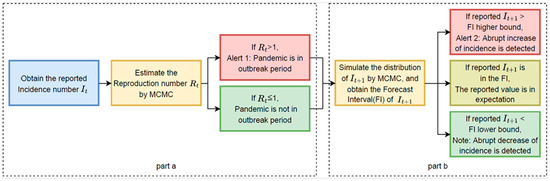
Figure 1.
Flow Chart. Flow chart of the proposed alert system forecasting abrupt changes in the pandemic incidence rate consisting of two stages/parts.
Figure 1.
Flow Chart. Flow chart of the proposed alert system forecasting abrupt changes in the pandemic incidence rate consisting of two stages/parts.
Based on the historical incidence number, , our detection and prediction system estimates the time-varying reproduction number and simulates the distribution of a new incidence number . Alert 1 will be generated on day t if the estimated value of Rt is greater than 1, and Alert 2 will be given on day t + 1 if the incidence number at day t + 1, is higher than the higher bound of the simulated forecast interval. Furthermore, Note will be given when is lower than the lower bound of the simulated forecast interval. Alert 1 is an alert to indicate that the infectious disease is in an outbreak period, while Alert 2 and Note identify the potential abrupt increase or decrease in the incidence number. In our application, to avoid redundancy, Alert 2 will not be given again if Alert 2 has already been given during the previous five days, and Note will not be given again if Note has already been given during the previous five days.
2.2.1. Estimation of and Generation of Alert 1
In this study, we adopted an intuitive method [13] to estimate based on its definition. The instantaneous reproduction number [26] can be estimated with the ratio of the new incidence number at day t (It) to the total infectiousness of infected individuals at time t, which can be noted with the weighted average of the infection incidence number up to time t − 1, . Here, represents the expectation of the number of secondary cases infected by each infected person if the conditions remained the same as time t [13].
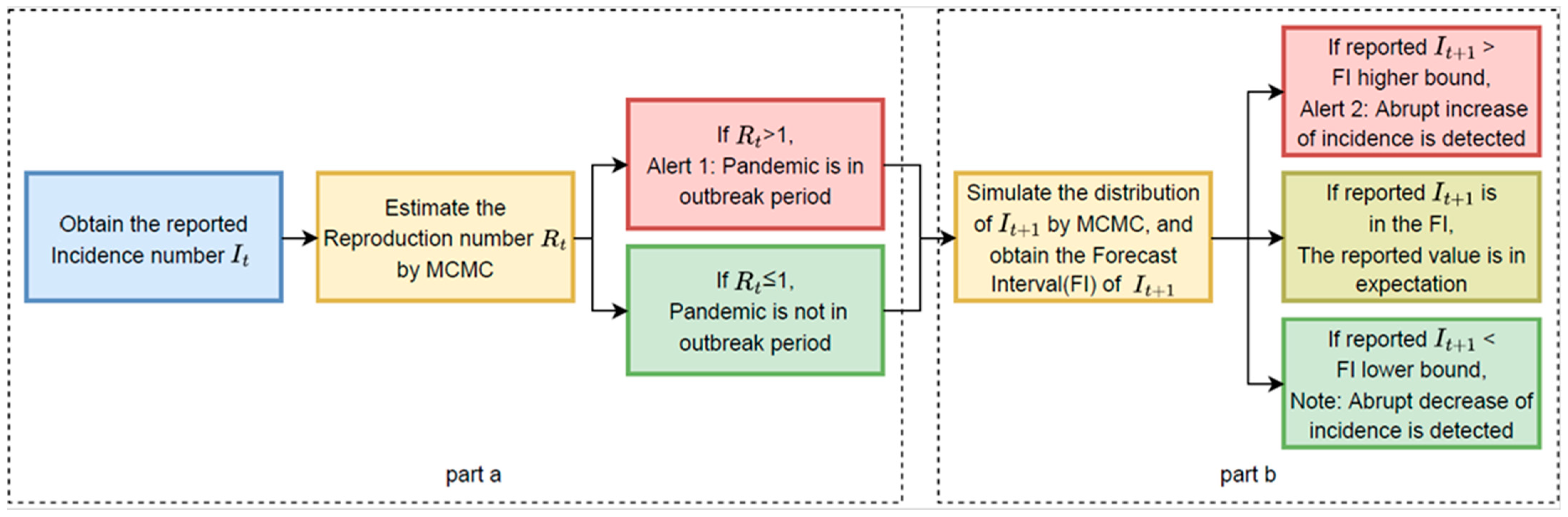
The serial interval distribution, which is the time between successive cases in a chain of transmission [27], is usually used as the weight [13]. The distribution will be changed for different diseases or different variants of the same disease.
We incorporate different variants of the SARS-CoV-2 coronavirus by using the log normal distributions with different means and standard deviations as the serial interval distributions. We adopted the log normal distribution with a mean equal to 4.7 days and standard deviation equal to 2.9 days [28] as the serial interval distribution for COVID-19 at the beginning of the pandemic. The values of the mean and standard deviation of the other variants’ serial interval distributions are shown in the Results section. According to Levy’s research [29], we adopted the log normal distribution with a mean equal to 3.3 days and standard deviation equal to 1.7 days as the serial interval distribution for H1N1.
According to Figure 2, because of the extremely small values, we ignore the weights for cases over 20 days and, therefore, we have:
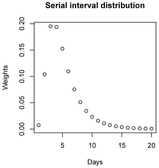
Figure 2.
Serial interval distribution. The discretized distribution of the serial interval for COVID-19 at the beginning of the pandemic with a mean equal to 4.7 days and standard deviation equal to 2.9 days.
The Poisson distribution is usually used to describe the distribution of the daily number of the infected [30,31]. In the Poisson distribution, the value of the population standard distribution is equal to the value of the population mean, which can induce a significant change in the range of the forecast interval when the value of the daily infected has changed. Thus, the Poisson distribution is not a good choice for the distribution of the daily incidence () in our system. The Poisson model is nested in the negative binomial model. Thus, the negative binomial distribution is a more flexible model better choice for the daily number of the infected in our system.
Inspired by Cori and Systrom [13,32], we assumed that follows a negative binomial distribution with the mean being and standard deviation being the empirical standard deviation calculated with the former seven-day incidence numbers. To avoid values that are too small due to the recording pattern, we use 200 as the standard deviation of the incidence number of COVID-19 when the empirical standard deviation is less than 200, and 50 as the lower bound of the standard deviation of the incidence number of H1N1 based on best performance. We expected that the reproduction number would not change drastically every day, and is assumed to follow a gamma distribution with the mean and standard deviation 0.003 based on best performance.
The conditional probability function can be represented as follows:
where , and is the empirical variance calculated with the former seven-day data. In addition, we have:
where and .
According to the Bayesian formula, we have:
which is a product of a negative binomial and a gamma distribution. With the posterior distribution and the Markov Chain Monte Carlo (MCMC) method, a simulation following the distribution of can be performed at time t, taking the mean of the simulation as the estimation of . We compared the value of with 1, and Alert 1 will be given when the value of is greater than 1, indicating that the infectious disease is in an outbreak period.
2.2.2. Prediction of and generation of Alert 2 or Note
Based on the estimation of , we calculate the joint distribution of and as follows:
The conditional probability functions of and can be gained easily by the similar probability functions of and .
The MCMC method was used again to simulate the joint distribution of and ; the mean of the simulation of and were considered as the prediction of and . Furthermore, the empirical 99.5% and 0.5% quantiles according to the simulation result were calculated as the upper and lower bounds of the 99% forecast interval for and , respectively.
At day t + 1, a comparison of the reported incidence value can be conducted with the simulated distribution of . Alert 2 and Note will be sent out according to the comparison result. There are three different situations as follows:
- (a)
- If the reported incidence value is in the forecast interval (0.5% quantile to 99.5% quantile), no mark will be sent out since the reported incidence value is within expectations.
- (b)
- If the reported incidence value is less than the lower bound (0.5% quantile), the Note will be given, which represents that the incidence number accidently decreases and the pandemic situation turns better.
- (c)
- If the reported incidence value is greater than the higher bound (99.5% quantile), the Alert 2 will be given, which represents that the incidence number accidently increases and the pandemic situation turns worse.
The corresponding marks will be given under situation b or c, when there is an abrupt change in the daily incidence number.
The alert marks, including Alert 1 and Alert 2, and the safe mark, Note, can give an intuition about the pandemic development to the audiences, which ideally can provide some instructions about travelling and self-protection strategies.
3. Results
We applied the detection and prediction system in several regions of the United States, Canada, Australia, UK, and Asia for COVID-19 as well as in Hong Kong for the H1N1 pandemic in 2009.
Many variants of the SARS-CoV-2 coronavirus have arisen during the pandemic. Some spread around the world, while others quickly disappeared and were replaced by other variants [33]. Alpha, Delta and Omicron are three dominant variants in most regions of the world in different time periods. There is no evidence that shows that Alpha (B.1.1.7) is associated with a change in serial intervals [34]. Thus, the serial interval distribution for Alpha we used in our system is the same as the one for COVID-19 at the beginning of the pandemic, which has a mean equal to 4.7 days and standard deviation equal to 2.9 days [28]. The Delta and Omicron variants have shorter serial intervals [35] compared with the former variants. We adopted the log normal distribution with a mean equal to 3.00 days and standard deviation equal to 2.48 days as the serial interval distribution for the Delta variant and the distribution with a mean equal to 2.75 days and standard deviation equal to 2.53 days for the Omicron variant [36].
In the United States, the Delta variant became the dominant variant during the summer of 2021, and the Omicron variant has now surpassed it as the dominant variant from the end of 2021 [37]. The dates that the Delta and Omicron variants became the dominant variants in the specific regions used in our system are shown in Table 1. The dates refer to the Covariant Platform [37]. We selected the dates from when the defined variant accounted for over 60% of the total number of sequences. For the states and cities among the United States, we used the Delta variant serial interval from 5 July 2021 to 3 January 2022, and we used the Omicron variant serial interval after 3 January 2022.

Table 1.
Date of the COVID-19 variants becoming dominant. The table shows the dates when the Delta and Omicron variants became the dominant variants in the specific region used in our system. The dates refer to the Covariant Platform [37]. We selected the dates from when the defined variant accounted for over 60% of the total number of sequences.
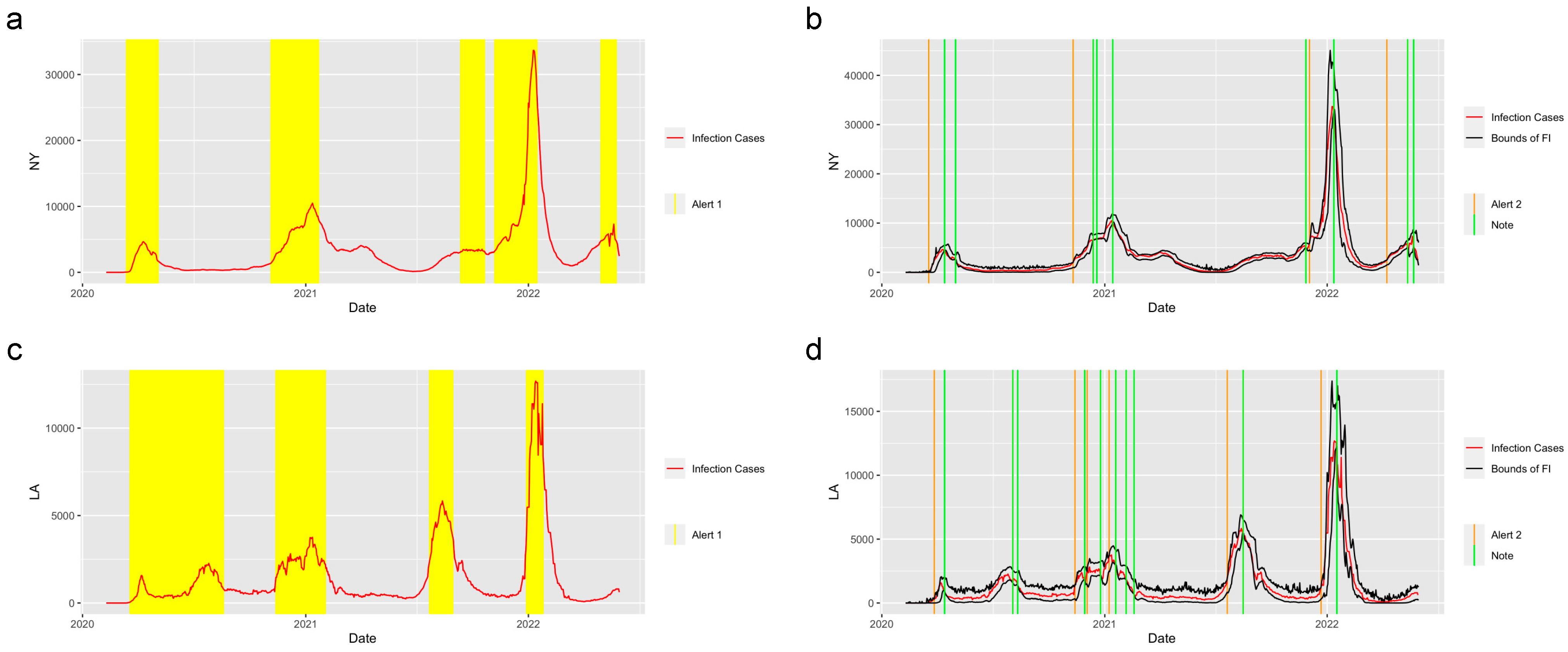
Figure 3 shows the prediction and detection system applied in the state of New York and the city of Los Angeles. There are three waves of COVID-19 that happened in New York and five waves that happened in Los Angeles. The system successfully detected the period of increasing, when the value of the reproduction number was greater than 1 and gave the Alert 1s at the increasing periods of each wave of COVID-19. The system captured the trend of the abrupt increase at the start of the increasing period in these two regions and gave the Alert 2s when the abrupt increases were detected. Moreover, the Notes successfully detected the potential abrupt decrease in the two regions.
Figure 3.
Alerts in NY and LA. The yellow and orange vertical lines represent Alert 1s and Alert 2s, correspondingly. The green vertical lines represent the Notes. The red lines represent the 7-day-average COVID-19 cases. The black lines represent the upper bound and lower bound of the forecast interval. During the period when the reproduction number is greater than 1, the Alert 1 will be given. (a,c) show the Alert 1s in NY and LA. When the reported infection case value is greater than the upper bound of the FI or smaller than the lower bound, the Alert 2 or Note will be given, correspondingly. (b,d) show the Alert 2s and Notes in NY and LA.
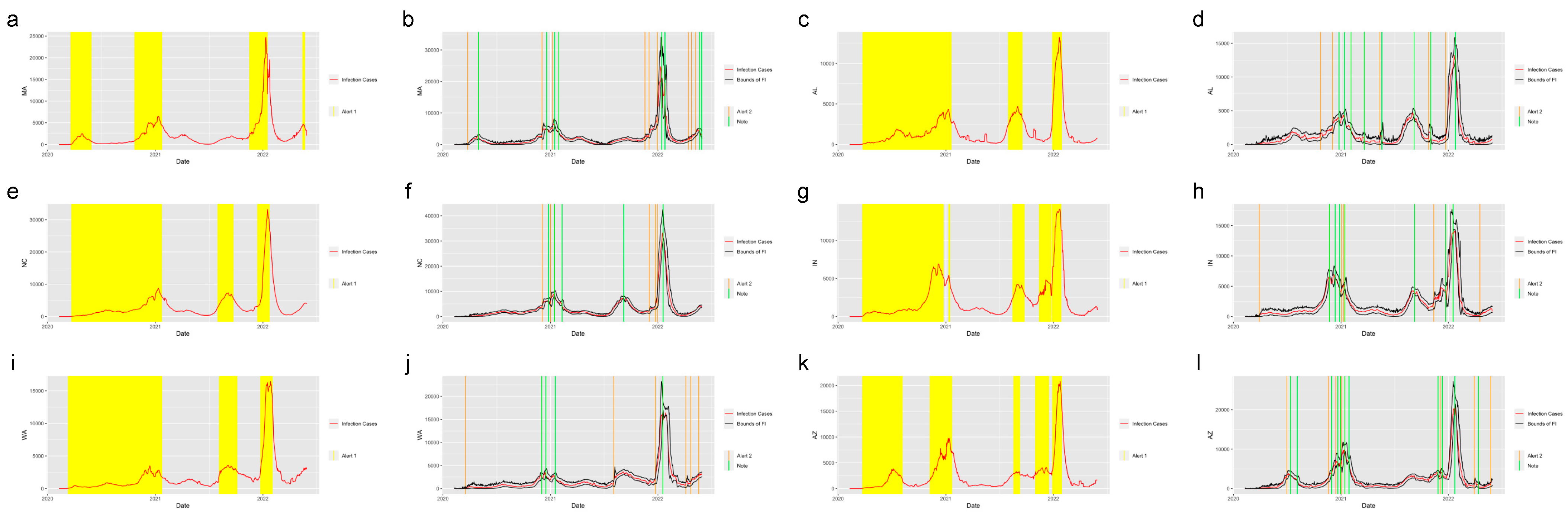
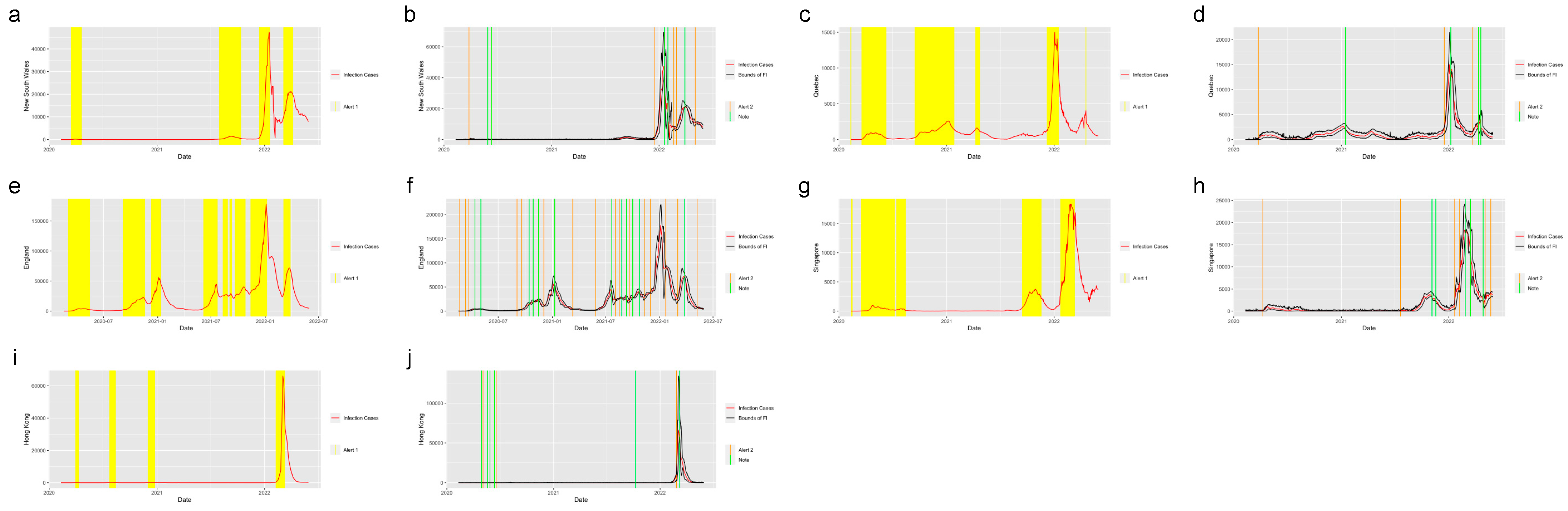
Figure 4 shows the system applied in the other six states in the United States. The six states were selected from five regions in the U.S.: Massachusetts (MA), which is from the Northeast Region; Alabama (AL) and North Carolina (NC) from the Southeast Region; Indiana (IN) from the Midwest; Washington State (WA) from the West and Arizona (AZ) from the Southwest. Figure 5 shows the system applied in the five regions outside the United States: New South Wales, Australia; Quebec, Canada; England, the United Kingdom; Singapore and Hong Kong. From the plots, we find that the system successfully detected the beginning of the waves and the increasing period for the regions in and out of the United States. The safe mark, Note, successfully showed the abrupt decrease in the different regions. This proves the effectiveness of the prediction and detection system in detecting the COVID-19 increasing and decreasing trends, which can provide the intuition of the development trend of the pandemic to residents, travelers and policy makers.
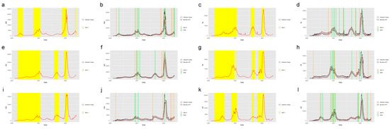
Figure 4.
Alerts in the states inside the United States. The yellow and orange vertical lines represent Alert 1s and Alert 2s, correspondingly. The green vertical lines represent the Notes. The red lines represent the 7-day-average COVID-19 cases. During the period when the reproduction number is greater than 1, the Alert 1 will be given. (a,c,e,g,i,k) show the Alert 1s in MA, AL, NC, IN, WA and AZ. When the reported infection case value is greater than the upper bound of the FI or smaller than the lower bound, the Alert 2 or Note will be given, correspondingly. (b,d,f,h,j,l) show the Alert 2s and Notes in MA, AL, NC, IN, WA and AZ.

Figure 5.
Alerts in the regions outside the United States. The yellow and orange vertical lines represent Alert 1s and Alert 2s, correspondingly. The green vertical lines represent the Notes. The red lines represent the 7-day-average COVID-19 cases. During the period when the reproduction number is greater than 1, the Alert 1 will be given. (a,c,e,g,i) show the Alert 1s in New South Wales, Quebec, England, Singapore and Hong Kong. When the reported infection case value is greater than the upper bound of the FI or smaller than the lower bound, the Alert 2 or Note will be given, correspondingly. (b,d,f,h,j) show the Alert 2s in New South Wales, Quebec, England, Singapore and Hong Kong.
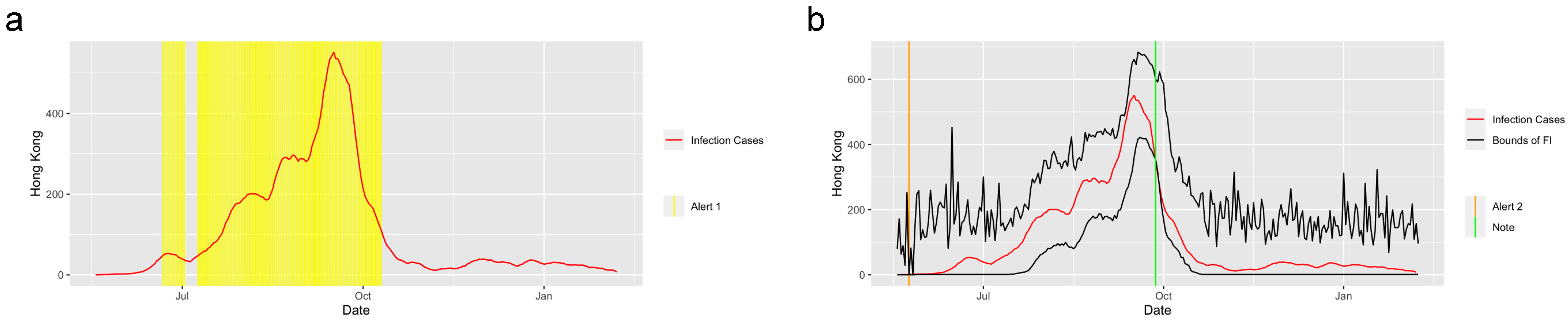
The system performed well in detecting the trend of other infectious diseases. Figure 6 shows the prediction and detection system for the H1N1 2009 pandemic applied in Hong Kong from 30 April 2009 to 7 February 2010. The system captured the trend of the abrupt increase at the start of the increasing period as well as the trend of abrupt decrease at the end of September 2010, and it successfully detected the period when the was greater than 1.
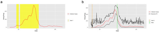
Figure 6.
Alerts in Hong Kong for the H1N1. The yellow and orange vertical lines represent Alert 1s and Alert 2s, correspondingly. The green vertical lines represent the Notes. The red lines represent the 7-day-average COVID-19 cases. During the period when the reproduction number is greater than 1, the Alert 1 will be given. (a) shows the Alert 1s in Hong Kong for the 2009 H1N1. When the reported infection case value is greater than the upper bound of the FI or smaller than the lower bound, the Alert 2 or Note will be given, correspondingly. (b) shows the Alert 2 and Note in Hong Kong for the 2009 H1N1.
4. Limitation
Due to limited data, we only applied our system in Hong Kong for H1N1. Furthermore, our system only considered the incidence number; however, there are other potential factors affecting pandemic development, including vaccine data, geographical location, population density, seasonality, temperature, etc. What is more, for some large regions such as California, our system did not perform well. We think the main reason is that California is highly heterogeneous and diversified with dense urban populations and spare rural areas; therefore, these and other factors will jointly affect the pandemic development. Further work will be conducted to examine how our system can be further improved including what grid size is optimal for reporting.
5. Discussion
The world may face other pandemics in the future. Thus, it is crucial to have a monitoring system to alert people to a pandemic outbreak as well as any drastic changes in its progression. In this study, we proposed a daily prediction and detection system structure of infectious diseases, which can accurately detect the abrupt increase in the incidence number of infectious diseases as well as the increasing period for the infectious diseases. Our system is not only applicable for the COVID-19 pandemic, but also for other infectious diseases such as the flu.
The daily incidence number can be misleading, in our judgement, of pandemic progress, as low incidence numbers do not absolutely represent a better pandemic situation. A low incidence number with an increasing trend can foretell danger down the road. Based on the Alert 1 mark, Alert 2 mark and the safe mark given by our prediction and detection system, users can infer more hidden information about pandemic progression and important activities, such as travelling, self-protection, etc., can be arranged accordingly.
As a prototype, we implemented our alert system online as a shiny app for the on-going COVID-19 pandemic for New York: https://guanchaotong.shinyapps.io/Covid-detection/ (accessed on 10 July 2023). We shall continuously expand our web-based alert system for other regions and other diseases to help fight this and other pandemics.
Author Contributions
Conceptualization, G.T., J.S. and W.Z.; Data Curation, J.S. and G.T.; Methodology, J.S., G.T. and W.Z.; Software, J.S. and G.T.; Validation, J.S., G.T. and W.Z.; Formal Analysis, J.S., G.T. and W.Z.; Investigation, J.S., G.T. and W.Z.; Resources, J.S., G.T. and W.Z.; Data Curation, J.S., G.T. and W.Z.; Writing—Original Draft Preparation, J.S., G.T. and W.Z.; Writing—Review and Editing, J.S., G.T. and W.Z.; Visualization, J.S., G.T. and W.Z. All authors have read and agreed to the published version of the manuscript.
Funding
This research received no external funding.
Institutional Review Board Statement
Not applicable.
Informed Consent Statement
Not applicable.
Data Availability Statement
The COVID-19 incidence number data of the states and cities in the United States analyzed in this study are openly available at the COVID Data Tracker: https://data.cdc.gov/api/views/9mfq-cb36/rows.csv (accessed on 25 June 2022). The COVID-19 incidence number data of England analyzed in this study are openly available at the UK Government website at: https://coronavirus.data.gov.uk/details/cases?areaType=nation&areaName=England (accessed on 28 June 2022). The COVID-19 incidence number data of Australia, Canada, Singapore and Hongkong analyzed in this study are openly available at the COVID-19 Data Repository by the Center for Systems Science and Engineering (CSSE) at Johns Hopkins University: https://github.com/CSSEGISandData/COVID-19 (accessed on 28 June 2022). The H1N1 incidence number data of Hong Kong analyzed in this study are openly available at https://plos.figshare.com/articles/dataset/_Early_real_time_estimation_of_the_basic_reproduction_number_of_emerging_or_reemerging_infectious_diseases_in_a_community_with_heterogeneous_contact_pattern_Using_data_from_Hong_Kong_2009_H1N1_Pandemic_Influenza_as_an_illustrative_example_/1545247/1 (accessed on 20 June 2022). The R codes used for the analysis and graphics of this paper are available upon request.
Conflicts of Interest
The authors declare no conflict of interest.
References
- You, C.; Deng, Y.; Hu, W.; Sun, J.; Lin, Q.; Zhou, F.; Pang, C.H.; Zhang, Y.; Chen, Z.; Zhou, X.-H. Estimation of the time-varying reproduction number of COVID-19 outbreak in China. Int. J. Hyg. Environ. Health 2020, 228, 113555. [Google Scholar] [CrossRef] [PubMed]
- Cucinotta, D.; Vanelli, M. WHO Declares COVID-19 a Pandemic. Acta Bio-Medica Atenei Parm. 2020, 91, 157–160. [Google Scholar] [CrossRef]
- WHO. WHO Coronavirus (COVID-19) Dashboard. Available online: https://covid19.who.int/ (accessed on 31 May 2022).
- Huang, C.; Wang, Y.; Li, X.; Ren, L.; Zhao, J.; Hu, Y.; Zhang, L.; Fan, G.; Xu, J.; Gu, X. Clinical features of patients infected with 2019 novel coronavirus in Wuhan, China. Lancet 2020, 395, 497–506. [Google Scholar] [CrossRef] [PubMed]
- Wang, D.; Hu, B.; Hu, C.; Zhu, F.; Liu, X.; Zhang, J.; Wang, B.; Xiang, H.; Cheng, Z.; Xiong, Y. Clinical characteristics of 138 hospitalized patients with 2019 novel coronavirus–infected pneumonia in Wuhan, China. JAMA 2020, 323, 1061–1069. [Google Scholar] [CrossRef] [PubMed]
- Deb, S.; Majumdar, M. A time series method to analyze incidence pattern and estimate reproduction number of COVID-19. arXiv 2020, arXiv:200310655. [Google Scholar]
- Wallinga, J.; Teunis, P. Different epidemic curves for severe acute respiratory syndrome reveal similar impacts of control measures. Am. J. Epidemiol. 2004, 160, 509–516. [Google Scholar] [CrossRef] [PubMed]
- Najafi, F.; Izadi, N.; Hashemi-Nazari, S.-S.; Khosravi-Shadmani, F.; Nikbakht, R.; Shakiba, E. Serial interval and time-varying reproduction number estimation for COVID-19 in western Iran. New Microbes New Infect. 2020, 36, 100715. [Google Scholar] [CrossRef] [PubMed]
- O’Driscoll, M.; Harry, C.; Donnelly, C.A.; Cori, A.; Dorigatti, I. A comparative analysis of statistical methods to estimate the reproduction number in emerging epidemics, with implications for the current coronavirus disease 2019 (COVID-19) pandemic. Clin. Infect. Dis. 2021, 73, e215–e223. [Google Scholar] [CrossRef]
- Wallinga, J.; Lipsitch, M. How generation intervals shape the relationship between growth rates and reproductive numbers. Proc. R. Soc. B Biol. Sci. 2007, 274, 599–604. [Google Scholar] [CrossRef]
- Kermack, W.O.; McKendrick, A.G. Contributions to the mathematical theory of epidemics–I. 1927. Bull. Math. Biol. 1991, 53, 33–55. [Google Scholar] [PubMed]
- White, L.F.; Wallinga, J.; Finelli, L.; Reed, C.; Riley, S.; Lipsitch, M.; Pagano, M. Estimation of the reproductive number and the serial interval in early phase of the 2009 influenza A/H1N1 pandemic in the USA. Influenza Other Respir. Viruses 2009, 3, 267–276. [Google Scholar] [CrossRef] [PubMed]
- Cori, A.; Ferguson, N.M.; Fraser, C.; Cauchemez, S. A new framework and software to estimate time-varying reproduction numbers during epidemics. Am. J. Epidemiol. 2013, 178, 1505–1512. [Google Scholar] [CrossRef]
- Gunzler, D.D.; Sehgal, A.R. Time-varying COVID-19 reproduction number in the United States. MedRxiv 2020. [Google Scholar] [CrossRef]
- He, W.; Yi, G.Y.; Zhu, Y. Estimation of the basic reproduction number, average incubation time, asymptomatic infection rate, and case fatality rate for COVID-19: Meta-analysis and sensitivity analysis. J. Med. Virol. 2020, 92, 2543–2550. [Google Scholar] [CrossRef]
- Linka, K.; Peirlinck, M.; Kuhl, E. The reproduction number of COVID-19 and its correlation with public health interventions. Comput. Mech. 2020, 66, 1035–1050. [Google Scholar] [CrossRef]
- Zhao, H.; Merchant, N.N.; McNulty, A.; Radcliff, T.A.; Cote, M.J.; Fischer, R.S.; Sang, H.; Ory, M.G. COVID-19: Short term prediction model using daily incidence data. PLoS ONE 2021, 16, e0250110. [Google Scholar] [CrossRef] [PubMed]
- Yang, H.; Sürer, Ö.; Duque, D.; Morton, D.P.; Singh, B.; Fox, S.J.; Pasco, R.; Pierce, K.; Rathouz, P.; Valencia, V.; et al. Design of COVID-19 staged alert systems to ensure healthcare capacity with minimal closures. Nat. Commun. 2021, 12, 3767. [Google Scholar] [CrossRef] [PubMed]
- Stevenson, F.; Hayasi, K.; Bragazzi, N.L.; Kong, J.D.; Asgary, A.; Lieberman, B.; Ruan, X.; Mathaha, T.; Dahbi, S.-E.; Choma, J.; et al. Development of an Early Alert System for an Additional Wave of COVID-19 Cases Using a Recurrent Neural Network with Long Short-Term Memory. Int. J. Environ. Res. Public. Health 2021, 18, 7376. [Google Scholar] [CrossRef]
- CDC. COVID Data Tracker. Centers for Disease Control and Prevention. 2022. Available online: https://covid.cdc.gov/covid-data-tracker (accessed on 25 June 2022).
- CDC. COVID Data Tracker Weekly Review. Centers for Disease Control and Prevention. 28 October 2022. Available online: https://www.cdc.gov/coronavirus/2019-ncov/covid-data/covidview/index.html (accessed on 29 October 2022).
- UK Government. Cases in England. 2022. Available online: https://coronavirus.data.gov.uk/details/cases?areaType=nation&areaName=England (accessed on 28 June 2022).
- Dong, E.; Du, H.; Gardner, L. An interactive web-based dashboard to track COVID-19 in real time. Lancet Infect. Dis. 2020, 20, 533–534. [Google Scholar] [CrossRef]
- Johns Hopkins University. COVID-19 Map. Johns Hopkins Coronavirus Resource Center. Available online: https://coronavirus.jhu.edu/map.html (accessed on 29 October 2022).
- On Kwok, K.; Davoudi, B.; Riley, S.; Pourbohloul, B. Age-specific daily count of reported pH1N1 (2009) cases in Hong Kong from April 30, 2009 to February 7, 2010. PLoS ONE 2015. [Google Scholar] [CrossRef]
- Fraser, C. Estimating individual and household reproduction numbers in an emerging epidemic. PLoS ONE 2007, 2, e758. [Google Scholar] [CrossRef] [PubMed]
- Feinleib, M. A Dictionary of Epidemiology, -Edited by John M. Last, Robert A. Spasoff, and Susan S. Harris. Am. J. Epidemiol. 2001, 154, 93–94. [Google Scholar] [CrossRef]
- Nishiura, H.; Linton, N.M.; Akhmetzhanov, A.R. Serial interval of novel coronavirus (COVID-19) infections. Int. J. Infect. Dis. 2020, 93, 284–286. [Google Scholar] [CrossRef] [PubMed]
- Levy, J.W.; Cowling, B.J.; Simmerman, J.M.; Olsen, S.J.; Fang, V.J.; Suntarattiwong, P.; Jarman, R.G.; Klick, B.; Chotipitayasunondh, T. The serial intervals of seasonal and pandemic influenza viruses in households in Bangkok, Thailand. Am. J. Epidemiol. 2013, 177, 1443–1451. [Google Scholar] [CrossRef]
- Ben Hassen, H.; Elaoud, A.; Ben Salah, N.; Masmoudi, A. A SIR-Poisson Model for COVID-19: Evolution and Transmission Inference in the Maghreb Central Regions. Arab. J. Sci. Eng. 2021, 46, 93–102. [Google Scholar] [CrossRef]
- Hakulinen, T.; Dyba, T. Precision of incidence predictions based on poisson distributed observations. Stat. Med. 1994, 13, 1513–1523. [Google Scholar] [CrossRef] [PubMed]
- Systrom, K.; Vladek, T.; Krieger, M. Rt.live. GitHub Repos. 2020. Available online: https://github.com/rtcovidlive/covid-model (accessed on 1 June 2022).
- Corum, J.; Zimmer, C. Tracking Omicron and Other Coronavirus Variants. The New York Times, 2021. Available online: https://www.nytimes.com/interactive/2021/health/coronavirus-variant-tracker.html(accessed on 25 June 2022).
- Geismar, C.; Fragaszy, E.; Nguyen, V.; Fong, W.L.E.; Shrotri, M.; Beale, S.; Rodger, A.; Lampos, V.; Byrne, T.; Kovar, J. Household serial interval of COVID-19 and the effect o f Variant B. 1.1. 7: Analyses from Prospective Community cohor t Study (Virus Watch). Wellcome Open Res. 2021, 6, 224. [Google Scholar] [CrossRef]
- Backer, J.A.; Eggink, D.; Andeweg, S.P.; Veldhuijzen, I.K.; van Maarseveen, N.; Vermaas, K.; Vlaemynck, B.; Schepers, R.; van den Hof, S.; Reusken, C.B. Shorter serial intervals in SARS-CoV-2 cases with Omicron BA. 1 variant compared with Delta variant, the Netherlands, 13 to 26 December 2021. Eurosurveillance 2022, 27, 2200042. [Google Scholar] [CrossRef] [PubMed]
- Kremer, C.; Braeye, T.; Proesmans, K.; André, E.; Torneri, A.; Hens, N. Observed serial intervals of SARS-CoV-2 for the Omicron and Delta variants in Belgium based on contact tracing data, 19 November to 31 December 2021. medRxiv 2022. [CrossRef]
- Hodcroft, E.B. CoVariants: SARS-CoV-2 Mutations and Variants of Interest. 2021. Available online: https://covariants.org/ (accessed on 25 June 2022).

Disclaimer/Publisher’s Note: The statements, opinions and data contained in all publications are solely those of the individual author(s) and contributor(s) and not of MDPI and/or the editor(s). MDPI and/or the editor(s) disclaim responsibility for any injury to people or property resulting from any ideas, methods, instructions or products referred to in the content. |
© 2023 by the authors. Licensee MDPI, Basel, Switzerland. This article is an open access article distributed under the terms and conditions of the Creative Commons Attribution (CC BY) license (https://creativecommons.org/licenses/by/4.0/).