Article

Utility in Time Description in Priority Best–Worst Discrete Choice Models: An Empirical Evaluation Using Flynn’s Data

Department of Mathematics and Statistics, Old Dominion University, Norfolk, VA 23529, USA
*
Author to whom correspondence should be addressed.
Stats 2024, 7(1), 185-202; https://doi.org/10.3390/stats7010012
Submission received: 8 January 2024 / Revised: 16 February 2024 / Accepted: 18 February 2024 / Published: 19 February 2024

Abstract

:
Discrete choice models (DCMs) are applied in many fields and in the statistical modelling of consumer behavior. This paper focuses on a form of choice experiment, best–worst scaling in discrete choice experiments (DCEs), and the transition probability of a choice of a consumer over time. The analysis was conducted by using simulated data (choice pairs) based on data from Flynn’s (2007) ‘Quality of Life Experiment’. Most of the traditional approaches assume the choice alternatives are mutually exclusive over time, which is a questionable assumption. We introduced a new copula-based model (CO-CUB) for the transition probability, which can handle the dependent structure of best–worst choices while applying a very practical constraint. We used a conditional logit model to calculate the utility at consecutive time points and spread it to future time points under dynamic programming. We suggest that the CO-CUB transition probability algorithm is a novel way to analyze and predict choices in future time points by expressing human choice behavior. The numerical results inform decision making, help formulate strategy and learning algorithms under dynamic utility in time for best–worst DCEs.

1. Introduction

Modelling choice behaviors has always been a very challenging part in statistical research. Best–worst scaling (BWs) choice pairs in model behaviors has been coined by Louviere and Woodworth (1990) [1]. With the addition of the attribute and attribute levels, the logistic distributions are convenient tools from analytic and practical aspects; they rely on assumptions of ordinality in the responses that can only be met under limited situations. Furthermore, the computational issues related to the large choices in the best–worst cases hamper patterns in the preferences. Discrete choice experiments (DCE) are one of popular models used to quantify the inspiration of attributes, which characterize the choice options. In the literature, Train (2009) [2] present multiple models based on different assumptions about the distribution of random components. In some of his suggested models, the error terms seem to be homogeneous and uncorrelated. Lancsar et al. (2013) [3] used a form of choice experiment, “Best–Worst Discrete Choice Experiments”, which is designed in a way by asking respondents to choose not only the best option in a choice set but also the worst option followed by the best from the remaining options and so on until the implied preference ordering of the option is obtained. Marley and Louviere (2005) [4] and Marley et al. (2008) [5] discuss some of the theoretical aspects of attribute-level best–worst experiments and Flynn et al. (2007) [6] provides detailed instructions for the analysis of such experiments. Following Marley et al. (2008) [5], Street and Knox (2012) [7] constructed a probability function called best–worst choice probability which can be used to find the probability of choice from one state to another. Working et al. (2018) [8] used a conditional logit approach to calculate the transition (of conditional choice) probabilities over time assuming that the consumer behavior is a time-dependent process. The assumption of “making two choices in two different time points is independent process for an individual” cannot be justified in general. As mentioned in Potoglou et al. (2011) [9], the interaction between attributes and choice pairs needs further piloting and investigation. The dependence in the modelling of the choices made over time is not fully included in many research venues. The dependence in the selection is a wide and fast field, but the theory is biased towards the estimation method. The premise of the traditional choice models assumes of mutually exclusive alternatives; that is, if a choice is made, alternates are not selected anymore. An alternative would be to build patterns of the preferences and their weighted measures. That option opens a new framework for choices, especially those that are made over time. Many factors shape the choices made. We include a priority in the selection over times and build it in the design. Specific association in the choices is highlighted to show the need to develop progressive models where temporal dependence in the choices is integrated, and utility is computed. In that sense, the innovation we propose is built under the copula theory, as it captures the dependence among the choices made over time periods irrespective of the marginal distributions. We utilized a completely new copula structure call ‘CO-CUB’ to calculate transition probabilities in the BWs choices over time.
The paper is organized as follows. In Section 2, DCMs are reviewed. The design for the BW choice pairs and their utilities are also included under a priority setting. The transition probabilities under CO-CUB are described in Section 3. We present the model’s theory overtime sequence to quantify and measure consumer behavior and derive utilities using the Markov decision process (MDPs) in Section 4. Section 5 is about the application. Empirical data from Flynn et al. (2007) [6] are simulated and our methods are tested, which have the ability to estimate selected significant parameters such as the “feeling” and “uncertainty” of human beings when making a choice. The literature on Copula for DCE is at its infancy by utilizing our newly constructed probability model to analyze the choices of individuals, comparisons are made, and we end up with a conclusion.

2. Preliminary Results for Best–Worst Discrete Choice Modelling

Best–worst scaling experiments are modified DCEs to elicit further information about the best and worst product, or best and worst attributes and attribute-levels of a product. Respondents are asked make choices between different attributes within a same product; that is the alternatives are the attributes. In the experiment, each of the alternatives is described by a set of K attributes or characteristics of the product or scenario being modelled. Further, each attribute contains l k levels. That is, each product is represented by a profile X = ( A 1 , A 2 , , A K ) ,   where A i represents an attribute level of a choice. Consider K profiles such that P 1 = A 11 , A 12 , , A 1 K , P 2 = A 21 , A 22 , , A 2 K , , P G = A G 1 , A G 2 , , A G K . For every profile, the choice set is then, C X = [ ( x 1 , x 2 ) , , ( x 1 , x K ) , ( x 2 , x 3 ) , ( x K 1 , x K ) , ( x 1 , x 2 ) , , ( x K , x K 1 ) ] ,   where the first attribute level is the best and the second is the worst, called best–worst pairs. This model is designed in such way that the choice pair ( x a , x b ) , x a , and x b cannot be acquired from the same attribute. From the choice set C X , the respondent determines a BW choice pair from τ such pairs, where τ = K ( K 1 ) . If we consider G products, that is, G profiles and G associated choice sets, then we can define a finite set S that is S = { C 1 , C 2 , , C G } such that C i C j for all i j . The BW choice pairs are illustrated in Figure 1 and shows all the possible combinations.
Total number of attribute levels
L = k = 1 K l k
and the total number of unique attribute-level pairs
Z = k = 1 K l k ( L l k ) ,  
where l k is the number of levels for k t h attribute, where 1 k K . Equation (1) is also described in Street and Knox (2012) [7].

2.1. Design of Experiment

Assume that the profiles have K attributes, and each attribute has l k levels, where k = 1 , 2 , , K . The simulation has performed in such a way that each person has to make choices in all sets. The debate concerning optimal designs for DCEs could be enhanced by a closer connection to the established literature on the optimal design of experiments as suggested in Sun et al. (2023) [10]. We used orthogonal design here for the simulation. There are three standard models in best–worst choice model design experiments which are: (1) paired, (2) marginal, and (3) marginal sequential models. In this manuscript, we used the paired model Aizaki and Fogarty (2019) [11] and Marley and Louviere (2005) [4], which assumes that the difference in utility between the two levels represents the greatest utility difference among all τ utility differences.

2.1.1. Paired Model with Attribute and Level Variables

Flynn et al. (2007) [6] used a paired model in his “Quality of life” analysis. In this approach, the attribute variables are created as dummy-coded variables (attribute-specific constants), with reversed signs when the attributes are treated as the worst and the level variables are created as effect coding with a base level for each attribute. The signs of the effect-coded level variables are also reversed when levels are treated as the worst. When estimating this model, an arbitrary attribute variable is omitted, and the coefficient of the omitted attribute variable is normalized to be zero. That is, the coefficients of the remaining attribute variables are estimated relative to the omitted attribute. Unlike dummy coding, effect coding allows the calculation of a coefficient of the base level in each attribute: it is the negative of the sum of the remaining coefficients in each attribute.
Let us consider the general scenario to the formulation for the paired model. Consider the K attributes A 1 , A 2 , , A K ; each has l k levels. Assume that attribute A K is omitted, and that the last level ( l k ) in each attribute (i.e., levels A 1 l k , A 2 l k ,   and A K l k ) is the base level. As in Aizaki and Fogarty (2019) [11], the systematic component of the utility function is then:
V = β A 1 M A 1 + + β A K 1 M A K 1 + β A 11 M A 11 + + β A 1 ( l k 1 ) M A 1 ( l k 1 ) + + β A K ( l k 1 ) M A K ( l k 1 ) ,
where the β s are the coefficients to be estimated and M s are the design matrices associated with the attributes and attribute levels. The coefficient of the attribute variable corresponding to A K is zero, and the coefficients of the base level A j l k , j = 1 , 2 , , K can be calculated by A j l k = i = 1 k 1 β A j i for j = 1 , 2 , , K . Detailed calculations are shown in the application section. M is composed of indicators for the best and worst attributes and attribute levels. Let M be the Z × P design matrix, where Z = k = 1 K l k L l k   and P = K l k 1 . Columns correspond to attribute A K and the base levels ( A 1 l k , A 2 l k ,   and A K l k ) are omitted from the design matrix. Consider the choice pair ( x i j , x i j ) from the choice set C i , for i = 1 , 2 , , G , j j = 1 , 2 , , K , and 1 x i j l k . For
M A h = { 1     ,   if   x i j   ϵ   A h   for   h = 1 , 2 , , K 1   1 , if   x i j   ϵ   A h   for   h = 1 , 2 , , K 1   0 ,                                         o t h e r w i s e
Let M A h x i h be the data for the attribute level 1 x i h l h ,     h = 1 , 2 , , K 1 (non-base levels) within attribute A J , j = 1 , 2 , , K . Referring to the choice pair ( x i j , x i j ) , the corresponding data for the attribute-levels are given by,
M A h x i h = { 1     ,   if   x i j   ϵ   A h   for   h = 1 , 2 , , K 1   1 , if   x i j   ϵ   A h   for   h = 1 , 2 , , K 1   0 ,     o t h e r w i s e .
Within attribute A J , j = 1 , 2 , , K , the base levels ( A 1 l k , A 2 l k ,   and A K l k )
M A 1 l k = M A 2 l k = = M A K l k = { 1   ,   if   x i j   ϵ   A K   1   , if   x i j   ϵ   A K   0 ,     o t h e r w i s e .
Table 1 shows the design matrix for the based on data from Flynn et al. (2007) [6] ‘Quality of Life experiment.’ The estimated parameters of the choices are given in Table 2. The BW choice pairs are then arranged according to their popularity (with highest number of picks) in Table 3.

2.2. Utility Function–Attribute–Level Best–Worst Design

The utility function as described in McFadden (1974) [12] for the i t h consumer/individual selecting the j t h choice is given as:
U i j = V i j + ε i j
where U i j is the utility for i t h consumer selecting j t h choice. V i j captures the systematic component and ε i j captures the error component. The distribution of the error terms is studied in McFadden (1974) [12]. He proposed the type I extreme value distribution (Gumbel distribution) for the error terms, which modelled data from the conditional logit model. However, this utility function can only accommodate single choice cases. Under the random utility theory, the probability of an alternative is based on the utility as defined in Equation (6); Flynn et al. (2007, 2008) [6,13] and Louviere et al. (2008) [14] provided the utility function for best–worst choice models. Here, we consider the choice set C , ( x i j , x i j ) being the chosen pair, and the utility for choosing this pair within set C is then given by:
U i j j = V i j j + ε i j j ,
where U i j j is the utility value for i t h consumer selecting j t h choice as the best and j t h as the worst. V i j j is the corresponding systematic component and ε i j j is the error term. The systematic component in Equation (7) can be calculated under the above-described paired model (Equation (2)).

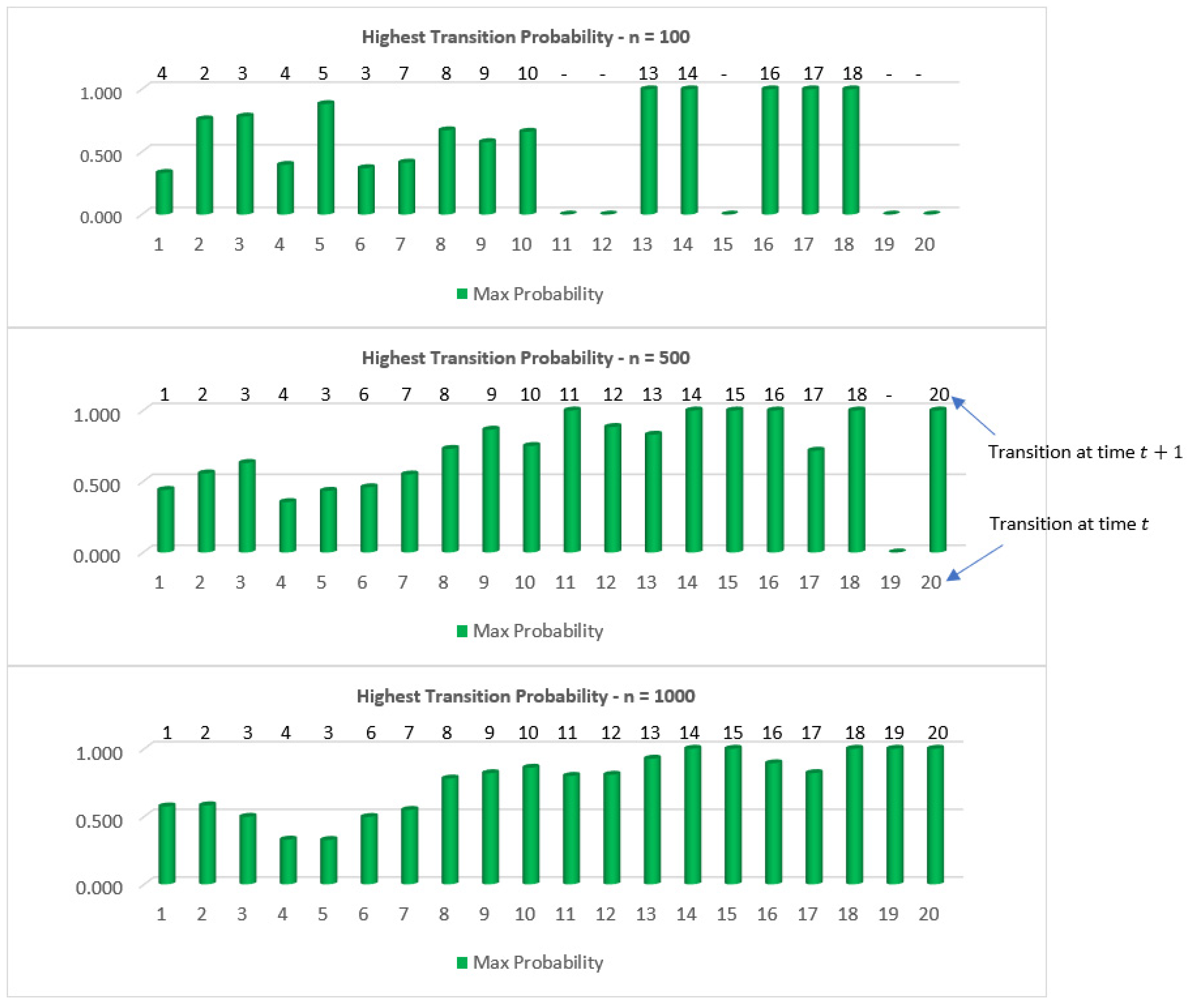
3. Transition Probability

In the context of choice models, we say that the choices are not independent of an irrelevant alternative (IIA) and they are also time dependent. Therefore, we may not achieve an accurate overall performance by not accounting for the relationship between the present and future decisions and their outcomes. Our interest is with discrete time finite horizon Markov Decision Processes (MDP); that is, t = 1 , 2 , T where T is a fixed number of time periods. The rewards are maximized by the best sequential decisions over time, making MDPs a dynamic optimization tool as used in Blanchet (2016) [15] to identify the right choices of substitution behaviors of consumers. Let s t S   be the states occupied at time t , r t ( s t ) which is the reward associated with s t , and d t   ( r t ,   s t ) is the decision based on the possible rewards and states at time t . The decision process maps the movement from one state to another over time t based on rewards received and an optimal decision set. As the decision process is Markovian, the transition probability to the next state, S = S t + 1 based solely on the decision made at the current state, S = S t is P S S = P [ S t + 1 = S | S t = S ] , where t = 1 , , T . The conditional probability of state transition from S to S is defined as:
P ( s t + 1 | s t ) = P ( s t + 1 = s | s t = s ) = P s s
The transition probability of state s is not homogeneous. As described in Equation (8), it depends on the action taken in the state S . Factors such as ‘feeling’ and ‘uncertainty’ of an individual can be highly affected to this probability. Further, the human behavior has a tendency to select options that have immediate gratification or those with the nearest range rather than selecting alternatives further away in time. Those are some of challenging constraints in terms of building a transition probability function. Further, the dependent structure of adjacent time probabilities needs to be handled carefully. Based on McFadden (1974) [12], the conditional logit model on the error term, Working et al. (2018) [7] establish a time-dependent probability formula while avoiding the IIA condition. It is reasonable as an initiation, but the dependent structure of the choice at the next time point or the above-mentioned ‘close at hand’ constraint cannot be seen in that transition matrix. In this manuscript, we introduced copula-based distribution with a CUB marginal, which is a combination of a discreet uniform and shifted binomial distributions introduced by Piccolo (2003) [16]. This model is a totally new approach for discrete choice modelling.

3.1. Copula Methods

Many stochastic models define the relation between X and Y through expectations, E ( Y | X = x ) = α + β x + ε . Copulas are functions that connect multivariate distributions to their one-dimensional margins. If F is an m -dimensional cumulative distribution function with one-dimensional margins, F 1 , , F d , then there exists an m -dimensional copula C such that F ( y 1 , , y d ) = C ( F 1 ( y 1 ) , , F d ( y d ) ) . The case d = 2 has attracted special attention; Trivedi and Zimmer (2005) [17]. Copula modelling demonstrates that practical implementation and estimation is relatively straightforward despite the complexity of its theoretical foundations. The copula approach for constructing joint distributions has gained popularity in recent years in applied research in finance, civil engineering, medicine, climate, and weather research and many more. Copula models have been widely used for modelling and characterizing dependence structure in multivariate data. The extension to handle discrete and continuous forms of data offers contingency to model the probability of best–worst pair selection probability.

3.2. CUB Probability Model

Piccolo (2003) [16], Piccolo and Simone (2019) [18], and D’Elia and Piccolo (2005) [19] introduce a radical model which is a Combination of a discrete Uniform and a shifted Binomial distribution (CUB). CUB jointly considers two latent components, called ‘feeling’ and ‘uncertainty’. General references for the statistical background for CUB are included in Iannario (2012) [20] and Iannario and Piccolo (2010) [21]. The stingy parameterization and the ease of estimation and interpretation make CUB models a very useful tool for choice data analyses. Piccolo and Simone (2019) [18] asserts that there is a possibility to fit statistical models to ordinal/choice data without the need of explanatory covariates. Our interest is to use CUB marginals for copula distribution to construct a transition probability matrix which can be used to identify human choice behavior in future time points, given the present state of choice. An interesting attempt at defining a bivariate CUB distribution using a multivariate model with fixed margins is made by Andreis and Ferrari (2013) [22]. The CUB is a class of mixture models, possibly involving covariates, developed as a new approach for modelling discrete choice processes. CUB models consider two components, which are the ‘uncertainty’ and ‘feeling’ of humans when making a choice. The intrinsic ‘uncertainty’ in choosing an item is modelled through a discrete uniform variable. The latent process leading to the choice is directed by the subjective ‘feeling’ and modelled using a shifted binomial distribution. The probability of observing a particular response r = 1 , 2 ,   m , with m known. Assuming m > 3 to ensure identifiability, the mixture probability model is described in Piccolo (2003) [16] and D’Elia and Piccolo (2005) [19]. It is given as:
P ( R = r | π , ξ ) = π ( m 1 r 1 ) ξ m r ( 1 ξ ) r 1 + ( 1 π ) 1 m   ;   r = 1 , 2 , , m ,
with π   ϵ   ( 0 ;   1 ] and ξ   ϵ   ( 0 ;   1 ] .
Here, π defines the weights of discrete uniform shifted binomial and it is inversely related to the amount of uncertainty in the choice decisions. The ξ is related to personal preferences and measures the strength of feeling. In CUB models, there is non-uniqueness of the copula representation and the non-uniqueness stems from the fact that marginal distribution functions, which are not strictly monotonically increasing, rather monotonically non-decreasing, do not possess an inverse in the usual sense, rather a pseudo-inverse; Nelsen (2007) [23], Genest et al. (2007) [24]. Because of that reason, we must be precisely cautioned when handling copulas with non-continuous margins, which is in the CUB model.

3.3. The CO-CUB Model (Copula-Based CUB)

Andreis and Ferrari (2013) [22] defines a multidimensional extension of CUB in Equation (9), called CO-CUB model, as a multivariate copula with discrete margins, each following a CUB distribution. A k -dimensional ( k   2 )   CO-CUB model with copula C is a multivariate discrete variable with margins R i   ~ C U B ( π i , ξ i ) ,   i = 1 , , k , each with support { 1 ,   , m i } ,   m i > 3 . Joint distribution function is given by:
Ψ ( r 1 , , r k , π _ , ξ _ , α _ ) = P ( R 1 r 1 , , R k r k , π _ , ξ _ , α _ ) = C α _ [ F 1 ( r 1 ; π 1 , ξ 1 ) , , F k ( r k ; π k , ξ k ) ] ,  
where π _ = ( π 1 , , π k ) and ξ _ = ( ξ 1 , , ξ k ) as in Equation (6), for a particular choice of copula C , characterized by a parameter α _ = ( α 1 , , α d ) taking values in some real d -dimensional space α defining the dependence structure of its components. F i ( r i ; π i , ξ i ) stands for the distribution function of the i t h margin; that is, F i ( r i ) = P ( R i r i ) and the support of the CO-CUB variable is the grid { 1 , , m 1 } × × { 1 , , m k } . The whole parameter set for a k -dimensional CO-CUB is, then, the ordered triplet ( π _ , ξ _ , α _ ) ϵ   [ 0 , 1 ] k × [ 0 , 1 ] k   ×   α , having the following interpretation: by the definition of copula, being margins of CUB, parameters ( π _ , ξ _ ) hold the same interpretation as in the unidimensional case, while for what concerns the copula parameter α _ , its interpretation as a dependence measure relates to the specific copula C adopted in Equation (10). Andreis and Ferrari (2013) [22] justified that the Placket copula distribution is one of the better candidates for the CO-CUB model.

3.4. The CO-CUB Model with Plackett Copula without Covariates

The Plackett copula is defined as:
C α ( u π 1 , ξ 1 , v π 2 , ξ 2 ) = A α ( u π 1 , ξ 1 , v π 2 , ξ 2 ) A α 2 ( u π 1 , ξ 1 , v π 2 , ξ 2 ) 4 α u π 1 , ξ 1 v π 2 , ξ 2 ( α 1 ) 2 ( α 1 ) , for   α ( 0 , 1 ) ( 1 , + ) ,
Here, u π 1 , ξ 1 = F 1 ( r 1 ) = i = 1 r 1 π 1 { ( m 1 1 i 1 ) ξ m 1 i ( 1 ξ 1 ) i 1 + ( 1 π 1 ) 1 m 1   } , where m 1 is the (fixed) number of categories of the first CUB model. This is similar for v π 2 , ξ 2 and we will from now on assume m 1 = m 2 = m > 3 . The copula probability mass function can be obtained as c α ( r 1 , r 2 ) = C α ( b 1 , b 2 ) C α ( a 1 , b 2 ) C α ( b 1 , a 2 ) + C α , where a i = F i ( r i ) and b i = F i ( r i 1 ) for i = 1, 2. Model parameters are then π 1 , ξ 1 , π 2 , ξ 2 and α . Estimation can be performed by inference for the margin method (IFM), as shown in Joe and Xu (1996) [25].

3.5. Setting up the Transition Probability Matrix

Let F ( x , y ) = C ( x , y ) be the cumulative function and f X Y ( x , y )   f X ( x ) f Y ( y ) = c ( u , v ) , where f Y = j | X = i = f ( y = j , x = i ) f ( x = i ) . Then, f Y | X = i = c ( u , v ) f Y ( y = j ) . For the notation convenient, let the choice state at time point t + 1 ,   s i ( t + 1 ) : = s i and the state at t ,   s i ( t ) : = s i , where s i , s i are ordered labels (ranks) of the BW choice pairs and s i , s i = 1 , 2 , , τ ; i = 1 , 2 , , G , and time t = 1 , 2 , , T . The transition probability is denoted as P i s s t = P t s i | s i . Since we do not have publicly available data from Flynn et al. (2007) [6] experiment, we have to simulate data under the paired model and distributed them among different choice sets. We simulated a number of different datasets under the same set of estimated regression parameters to prioritize choice pairs based on their popularity. That is, for a given choice set C , we counted the number of times an individual picked the choice pair   ( x i j , x i j ) . Finally, all the choices are arranged according to their popularity; that is, from the highest count to lowest count. This proceeding gave elements in a choice set, an ordinal power and it is a necessary requirement to incorporate the CUB model for choice data. Further, we adjusted the function for the repetition of selections in order to keep the transition probability formula as a probability distribution function. Then, the transition probability formula can be written as
c * ( u = g , v = h ) = { c ( u = g , v = h )   n C p   ; C p 0                               0           ; C p = 0
where n is the number of repetitions for a selection of the pair ( x i j , x i j ) in the selected choice set and C p = r = 1 N c ( u = g , v ) . I ( c ( u = g , v ) ) , c   is the density function of the Placket copula as shown in Equation (11). Let N be the size of the random sample, g ,   h = 1 , 2 , , τ , and τ be the number of BW choice pairs considered in each choice set. Then, the probability transition matrix for the i t h choice set is in the form of
c i * ( u = g , v = h ) = ( P i 11 P i 12 P i 1 τ P i 21 P i 22 P i 2 τ P i τ 1 P i τ 2 P i τ τ ) = ( P i s s ) i = 1 , 2 , , G ; ,   s ,   s = 1 , 2 , , τ = K ( K 1 ) .
P i s s is denoted as the transition probability when a consumer changing his choice selection state s at time t to s at time t + 1 . For all the transitions, s = 1 τ P i s s = 1 (e.g., the sum of the row values in Equation (13) is 1) and if there are no possible transitions s = 1 τ P i s s = 0 . The ordering scheme is such that for | s i s i | ω , P s s > P s s for any other s s for the i t h choice set, where ω is some small-time epoch number. That is, in simple words the row sum of the probability of the region | s i s i | ω   is the highest portion than any probability sum in the same row of the probability transition matrix in the i t h choice set. We introduce a constraint | s i s i | ω for our copula model because the nature of human behavior is that they have a greater tendency to grab options that are close at hand or those within the nearest range rather than picking up alternatives further away in time. The data were simulated based on that choice behavior assumption; that is, | s i s i | ω . The transition matrix may be either stationary or dynamic in nature. In this manuscript, we considered only the stationary case. It is important to state that the transition probability matrix is calculated by considering all N individuals in the experiment. The row sum of the transition matrix is kept as 0 if there is no transition from s to s . These proprieties can be seen in Table 4 and Table 5.

4. Utility in Time with Dynamic Programming

In this part, we incorporate MDPs and Dynamic Programming to calculate utility in time with the help of transition probabilities. Bellman (1954, 1956) [26,27] introduced a dynamic programming technique to evaluate the utility value function, also known as Bellman’s equation. At each time step, dynamic programming uses numerical methods to evaluate the value function moving backwards in time. Rust (1994, 2008) [28,29] and Ellickson (2011) [30] presented a numerical method with steps for evaluating DCEs as MDPs.
The value function for the DCEs is defined by at each time t as:
V t ( X t , ε t ) = max d t D t = t T P s s t ( γ t t U ( X t , d t ) + ε ( d t ) | X t ) ,
with P s s = P ( s t + 1 | s t ) = P ( s t + 1 = s | s t = s ) . This may also be defined in terms of the transition in decisions as P ( d t + 1 | d t , x t ) ,where d t D is the decision at time t ,     U ( x t   , d t ) is the derived expected utility, and ε is the associated error term at time t , where t = 1 ,   2 , ,   T . The discount utility rate in Equation (14) is given by γ ∈ (0, 1); see Feinberg and Schwartz (1994) [31]. There exist τ value functions for each of the τ alternatives in the experiments evaluated at each time point t = 1 ,   2 , ,   T . The sum goes from t up to T because it is evaluated using a backwards recursive method; that is, we start at the last time point and work our way backwards to earlier time points.
V T ( X T ) = U ( X T , d T ) V T 1 ( X T 1 , d T 1 ) = U ( X T 1 , d T 1 ) + d t D   γ V T ( X T ) P ( d T | d T 1 ) , V T 2 ( X T 2 , d T 2 ) = U ( X T 2 , d T 2 ) + d t D   γ V T 1 ( X T 1 ) P ( d T 1 | d T 2 ) , V t ( X t , d t ) = U ( X t , d t ) + t = t + 1 T d t D   γ V t ( X t ) P ( d t | d t ) ,
where U t is utility in time (UiT) and V t is the value function. Based on Working et al. (2018) [8], the initial utility for the selected choice pair can be calculated using:
V T = ( ( β ^ A + β ^ A k ) ( β ^ A + β ^ A k ) ) U ( X T , d T ) ,
where β ^ A , β ^ A k are estimated parameters for best attribute and attribute level and β ^ A , β ^ A k are the estimated parameters for worst attribute and attribute level, respectively. Instead of this simple model, in this manuscript we used the paired model which is one of the more appropriate models for the paired data. In fact, to distribute the utility over time for the future time points, further adjustment is needed for the value function. We adjusted the value function in Equation (12) for the time in such a way that
V T = ( M + β ^ ) θ b t + ( M β ^ ) θ w t U ( X T , d T ) ,   where   M = M + + M
M is the design matrix under the paired model which contains +1, −1, and 0 described in Equations (3)–(5). We broke M into M + and M , which contains + 1 s and 1 s. Further, we introduce arbitrary time-sensitive constants θ b t , θ w t to make the initial systematic component vary with time.

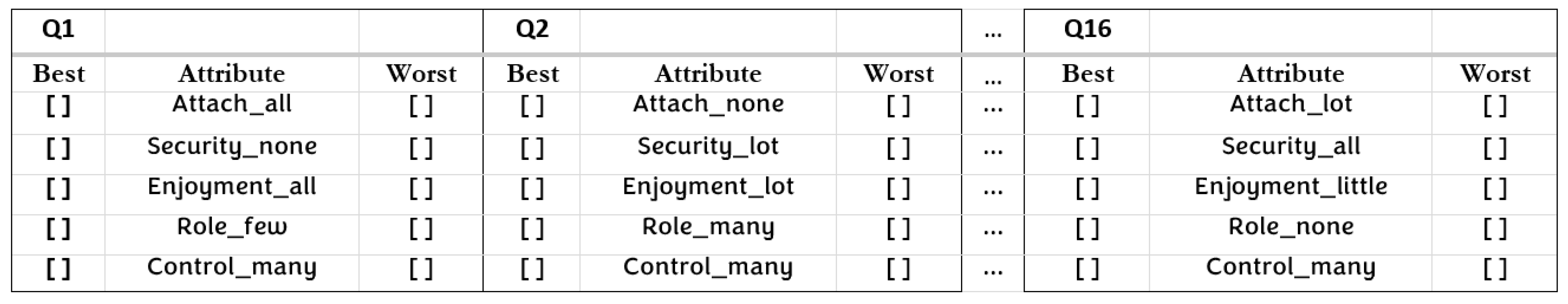
5. Application and the Design of the Experiment

A pilot best–worst study was conducted in summer 2005 among people aged 65 and over with the aim of informing a larger quality of life valuation exercise by Flynn et al. (2007) [6]. In this survey, there are K = 5   attributes, which are Attachment, Security, Role, Enjoyment, and Control. Each attribute with l k = 4 levels. That is
  • Attachment: Attach_none, Attach_little, Attach_lot, Attach_all
  • Security: Security_none, Security_little, Security_lot, Security_all
  • Role: Enjoyment_none, Enjoyment_little, Enjoyment_lot, Enjoyment_all
  • Enjoyment: Role_none, Role_few, Role_many, Role_all
  • Control: Control_none, Control_few, Control_many, Control_all
We simulated a new data set for 100 individuals and estimated regression parameters by using a conditional logit model with the help of R package ‘support.BWS2’; see Aizaki and Fogarty (2019) [11]. The application is from a balance design where all five attributes have four- levels each; there are 320 unique BW choice pairs. We simulated data in such a way that 16 choice sets were used to cage all 320 unique BW choice pairs (see Equation (1)), by keeping each choice set with 20 choice pairs. Each person of the 100 sample should make a choice in each choice set. Figure 2 shows the orthogonal design we used to simulate the data. The shape of the questionnaire design based on the orthogonal array is shown in Figure 3. Such a questionnaire could be used in the case of a real-life data collection process. Table 1 shows the design matrix for the paired model. The attribute ‘Control’ is omitted and the fourth level in each attribute (‘Attach_all’, ‘Security_all’, ‘Enjoyment_all’, ‘Role_all’ and ‘Control_all’) is considered to be the base level.
The parameter estimated by Flynn et al. (2007) [6] and conditional logit regression estimates for the simulation are presented in Table 2. Based on Equation (17), systematic components for each choice and then the corresponding utility can be calculated. Estimations for base levels are calculated by A j l k = i = 1 k 1 β A j i as mentioned in Section 2.1.1. As per the iterative dynamic programming method introduced in Equation (15), with initial utility as described in Equation (16), utility values for a consecutive 10 time periods are calculated recursively by utilizing the transition probabilities and a discount factor γ = 0.95. As a demonstration, the results for choice set 1 is presented in this manuscript.
The BW choice pairs are arranged in order, as mentioned in Section 3.4. We ran the choice selections algorithm 10,000 times within each choice set to get a proper ordering of elements. Table 3 shows the arrangement for the BW pairs for choice set 1. This arrangement is organized according to the popularity (highest number of picks) of the BW choice pairs. That information is then used to calculate the transition probabilities at the next time point. The probability transition matrix can be calculated utilizing our new model as derived in Equation (12). It is a 20 × 20 matrix since each choice sets contain 20 choice pairs. Figure 4 shows the highest probability corresponding to each BW choice pair in choice set 1 for three different samples sizes, which n = 100 , n = 500 , and n = 1000; that is, the highest probable transition slot at time t to t + 1. Table 4, Table 5 and Table 6 show the corresponding transition probability matrices for choice set 1 for sample sizes 100, 500, and 1000, respectively. The constraint region, |si’ − si| ≤ 3, is highlighted in the probability transition matrix and the highest probability is squared. Nobody picked choice pairs 11, 12, 15, 19, and 20 at time t or t + 1 when n = 100. That has happened only to choice pair 19 in the n = 500 scenario. However, for n = 1000 all the choice pairs have been selected. Table 7 shows the utilities (UiT) calculated for time points t = 1, 2,…, 10. Figure 5 shows the utility–time distribution of selected choices pairs (2, 7, 14, 16, and 18) in choice set 1. It highlights the dynamic utility in time.

6. Conclusions

In general, the choices are made at different time points and are not IIA for any individual. They depend on not only qualitative factors such as priority setting, feeling, and uncertainty, but also quantitative covariates such as measure of sequential selection probability in the process. By considering a specific popular model, we capture and monitor the dependent structure and calculate the transition probability between consecutive choices at adjacent time points. We were able to include parameters like feeling and uncertainty to the model. This new approach to calculating transition probabilities extend the ideas proposed by Piccolo (2003) [16] and Piccolo et al. (2019) [32]. Further, we could justify our initial assumption of the human choice behavior of | s i s i | ω , that they have a greater tendency to grab options that are close at hand or those within the nearest range rather than picking up alternatives further away in time.
Data to quantify the BW in the DCE models are mainly found outside of academia. In this paper, we have simulated the data. Such an issue is one limitation of the paper, but the approach has the advantage of bringing and completing the ranking. The paper could also gain if more covariates were given. Based on Flynn’s ‘Quality of life experiment’, we choose value ω as 3. The accuracy of the CO-CUB model can be further improved relaxing that constraint and by adding more latent covariates and updating knowledge of the ranking labels of the choice pairs within the choice set. We leave such ideas for future research.

Author Contributions

Conceptualization, S.A. and N.D.; methodology, S.A. and N.D.; software, S.A. and N.D.; validation, S.A. and N.D.; formal analysis, S.A. and N.D.; investigation, S.A. and N.D.; data curation, S.A. and N.D.; writing—original draft preparation, S.A. and N.D.; writing—review and editing, S.A. and N.D.; All authors have read and agreed to the published version of the manuscript.

Funding

This research received no external funding.

Data Availability Statement

Data was simulated.

Conflicts of Interest

The authors declare no conflict of interest.

References

  1. Louviere, J.J.; Woodworth, G.G. Best Worst Scaling: A Model for Largest Difference Judgments; Working Paper; Faculty of Business, University of Alberta: Edmonton, AB, Canada, 1990. [Google Scholar]
  2. Train, K.E. Discrete Choice Methods with Simulation; Cambridge University Press: Cambridge, UK, 2009. [Google Scholar]
  3. Lancsar, E.; Louviere, J.; Donaldson, C.; Currie, G.; Burgess, L. Best worst discrete choice experiments in health: Methods and an application. Soc. Sci. Med. 2013, 76, 74–82. [Google Scholar] [CrossRef]
  4. Marley, A.A.; Louviere, J.J. Some probabilistic models of best, worst, and best–worst choices. J. Math. Psychol. 2005, 49, 464–480. [Google Scholar] [CrossRef]
  5. Marley, A.A.J.; Flynn, T.N.; Louviere, J.J. Probabilistic models of set-dependent and attribute-level best–worst choice. J. Math. Psychol. 2008, 52, 281–296. [Google Scholar] [CrossRef]
  6. Flynn, T.N.; Louviere, J.J.; Peters, T.J.; Coast, J. Best–worst scaling: What it can do for health care research and how to do it. J. Health Econ. 2007, 26, 171–189. [Google Scholar] [CrossRef]
  7. Street, D.J.; Knox, S.A. Designing for attribute-level best-worst choice experiments. J. Stat. Theory Pract. 2012, 6, 363–375. [Google Scholar] [CrossRef]
  8. Working, A.; Alqawba, M.; Diawara, N.; Li, L. Time Dependent Attribute-Level Best Worst Discrete Choice Modelling. Big Data Inf. Anal. 2018, 3, 55–72. [Google Scholar] [CrossRef]
  9. Potoglou, D.; Burge, P.; Flynn, T.; Netten, A.; Malley, J.; Forder, J.; Brazier, J.E. Best–worst scaling vs. discrete choice experiments: An empirical comparison using social care data. Soc. Sci. Med. 2011, 72, 1717–1727. [Google Scholar] [CrossRef]
  10. Sun, T.; Chen, H.; Gao, Y.; Xiang, Y.; Wang, F.; Ni, Z.; Wang, X.; Huang, X. Best-Worst Scaling Survey of Inpatients’ Preferences in Medical Decision-Making Participation in China. Healthcare 2023, 11, 323. [Google Scholar] [CrossRef] [PubMed]
  11. Aizaki, H.; Fogarty, J. An R package and tutorial for case 2 best–worst scaling. J. Choice Model. 2019, 32, 100171. [Google Scholar] [CrossRef]
  12. McFadden, D. Conditional logit analysis of qualitative choice behavior. Front. Econom. 2005, 1, 7–32. [Google Scholar]
  13. Flynn, T.N.; Louviere, J.J.; Peters, T.J.; Coast, J. Estimating preferences for a dermatology consultation using best-worst scaling: Comparison of various methods of analysis. BMC Med. Res. Methodol. 2008, 8, 76. [Google Scholar] [CrossRef] [PubMed]
  14. Louviere, J.J.; Street, D.; Burgess, L.; Wasi, N.; Islam, T.; Marley, A.A. Modeling the choices of individual decision-makers by combining efficient choice experiment designs with extra preference information. J. Choice Model. 2008, 1, 128–164. [Google Scholar] [CrossRef]
  15. Blanchet, J.; Gallego, G.; Goyal, V. A Markov chain approximation to choice modeling. Oper. Res. 2016, 64, 886–905. [Google Scholar] [CrossRef]
  16. Piccolo, D. On the moments of a mixture of uniform and shifted binomial random variables. Quad. Di Stat. 2003, 5, 85–104. [Google Scholar]
  17. Trivedi, P.K.; Zimmer, D.M. 2 copulas and dependence. Found. Trends Econom. 2005, 1, 7–32. [Google Scholar]
  18. Piccolo, D.; Simone, R.; Iannario, M. Cumulative and CUB models for rating data: A comparative analysis. Int. Stat. Rev. 2019, 87, 207–236. [Google Scholar] [CrossRef]
  19. D’Elia, A.; Piccolo, D. A mixture model for preferences data analysis. Comput. Stat. Data Anal. 2005, 49, 917–934. [Google Scholar] [CrossRef]
  20. Innario, M. CUBE models for interpreting ordered categorical data with overdispersion. CUBE Models Interpret. Ordered Categ. Data Overdispersion 2012, 14, 137–140. [Google Scholar]
  21. Iannario, M.; Piccolo, D. A new statistical model for the analysis of customer satisfaction. Qual. Technol. Quant. Manag. 2010, 7, 149–168. [Google Scholar] [CrossRef]
  22. Andreis, F.; Ferrari, P.A. On a copula model with CUB margins. Quad. Di Stat. 2013, 15, 33–51. [Google Scholar]
  23. Nelsen, R.B. An Introduction to Copulas; Springer Science & Business Media: Berlin/Heidelberg, Germany, 2007. [Google Scholar]
  24. Genest, C.; Nešlehová, J. A primer on copulas for count data. ASTIN Bulletin J. IAA 2007, 37, 475–515. [Google Scholar] [CrossRef]
  25. Joe, H.; Xu, J.J. The Estimation Method of Inference Functions for Margins for Multivariate Models. 1996. Available online: https://open.library.ubc.ca/soa/cIRcle/collections/facultyresearchandpublications/52383/items/1.0225985 (accessed on 15 February 2024).
  26. Bellman, R. The theory of dynamic programming. Bull. Am. Math. Soc. 1954, 60, 503–515. [Google Scholar] [CrossRef]
  27. Bellman, R. Dynamic programming and Lagrange multipliers. Proc. Natl. Acad. Sci. USA 1956, 42, 767–769. [Google Scholar] [CrossRef] [PubMed]
  28. Rust, J. Structural estimation of Markov decision processes. Handb. Econom. 1994, 4, 3081–3143. [Google Scholar]
  29. Rust, J. Dynamic programming. New Palgrave Dict. Econ. 2008, 1, 8. [Google Scholar]
  30. Ellickson, P.B.; Misra, S. Structural workshop paper—Estimating discrete games. Mark. Sci. 2011, 30, 997–1010. [Google Scholar] [CrossRef]
  31. Feinberg, E.A.; Shwartz, A. Markov decision models with weighted discounted criteria. Math. Oper. Res. 1994, 19, 152–168. [Google Scholar] [CrossRef]
  32. Piccolo, D.; Simone, R. The class of CUB models: Statistical foundations, inferential issues and empirical evidence. Stat. Methods Appl. 2019, 28, 389–435. [Google Scholar] [CrossRef]
Figure 1. BW Choice pairs in G choice sets, Working et al. (2018) [8].
Stats 07 00012 g001
Figure 2. Orthogonal design for Flynn’s experiment flow chart of the 5 attributes, each with 4 levels, with 16 choice sets: e.g., A4 is the 1st attribute at the 4th level.
Stats 07 00012 g002
Figure 3. Questionnaire design based on the Orthogonal Array.
Stats 07 00012 g003
Figure 4. Most probable transition slots from time t to t + 1 .
Stats 07 00012 g004
Figure 5. Utility–Time graph for some selected BW choice pairs in choice set 1.
Stats 07 00012 g005
Table 1. Design Matrix based on Equations (3)–(5).
BW M A M B M C M D M A 1 M A 2 M A 3 M B 1 M B 2 M B 3 M C 1 M C 2 M C 3 M D 1 M D 2 M D 3 M E 1 M E 2 M E 3
A 3 D 2 1 0 0 1 0 0 1 0 0 0 0 0 0 0 1 0 0 0 0
A 1 B 3 1 1 0 0 1 0 0 0 0 1 0 0 0 0 0 0 0 0 0
E 3 C 3 0 0 1 0 0 0 0 0 0 0 0 0 1 0 0 0 0 0 1
A 2 C 4 1 0 1 0 0 1 0 0 0 0 1 1 1 0 0 0 0 0 0
D 2 E 3 0 0 0 1 0 0 0 0 0 0 0 0 0 0 1 0 0 0 1
A 1 B 4 1 1 0 0 1 0 0 1 1 1 0 0 0 0 0 0 0 0 0
A 4 B 2 1 1 0 0 1 1 1 0 1 0 0 0 0 0 0 0 0 0 0
A 1 E 4 1 0 0 0 1 0 0 0 0 0 0 0 0 0 0 0 1 1 1
E 4 A 4 1 0 0 0 1 1 1 0 0 0 0 0 0 0 0 0 1 1 1
Table 2. Estimated parameters.
Parameters β ^ F l y n n S E F l y n n β ^ S i m S E S i m Parameters β ^ F l y n n S E F l y n n β ^ S i m S E S i m
Constant−0.30670.075** Security All0.9511*0.8199*
Attachment0.81050.08030.86550.0575 Enjoyment None−0.88880.1286−0.83270.0759
Security**** Enjoyment Little−0.33670.1632−0.35350.0773
Enjoyment0.26320.1010.26840.0563 Enjoyment Lot0.65610.14930.58620.0781
Role0.19080.09740.22940.0565 Enjoyment All0.5695*0.60007*
Control0.10760.09710.12170.0564 Role None−0.89560.1239−0.76970.0761
Attachment_None−1.96780.1129−1.96330.0775 Role Few−0.02770.15320.10860.0776
Attachment_Little0.16940.10120.18110.0756 Role Many0.44350.13630.26160.0784
Attachment_Lot0.90530.09051.04930.0811 Role All0.4798*0.3995
Attachment_All0.8932*0.7329* Control None−0.80850.1122−0.71490.0763
Security_None−0.61230.118−0.69530.0764 Control Few0.08350.15960.15050.0774
Security Little−0.37610.1302−0.24490.077 Control Many0.2780.13760.28540.0785
Security Lot0.03730.11530.12030.0779 Control All0.4471*0.2791*
β ^ F l y n n —Estimated parameters from Flynn’s experiment. β ^ S i m —Estimated parameters from the simulation. The * represent the base levels in our simulated data.
Table 3. Arrangement of BW choice pairs in choice set 1, based on their popularity.
Best AttributeWorst AttributeBest LevelWorst LevelNo. of PicksRank
AttachmentSecurityAttach_allSecurity_none26291
AttachmentRoleAttach_allRole_few12042
EnjoymentSecurityEnjoyment_allSecurity_none10753
AttachmentControlAttach_allControl_many9944
ControlSecurityControl_manySecurity_none7005
AttachmentEnjoymentAttach_allEnjoyment_all6296
RoleSecurityRole_fewSecurity_none5097
EnjoymentRoleEnjoyment_allRole_few4988
EnjoymentControlEnjoyment_allControl_many4009
ControlRoleControl_manyRole_few34110
RoleControlRole_fewControl_many20611
ControlEnjoymentControl_manyEnjoyment_all16212
SecurityRoleSecurity_noneRole_few13013
RoleEnjoymentRole_fewEnjoyment_all12214
EnjoymentAttachmentEnjoyment_allAttach_all11715
SecurityControlSecurity_noneControl_many8916
ControlAttachmentControl_manyAttach_all6217
SecurityEnjoymentSecurity_noneEnjoyment_all5818
RoleAttachmentRole_fewAttach_all5119
SecurityAttachmentSecurity_noneAttach_all2420
Table 4. Probability transition matrix for choice set 1; ( n = 100 ) .
(   P i s s ) =
1234567891011121314151617181920
10.1890.2260.2520.3320.0000.0000.0000.0000.0000.0000.0000.0000.0000.0000.0000.0000.0000.0000.0000.000
20.0580.7600.0000.1150.0670.0000.0000.0000.0000.0000.0000.0000.0000.0000.0000.0000.0000.0000.0000.000
30.0340.0850.7830.0000.0620.0360.0000.0000.0000.0000.0000.0000.0000.0000.0000.0000.0000.0000.0000.000
40.0160.1600.3690.3970.0580.0000.0000.0000.0000.0000.0000.0000.0000.0000.0000.0000.0000.0000.0000.000
50.0000.0000.0000.0000.8820.0000.0000.1180.0000.0000.0000.0000.0000.0000.0000.0000.0000.0000.0000.000
60.0000.0000.3710.0000.1770.3110.0000.1420.0000.0000.0000.0000.0000.0000.0000.0000.0000.0000.0000.000
70.0000.0000.0000.2690.1590.0930.4150.0640.0000.0000.0000.0000.0000.0000.0000.0000.0000.0000.0000.000
80.0000.0000.0000.0000.0000.3270.0000.6730.0000.0000.0000.0000.0000.0000.0000.0000.0000.0000.0000.000
90.0000.0000.0000.0000.0000.4210.0000.0000.5790.0000.0000.0000.0000.0000.0000.0000.0000.0000.0000.000
100.0000.0000.0000.0000.0000.0000.0000.0000.0000.6610.3390.0000.0000.0000.0000.0000.0000.0000.0000.000
110.0000.0000.0000.0000.0000.0000.0000.0000.0000.0000.0000.0000.0000.0000.0000.0000.0000.0000.0000.000
120.0000.0000.0000.0000.0000.0000.0000.0000.0000.0000.0000.0000.0000.0000.0000.0000.0000.0000.0000.000
130.0000.0000.0000.0000.0000.0000.0000.0000.0000.0000.0000.0001.0000.0000.0000.0000.0000.0000.0000.000
140.0000.0000.0000.0000.0000.0000.0000.0000.0000.0000.0000.0000.0001.0000.0000.0000.0000.0000.0000.000
150.0000.0000.0000.0000.0000.0000.0000.0000.0000.0000.0000.0000.0000.0000.0000.0000.0000.0000.0000.000
160.0000.0000.0000.0000.0000.0000.0000.0000.0000.0000.0000.0000.0000.0000.0001.0000.0000.0000.0000.000
170.0000.0000.0000.0000.0000.0000.0000.0000.0000.0000.0000.0000.0000.0000.0000.0001.0000.0000.0000.000
180.0000.0000.0000.0000.0000.0000.0000.0000.0000.0000.0000.0000.0000.0000.0000.0000.0001.0000.0000.000
190.0000.0000.0000.0000.0000.0000.0000.0000.0000.0000.0000.0000.0000.0000.0000.0000.0000.0000.0000.000
200.0000.0000.0000.0000.0000.0000.0000.0000.0000.0000.0000.0000.0000.0000.0000.0000.0000.0000.0000.000
Table 5. Probability transition matrix for choice set 1; ( n = 500 ) .
( P i s s ) =
1234567891011121314151617181920
10.4410.2660.1780.1160.0000.0000.0000.0000.0000.0000.0000.0000.0000.0000.0000.0000.0000.0000.0000.000
20.1010.5570.1970.1120.0330.0000.0000.0000.0000.0000.0000.0000.0000.0000.0000.0000.0000.0000.0000.000
30.1130.1710.6310.0460.0120.0260.0000.0000.0000.0000.0000.0000.0000.0000.0000.0000.0000.0000.0000.000
40.1890.1910.2190.3550.0220.0160.0070.0000.0000.0000.0000.0000.0000.0000.0000.0000.0000.0000.0000.000
50.0000.0760.4340.0830.3770.0160.0000.0150.0000.0000.0000.0000.0000.0000.0000.0000.0000.0000.0000.000
60.0000.0000.2630.0750.1210.4590.0000.0530.0270.0000.0000.0000.0000.0000.0000.0000.0000.0000.0000.000
70.0000.0000.0000.2040.1460.0520.5490.0480.0000.0000.0000.0000.0000.0000.0000.0000.0000.0000.0000.000
80.0000.0000.0000.0000.0530.0370.0340.7300.0710.0370.0380.0000.0000.0000.0000.0000.0000.0000.0000.000
90.0000.0000.0000.0000.0000.0910.0000.0000.8650.0440.0000.0000.0000.0000.0000.0000.0000.0000.0000.000
100.0000.0000.0000.0000.0000.0000.0780.0000.0000.7500.1710.0000.0000.0000.0000.0000.0000.0000.0000.000
110.0000.0000.0000.0000.0000.0000.0000.0000.0000.0001.0000.0000.0000.0000.0000.0000.0000.0000.0000.000
120.0000.0000.0000.0000.0000.0000.0000.0000.1160.0000.0000.8840.0000.0000.0000.0000.0000.0000.0000.000
130.0000.0000.0000.0000.0000.0000.0000.0000.0000.0000.0000.0000.8300.1700.0000.0000.0000.0000.0000.000
140.0000.0000.0000.0000.0000.0000.0000.0000.0000.0000.0000.0000.0001.0000.0000.0000.0000.0000.0000.000
150.0000.0000.0000.0000.0000.0000.0000.0000.0000.0000.0000.0000.0000.0001.0000.0000.0000.0000.0000.000
160.0000.0000.0000.0000.0000.0000.0000.0000.0000.0000.0000.0000.0000.0000.0001.0000.0000.0000.0000.000
170.0000.0000.0000.0000.0000.0000.0000.0000.0000.0000.0000.0000.0000.0000.1360.0000.7170.1470.0000.000
180.0000.0000.0000.0000.0000.0000.0000.0000.0000.0000.0000.0000.0000.0000.0000.0000.0001.0000.0000.000
190.0000.0000.0000.0000.0000.0000.0000.0000.0000.0000.0000.0000.0000.0000.0000.0000.0000.0000.0000.000
200.0000.0000.0000.0000.0000.0000.0000.0000.0000.0000.0000.0000.0000.0000.0000.0000.0000.0000.0001.000
Table 6. Probability transition matrix for choice set 1; ( n = 1000 ) .
( P i s s ) =
1234567891011121314151617181920
10.5740.2170.1230.0860.0000.0000.0000.0000.0000.0000.0000.0000.0000.0000.0000.0000.0000.0000.0000.000
20.1310.5830.1610.0850.0400.0000.0000.0000.0000.0000.0000.0000.0000.0000.0000.0000.0000.0000.0000.000
30.1970.2170.4980.0520.0170.0190.0000.0000.0000.0000.0000.0000.0000.0000.0000.0000.0000.0000.0000.000
40.2360.2170.1270.3290.0500.0290.0120.0000.0000.0000.0000.0000.0000.0000.0000.0000.0000.0000.0000.000
50.0000.2040.3270.1400.2880.0170.0170.0080.0000.0000.0000.0000.0000.0000.0000.0000.0000.0000.0000.000
60.0000.0000.1480.1580.0930.4970.0120.0380.0530.0000.0000.0000.0000.0000.0000.0000.0000.0000.0000.000
70.0000.0000.0000.1870.1110.0450.5480.0460.0630.0000.0000.0000.0000.0000.0000.0000.0000.0000.0000.000
80.0000.0000.0000.0000.0210.0170.0340.7800.0540.0370.0570.0000.0000.0000.0000.0000.0000.0000.0000.000
90.0000.0000.0000.0000.0000.0440.0210.0440.8200.0470.0240.0000.0000.0000.0000.0000.0000.0000.0000.000
100.0000.0000.0000.0000.0000.0000.0310.0000.0000.8600.0710.0000.0380.0000.0000.0000.0000.0000.0000.000
110.0000.0000.0000.0000.0000.0000.0000.1450.0000.0000.8000.0550.0000.0000.0000.0000.0000.0000.0000.000
120.0000.0000.0000.0000.0000.0000.0000.0000.1220.0000.0000.8080.0690.0000.0000.0000.0000.0000.0000.000
130.0000.0000.0000.0000.0000.0000.0000.0000.0000.0000.0000.0000.9270.0730.0000.0000.0000.0000.0000.000
140.0000.0000.0000.0000.0000.0000.0000.0000.0000.0000.0000.0000.0001.0000.0000.0000.0000.0000.0000.000
150.0000.0000.0000.0000.0000.0000.0000.0000.0000.0000.0000.0000.0000.0001.0000.0000.0000.0000.0000.000
160.0000.0000.0000.0000.0000.0000.0000.0000.0000.0000.0000.0000.0000.0000.0000.8930.0000.0000.1070.000
170.0000.0000.0000.0000.0000.0000.0000.0000.0000.0000.0000.0000.0000.0000.0860.0000.8200.0940.0000.000
180.0000.0000.0000.0000.0000.0000.0000.0000.0000.0000.0000.0000.0000.0000.0000.0000.0001.0000.0000.000
190.0000.0000.0000.0000.0000.0000.0000.0000.0000.0000.0000.0000.0000.0000.0000.0000.0000.0001.0000.000
200.0000.0000.0000.0000.0000.0000.0000.0000.0000.0000.0000.0000.0000.0000.0000.0000.0000.0000.0001.000
Table 7. Expected utilities in time (UiT) for choice set 1.
Choicet = 1t = 2t = 3t = 4t = 5t = 6t = 7t = 8t = 9t = 10
11.23461.26131.31101.39831.54191.76602.10032.58143.25204.1576
20.93651.00471.11071.26801.49471.81432.25752.86273.67584.7452
30.80280.78270.76420.75720.77390.82870.93811.12011.39171.7638
41.20501.25001.32601.44461.62151.87692.23662.73253.40274.2880
50.59330.62600.67700.75300.86281.01781.23231.52411.91342.4200
60.92950.92480.92640.94180.98041.05361.17451.35741.61661.9616
70.94810.97991.03101.10871.22311.38671.61521.92762.34472.8856
81.09411.10071.11681.14841.20321.29021.42051.60631.86002.1914
91.17191.18181.20271.24041.30221.39711.53571.73001.99202.3310
100.72170.79110.88811.01441.17341.37111.61661.92422.31442.8145
110.38880.41860.46300.52240.59730.68900.80030.93581.10301.3135
120.12820.13060.13300.13350.13010.12000.09970.06480.0096−0.0736
130.43200.43900.44300.43890.42050.38020.30890.19590.0295−0.2022
140.75280.74310.72430.69110.63650.55160.42560.2452−0.0044−0.3383
150.36520.35640.34090.31600.27790.22140.13970.0234−0.1402−0.3686
161.44541.45961.47251.47861.47111.44171.38071.27651.11570.8841
170.81890.86200.90790.94620.96420.94690.87720.73510.49890.1469
181.54121.45481.32691.14460.89070.54270.0715−0.5588−1.3894−2.4609
191.07741.09471.11691.13981.15761.16361.14921.10461.01700.8699
201.27781.27311.26081.23411.18431.09970.96520.76110.46130.0295
Disclaimer/Publisher’s Note: The statements, opinions and data contained in all publications are solely those of the individual author(s) and contributor(s) and not of MDPI and/or the editor(s). MDPI and/or the editor(s) disclaim responsibility for any injury to people or property resulting from any ideas, methods, instructions or products referred to in the content.

