Abstract
For decades, conventional wisdom maintained that binary 0–1 Bernoulli random variables cannot contain extra-binomial variation. Taking an unorthodox stance, Hilbe actively disagreed, especially for correlated observation instances, arguing that the universally adopted diagnostic Pearson or deviance dispersion statistics are insensitive to a variance anomaly in a binary context, and hence simply fail to detect it. However, having the intuition and insight to sense the existence of this departure from standard mathematical statistical theory, but being unable to effectively isolate it, he classified this particular over-/under-dispersion phenomenon as implicit. This paper explicitly exposes his hidden quantity by demonstrating that the variance in/deflation it represents occurs in an underlying predicted beta random variable whose real number values are rounded to their nearest integers to convert to a Bernoulli random variable, with this discretization masking any materialized extra-Bernoulli variation. In doing so, asymptotics linking the beta-binomial and Bernoulli distributions show another conventional wisdom misconception, namely a mislabeling substitution involving the quasi-Bernoulli random variable; this undeniably is not a quasi-likelihood situation. A public bell pepper disease dataset exhibiting conspicuous spatial autocorrelation furnishes empirical examples illustrating various features of this advocated proposition.
1. Introduction
Extra-dispersion (i.e., over-/under-dispersion)—the failure of data conveying alignment with a particular non-normal probability model to display a second central moment equaling its specified theoretical variance—tends to plague generalized linear model (GLM) applications, including logistic binomial regression. Logistic regression seems to be the first GLM explicitly implemented in successful reputable commercial software packages [a SAS (version 5, 1985) nonlinear regression procedures (PROC NLIN) capable of, but not dedicated to, implementing logistic and Poisson regression appeared earlier]—apparently by Stata (version 2.0) in 1986; Statistical Package for the Social Sciences (SPSS; version PC+ 2.0) in 1987; Statistical Analysis System (SAS; version 4.0) in 1988; and Minitab (version 4.0) in 1993 (estimated 2022 market shares are: SAS, 35%; SPSS, 25%; Stata, 20%; and Minitab, 15%). This was followed by proprietary implementations of Poisson regression (although Poisson [1] first introduced the concept of his eponymous regression in 1837)—apparently by Stata (version 2.0) in 1986; Minitab (version 4.0) in 1993; SAS (version 7.0) in 1995; and SPSS (version PC+ 15.0) in 2001. Cramer [2] furnishes a logistic regression history, beginning with its first detailed mentioning by Verhulst (p. 8, [3]) [4], through its logit conceptualization by Berkson [5], to its emergence as the binomial random variable specification of choice after 1970 because of its computational simplicity, appealing mathematical properties, and empirical generalizability across a diverse set of academic disciplines. Other now obsolete software packages, such as the Generalized Linear Interactive Modelling (GLIM Release #4 was its last version; from the Royal Statistical Society) and Bio-Medical Data Package (BMDP Release #7 apparently was its last version; developed in 1965 by Wilfrid Dixon, and discontinued in 2017), implemented these types of GLM regression as early as 1974. Prior to that time, normal curve theory tended to dominate applied statistical analyses and estimation.
Bayes’s [6] discovery/derivation of the beta-binomial random variable—a compound of the separate simple beta and binomial distributions—essentially remained dormant as a vehicle to account for abnormal binomial variation until the mid-twentieth century, when Skellam [7] formulated this precise use of it. Denoting the total number of dichotomized objects (e.g., trials, exposures, at-risk items) by nT, quantitative scientists eventually decided that over-dispersion required nT > 1: the prevailing view is that excess/deficient Bernoulli variation is nonsensical. This claim became entrenched in the literature and, as such, widely accepted and taught in the applied statistics community (e.g., (p. 419, [8]); (p. 241, [9]); (p. 415, [10])). Its principal rationale maintains that the Bernoulli probability model commonly employed to describe binary 0–1 data (frequently 1 in physics) has only one parameter, p—the probability of an object belonging to one of two mutually exclusive and collectively exhaustive groupings (e.g., a trial success, a disease infection case) that fully determines its mean (i.e., p) and variance [i.e., p(1 − p)], resulting in any observed variance in binary data being consistent with a Bernoulli random variable’s theoretical variance. Hilbe [11], among relatively few other scholars, challenges this contention. Recognizing many of his colleagues’ divergent arguments, he distinguishes between their technically based assertion that replaces over-dispersed Bernoulli with quasi-binomial specifications, on the one hand, and his notion of implicitly over-dispersed (which still is over-dispersion, acknowledging more variability than theoretically permissible) Bernoulli random variables, on the other hand; his conviction also covers under-dispersion scenarios, which tend to be rare events. The purpose of this paper is to bolster Hilbe’s perspective by more fully explicating its meaning, utilizing a spatially autocorrelated Bernoulli distribution for illustrative purposes. Therefore, this paper’s primary contribution to knowledge is a deeper understanding of logistic regression over-dispersion, one that helps rectify serious confusion at best, and a misconception at worst, lurking in the statistics literature for many decades.
2. Selected Relationships between Bernoulli and Beta-Binomial Random Variables
The compound beta-binomial parametric mixture distribution is the outcome of a beta conjugate prior defining the non-constant probability p (i.e., its probability density function) of a binomial probability mass function—even parameters of discrete random variables are continuous. Its particular instance of interest here is the beta-Bernoulli (i.e., nT = 1). Accordingly, illumination of Hilbe’s implicit over-dispersion idea requires inspecting variation in these two distributions. The variance of a standard Bernoulli distribution is the well-known calculation p(1 − p). Next, for the beta distribution alone and in a mixture—whose interpretation is a probability distribution of probabilities—the following propositions, one pertaining to its variance, highlight some of its noteworthy properties.
Lemma 1.
If a standard beta distribution has positive real shape parameters α and β = αK, then its mean probability is 1/(K + 1).
Proof.
= 1/(K + 1). □
Remark 1.
The arithmetic average probability, say p, is a ratio function of the two shape parameters, α/(α + β) = α/(α + αK), with α increasing relative to β shifting the probability density skewness to the right, toward zero, with β increasing relative to α shifting this skewness to the left, toward one, and with α = β preserving symmetry as well as asymptotically concentrating the probability density at p = 1/2 as α = β → ∞.
Lemma 2.
The mean standard beta probability p equals the mean beta-Bernoulli mixture probability 1/(K + 1).
Proof.
From Lemma 1, p = 1/(K + 1) for the standard beta distribution. For the beta-Bernoulli mixture distribution, = α/[α(K + 1)] = 1/(K + 1) = p. Thus, in addition, 1 − p = K/(K + 1). □
Remark 2.
This result is directly observable from the well-known formulae for the respective arithmetic averages of the two distributions: α/(α + β), and nTα/(α + β).
Lemma 3.
The limit of the beta-Bernoulli mixture distribution as its parameter α governing shape goes to 0 is the standard Bernoulli distribution.
Proof.
Let the symbol E denote the calculus of expectations operator; then the standard Bernoulli moment generating function is E(ety) = (1 − p)+ p = (1 − p) + p. Next, let 2F1 denote the hypergeometric function, then the beta-binomial mixture moment generating function is 2F1[−1, α; α(K + 1); 1 − et] = = K/(K + 1) + et/(K + 1). From Lemma 2, this expression is equivalent to (1 − p) + pet. □
Remark 3.
According to the Moment Generating Function Uniqueness Theorem—if two random variables X and Y have the same moment generating function, then they have the same probability distribution ([12] pp. 652–654)—the standard Bernoulli and the beta-Bernoulli distributions are identical.
Corollary 1.
The variance of the beta-Bernoulli mixture is p(1 − p).
Proof.
A direct consequence of Lemmas 2 and 3. □
Remark 4.
The beta-binomial random variable accounts for over-dispersion. This corollary implies that a standard Bernoulli description of 0–1 values already contends with—and, more specifically, masks—this excess binomial variation: Hilbe’s implicit over-dispersion.
These four propositions—which constitute easily proven claims that are helpful for proving forthcoming theorems—summarize and document relevant established findings using modestly more convenient mathematical notation, thus supplying necessary ingredients for uncovering a deeper meaning than the prevailing one of implicit extra binomial (i.e., Bernoulli) variation affiliated with logistic regression.
3. Extra-Dispersion and Bernoulli Random Variables
Autocorrelation and heterogeneity are two primary random variable extra/excess variation sources. This component pair, respectively, relates to the very popular and pervasive independent and identically distributed (iid) assumption that abounds in classical mathematical statistics theory. The former is the source of interest here, with its particular manifestation as spatial autocorrelation subsequently furnishing specimen empirical exemplifications. Meanwhile, the hypothesis this paper pursues is that the interval [0, 1] contains an observed binary 0–1 value’s predicted/fitted real number counterpart that then is rounded to its closest integer for analytical comparison purposes (see pp. 32–33, 54, 62, 68, 125, 264, [13]), with this estimated beta random variable experiencing variance inflation—in essence, Hilbe’s implicit over-dispersion; this rounding process (i.e., 0–0.5 becomes 0, and 0.5–1 becomes 1) obfuscates any materialized extra variation. Within this setting, the following theorems emphasize important designated random variable features for understanding such implicit over-dispersion. The first (ref. [14] presents an applicable limit problem conceptualization in a blog-type web page format; beta-to-Bernoulli convergence enjoys an impression of being well-known while lacking any habitually cited published proof) is as follows:
Theorem 1.
The beta distribution variance asymptotically converges upon the 2-point Bernoulli distribution variance as α → 0.
Proof.
= ; = K/(K + 1)2, which is the variance of the Bernoulli distribution (see Lemma 2)—the invariance property of maximum likelihood estimators [15] means both logistic regression predicted probabilities as well as their integer round-offs are maximum likelihood estimates. □
Remark 5.

As α decreases toward zero, the affiliated probability density increasingly concentrates at both endpoints of the interval [0, 1], the two Bernoulli random variable integer values (see Figure 1). Because α > 0 and K > 0, and hence α(K + 1) + 1 > 1, then the fraction 1/[α(K + 1) + 1] that gradually disappears represents the materializing variance inflation in this transition from a beta to a Bernoulli random variable.

Figure 1.
Selected beta random variable plots: black lines denote α = 1; gray lines denote α = 0.1; and red lines denote α = 0.0001. Left (a): K = 1; μ = p = 1/2. Middle (b): K = 3; μ = p = 1/4. Right (c): K = 100; μ = p = 1/101.
Conjecture 1.
If α < 0.001, then ≈ 1/(K + 1) is both the beta and Bernoulli random variable mean (see Lemma 2; employing l’Hospital’s rule from calculus discharges any concern about the case of α = 0).
Evidence.
A numerical experiment computing the CDF beta(α, αK) values across the interval [0.5, 1] for α = i/10,000, i = 1, 1.1, 1.2, …, 10, and K = 1, 2, …, 100–9100 systematically chosen replication possibilities—yields the linear regression equation CDFα,K = −0.00002 + 1.00001/(K + 1)—the respective least squares parameter estimation deviations from 0 and 1 being consistent with the numerical precision rounding error―R2 = 1, and MSE = 1.975 × 10⁻¹⁰ ≈ 0. □
Remark 6.
Although a threshold larger than 0.001 may apply, the relevant demonstration here concerns a beta random variable converging upon, and hence increasingly approximating, a binary 0–1 Bernoulli random variable. Figure 1 provides selected appropriate illustrative visualizations of it; red lines in each of the three graphics comprising this figure effectively overlay the two vertical and the single horizontal axes, depicting near-zero probability density across the [0, 1] interval except at its two endpoints.
Next, Mielke [16] inspires the following assertion with a predecessor beta random variable reparameterization similar to the one it uses:
Theorem 2.
The over-dispersion magnitude accounted for in binary data is the Theorem 1 quantity α(K + 1) + 1.
Proof.
The beta variance is given by = , whereas the beta-binomial mixture variance is given by = . Recognizing that nT = 1 for a Bernoulli random variable, this second result reduces to K/(K + 1)2, the asymptotic result for Theorem 1, inflating the first variance by the quantity α(K + 1) + 1. □
Remark 7.
This outcome is equivalent to (1 − p)p , with denoting the variance inflation accounting for extra-binomial variance. The standard Bernoulli distribution having nT = 1 reduces this variance inflation factor from 1 by creating a fraction whose positive numerator becomes identical to its denominator. Essentially, then, rounding off the continuous values to their corresponding integers, as suggested by Conjecture 1, masks any excess variance.
These formal postulates expose an operational meaning for Hilbe’s implicit over-dispersion phrasing: the injected variance inflation creating extra binomial variation that generates an increasingly conspicuous U-shape distributed beta random variable probability density function plot as its shape parameters α and αK (i.e., β) approach zero, in the limit, respectively, concentrating K/(K + 1) and 1/(K + 1) of this total probability density at the integer points 0 and 1 of the support interval [0, 1], an amount that a rational- or irrational-to-integer numbers rounding routine ultimately masks.
Finally, the Lemma 3 proof bolsters this preceding deduction. Hilbe [11] comments that many statistically literate quantitative scientists maintain that a true Bernoulli probability model embraces no extra-dispersion because its observations are mutually independent. Once these observations become (auto)correlated, this model is no longer truly Bernoulli because it fails to adhere to the classical random variable’s correct distributional properties; rather, it is technically a Bernoulli quasi-likelihood model, or more precisely a quasi-binomial (i.e., quasi-Bernoulli) model. This description requires some contextualizing discussion of the quasi-likelihood function notion.
The quasi-likelihood construct foregoes a formal specification of a joint data distribution. Its methods derive estimators based exclusively on the first two moments (i.e., the mean and variance) of a joint distribution of individual data, playing an important role in the analysis of correlated (e.g., spatially autocorrelated) data. Wedderburn [17] introduces this concept to describe a mathematical expression that has similar properties to the conventional log-likelihood function corresponding to some know probability distribution, allowing parameter estimation employing a straightforward extension of GLM numerical algorithms when the assumption that a joint data distribution comes from the exponential family is not necessarily tenable. Because quasi-likelihood estimating equations are homogeneous, estimation of a dataset’s mean is achievable in a setting where the associated variance is off by a multiplicative constant (i.e., extra-dispersion). Instead of deriving moments by beginning with the log-likelihood for a known exponential family random variable, quasi-likelihood starts with the first two moments and then attempts to reconstruct an appropriate log-likelihood function, with this resulting reconstituted function being a quasi-likelihood one, adopting the Latin prefix quasi meaning “as if.” In other words, by engaging a computational viewpoint, Wedderburn exploits the only two necessary GLM estimation assumptions, namely specification of the mean (in terms of regression parameters), and the relationship between the mean and the variance; this adaptation replaces a fully specified likelihood function for a known probability distribution. These two distinct likelihood expressions exhibit similar algebraic and frequency properties, but with quasi-likelihood possessing the additional advantage of supplying a legitimate mechanism that accounts for over-dispersion. Furthermore, a correctly specified mean function renders consistent regression parameter estimators that are less efficient than their log-likelihood counterparts, with even an incorrectly specified variance function failing to compromise their inferences. Therefore, the pertinent question now asks whether or not the extra-dispersed Bernoulli is a quasi-Bernoulli random variable, which the following theorem addresses:
Theorem 3.
The extra-dispersed Bernoulli distribution is not solely a quasi-Bernoulli random variable.
Proof.
The Lemma 3 proof proves that the standard Bernoulli and beta-Bernoulli distributions have exactly the same moment generating function, and thus all of their moments are identical. Therefore, because the beta-Bernoulli random variable accounts for extra-dispersion, and they have more than just their first two moments in common, the standard Bernoulli is not a quasi-likelihood function. □
Remark 8.
The standard and beta-Bernoulli distributions equivalency establishes the presence of implicit over-dispersion in the former case when correlated observations occur. Lemma 3 and Conjecture 1 corroborate this perspective. Hilbe [11] also reasons that if binary Bernoulli values aggregate into binomial random variables, and the latter grouped data have extra-dispersion, because the observational information content of both is identical, the former also must have extra-dispersion, stating that to claim otherwise is a logically inconsistent (i.e., fallacious) argument. In addition, Lemma 3 declares that observation independence is not necessary for a binary response model to be a true standard rather than a quasi-likelihood Bernoulli. Finally, Conjecture 1 shows how implicit extra-dispersion happens in a correlated Bernoulli random variable.
The principal Bernoulli implication here is substantiation that Hilbe’s implicit extra-dispersion exists.
4. An Empirical Example with Discussion: Spatial Autocorrelation in a Real World Binary Georeferenced Random Variable (Also See [18])
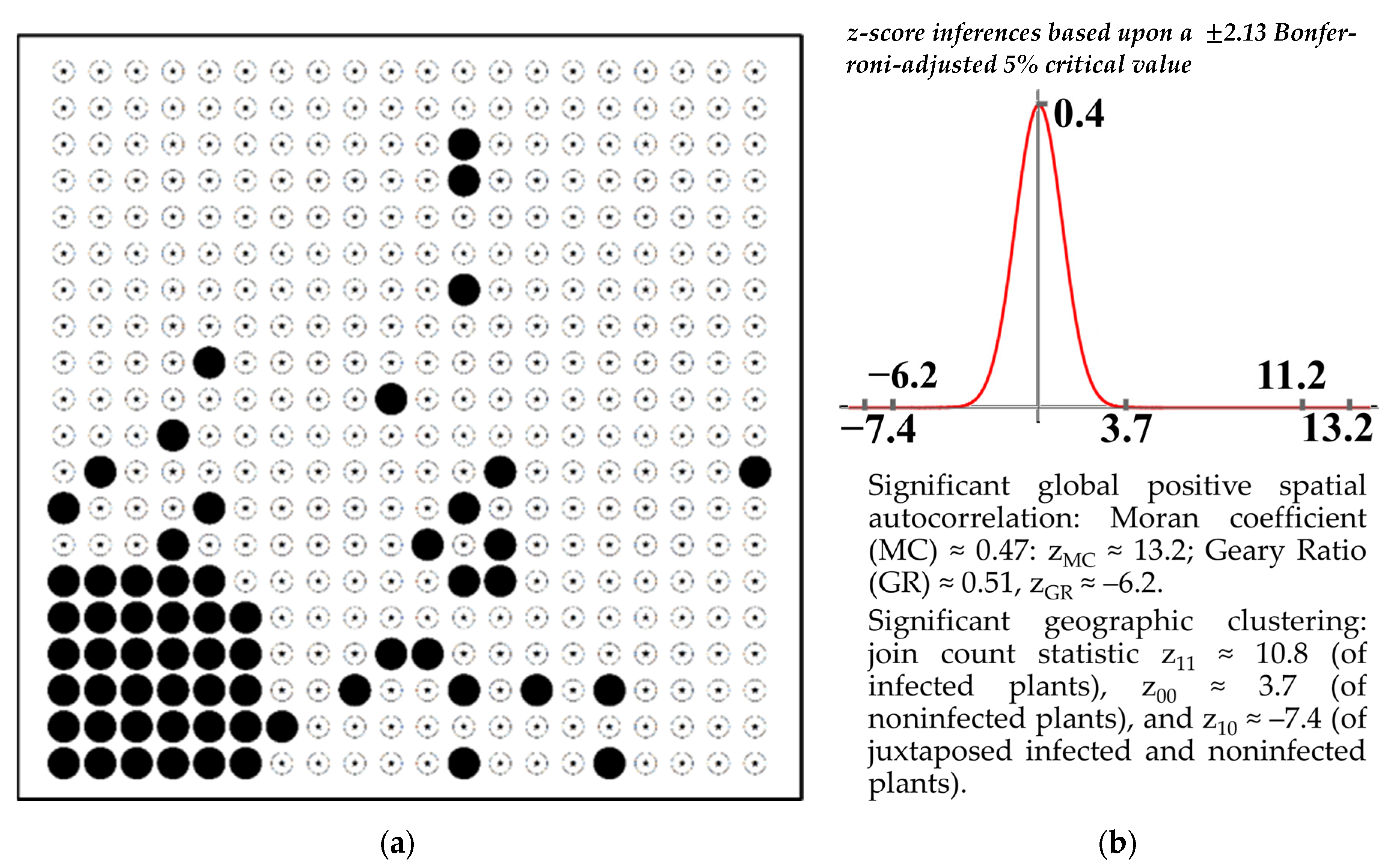
Graham [19], and Gumpertz et al. [20] furnish a 20 by 20 grid, superimposed upon an agricultural field plot, of geotagged Phytophthora root and crown rot disease incidence in bell pepper plant data measured with a binary 0–1 presence–absence Bernoulli response variable (see Figure 2); their analyses utilize an auto-logistic model, in keeping with Besag [21]. This section analyzes part of these geospatial data which display statistically significant moderate positive spatial autocorrelation. These specimen data contain 61 infected plants, yielding an empirical presence probability of 61/400 ≈ 0.1525 (i.e., the Bernoulli average sample probability that a response of one occurs). Their spatial correlation indices (see Figure 2), all of which are highly statistically significant (i.e., z-scores with critical region p-values near zero), suggest the description of a geographic distribution containing moderate positive spatial autocorrelation. The ensuing discussion examines the following three spatial statistical specifications of a Bernoulli regression equation depiction of these data, in turn: an auto-logistic (a spatial autoregressive form); a random effects (RE; a parametric mixture model form); and a Moran eigenvector spatial filter (MESF [22]; a standard GLM form). Each is a purely spatial autocorrelation descriptor, deliberately lacking any substantive covariates.
Figure 2.
Phytophthora root and crown rot disease incidence in bell pepper plants in an agricultural field; filled black circle and circumpunct symbols, respectively, denote infected and healthy plants. Left (a): the observed geographic distribution. Right (b): the spatial autocorrelation indices for Figure 2a; see ref. [23].
Hilbe [11] notes that extra-Bernoulli dispersion is not necessarily immediately apparent from a simple inspection of the customary Pearson or deviance dispersion statistics. Therefore, several preliminary alternative benchmark calculations now merit attention. The logistic regression intercept estimate (i.e., standard intercept-only GLM output), ignoring any latent spatial dependency component for the bell pepper data, gives e−1.7151/(1 + e−1.7151) ≈ 0.1525 ≈ 61/400, implying = 5.5574. Meanwhile, replacing 0 with 1 10−16 and 1 by 1−1 × 10⁻¹⁶ in this dataset facilitates exploring the aforementioned beta-Bernoulli convergence. A beta regression for this approximation involving a very slight perturbation produces an estimated beta parameter sum of (α + αK) ≈ 0.0905 (see [24]), and hence = 0.0905/(5.5574 + 1) = 0.0138, confirming that both beta parameters for the diseased bell pepper data are very close to zero; more specifically, the estimated beta parameter duo is (0.0138, 0.0767), generating an extremely pronounced U-shaped distribution.
4.1. The Bernoulli Auto-Logistic Spatial Statistical Model
Besag [21] devises this nearly successful auto-model conceptualization. His most successful innovation is the auto-normal, which should not be a surprise given the historical success of normal curve theory (see [25]); his near success is the auto-binomial, and hence its special case of the auto-Bernoulli/logistic. At least one weakness of this latter formulation is the pronounced covariation between its intercept and spatial autoregression parameters [26], seriously complicating its interpretation. Another is that its joint distribution estimation entails numerically intensive Markov chain Monte Carlo (MCMC) techniques, not GLM algorithms. One outcome is that, in practice, pseudo-likelihood (a prefix from the Greek word meaning false or untrue; [27])—maximizing the product of n conditional densities—first proposed by Besag [28], has been preferred to MCMC estimation primarily because of the former’s computational simplicity (i.e., ease of implementation as well as an artificial likelihood profile concavity mimicking a likelihood function approximation), combined with its ability to provide good mean response parameter estimates, although not necessarily a sound inferential basis for them. This section summarizes selected pseudo-likelihood findings because its focus is on the predicted probabilities computed with parameter estimates, not inferences about these estimates themselves.
The auto-logistic equation may be written as follows (e.g., [29]):
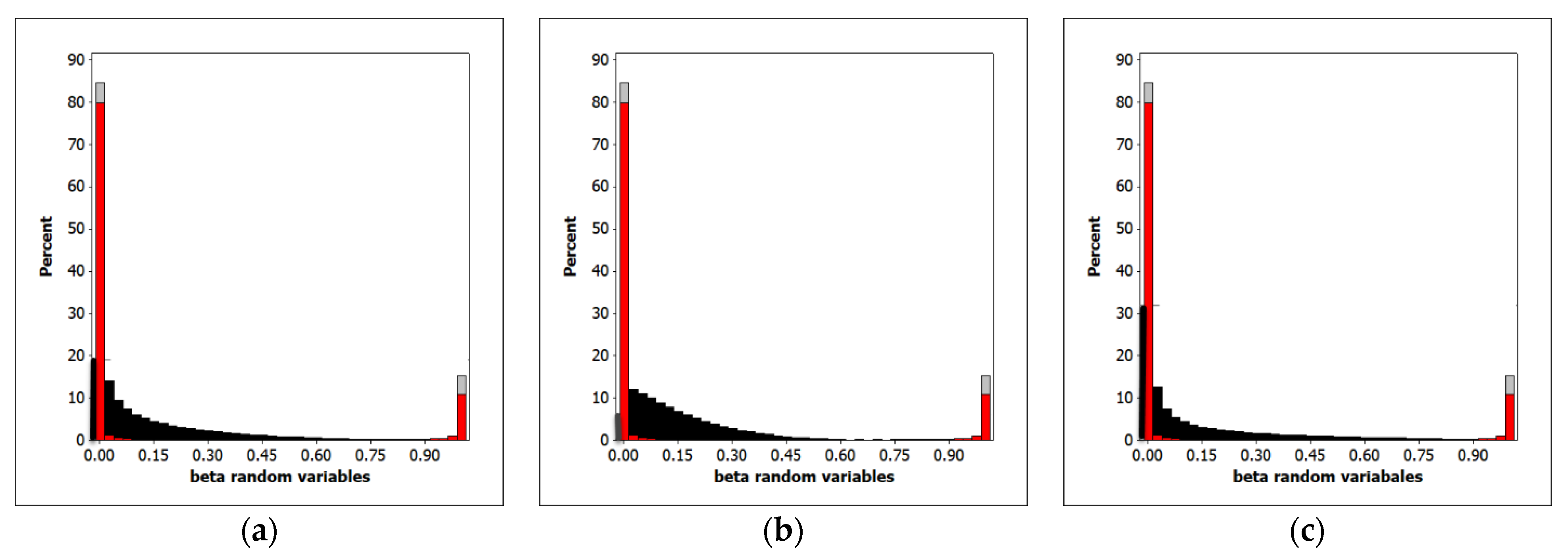
where Pr denotes probability, wij is the (i,j)th cell entry in an n-by-n spatial weights matrix capturing the locational configuration of geotagged observations (e.g., the regular square lattice structure underlying Figure 2a, here with a rook adjacency definition attached to it)—wij > 0 if locations i and j are juxtaposed (i.e., their invisible regular square tessellation mesh cells share a non-zero length common boundary), and 0 otherwise—and ρ denotes the spatial autocorrelation parameter. Figure 3c portrays the map pattern focus of the spatial lag term: as the Moran coefficient and two positive spatial autocorrelation join count statistics highlight, the coterminous patches of infected and noninfected plants tend to increase the value of ρ, whereas, as the Geary ratio and third join count statistic underscore, the boundaries of these patches coupled with isolated single and relatively very small infected plant concentrations tend to decrease the value of ρ. Pseudo-likelihood estimates employing the diseased bell pepper plant data are: intercept ≈ −2.9346 and ≈ 1.2773, using positive spatial weights matrix entries of 1. The aforementioned intercept autoregressive parameter interpretation difficulty (also [30]) is evident in this output, e.g., the intercept estimates changes from −1.7151 to −2.9346), and > 1. Meanwhile, the accompanying pseudo-R2 implication is that spatial autocorrelation accounts for roughly 40% of the geographic variation in diseased plants across the agricultural field plot under study. The new simplified-parameters beta regression (K + 1) is 3.4368. Substituting these sundry computations into portions of Conjecture 1 reveals the following sequence (see Figure 4a for their graphic portrayals),
Clearly these binary data have more variability than allowed by the conventional Bernoulli distributional assumptions. Hilbe’s implicit over-dispersion accounting for this beta-Bernoulli variance inflation is the difference between 0.22092, for the spatially autocorrelated data, and 0.17052, for their iid counterpart. Replacing these typically invisible or glossed-over probabilities with the observed Bernoulli 0–1 values automatically relegates the binary data variance to 0.36002, masking these two hitherto hidden quantities.
4.2. The Bernoulli RE Spatial Statistical Model
Whereas the auto-normal is a complete success, in both its simultaneous (i.e., SAR) and conditional autoregressive (i.e., CAR) renderings, and the auto-logistic and binomial are partial successes, perhaps the most consequential Besag spatial dependency model failure is the widely craved auto-Poisson [19], which is unable to characterize the inescapable preponderance of positive spatial autocorrelation situations. Although this breakdown feature extends to others of his auto-models (e.g., the auto-gamma, and the auto-negative binomial his work motivated), with some of his peer spatial statisticians concocting awkward remedies for its shortcomings (e.g., [31]) in order to salvage it, Besag and certain of his colleagues [32] turned their attention to clustered statistical models that incorporate RE—a notion whose basic idea Fisher [33] first articulated (p. 127, ref. [4] reports that Eisenhart [34] invented this exact phrasing)—to account for the observation correlation-induced clustering structure in, for example, binary data (i.e., a clustered Bernoulli random variable [35]), thus allowing for more accurate estimation and inference when dealing with correlated observations. Accordingly, they replaced his initial auto-models with RE Gaussian mixture models—frequentist probability models, for example, describing data containing repeated measures invariant unobserved heterogeneity, uncorrelated with their mean response regression covariates, if any, in which density/mass function parameters are random variables (e.g., [36]). This paradigm shift was possible because Besag and his research associates could take advantage of remarkable computational methods and statistical software advances occurring during the 1970s and 1980s, (e.g., WinBUGS with its 1989 debut; [37]), enabling estimation and interpretation of RE models. He also retained his successful auto-normal model in his new creation, defining his synthetic RE variate in terms of a CAR spatial dependency structure. As such, he introduced a two-component RE term to handle spatial autocorrelation effects: spatially structured (SSRE) accounting for geographically patterned (i.e., spatial autocorrelation induced), and spatially unstructured (SURE) accounting for aspatial stochastic (e.g., white noise), variation. SSRE estimation involves the intrinsic CAR (i.e., ICAR; see [30]) formulation implementation that facilitates simplifying MCMC estimation; unfortunately, its joint RE density is improper. Although a traditional CAR model captures rather weak spatial autocorrelation, its embedding in a model parameter enhances it so that it is able to account for marked spatial autocorrelation, when required. In addition, Besag’s RE approach avoids a need for repeated measures by employing a prior distribution within a Bayesian analysis context to input the mandatory additional information necessary to estimate a RE term. Fortunately, this more recent fabrication by Besag extends spatial statistical models handling spatial autocorrelation to any random variable harboring a regression version, not just the handful of statistical distributions appearing in the auto-model literature.
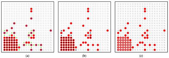
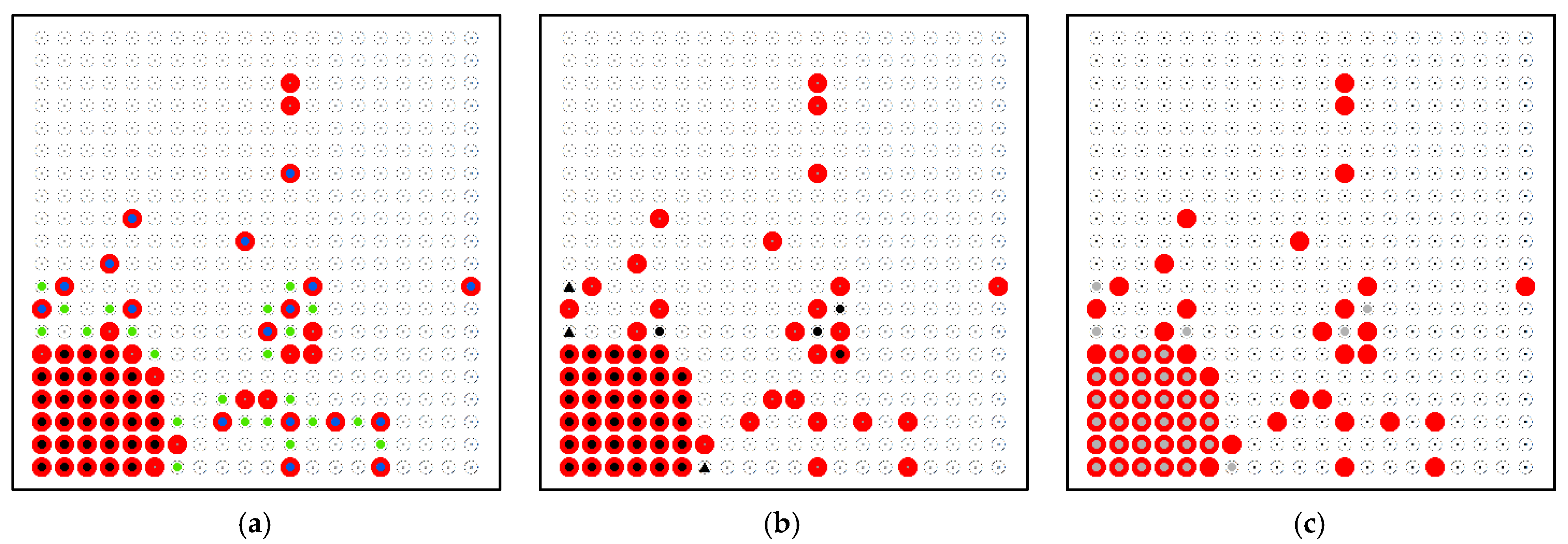
Figure 3.
Local indices of spatial autocorrelation demarcated geographic clusters; solid red circles and circumpunct symbols, respectively, denote infected plants and non-statistically significant results. Left (a): LISA [38]; solid black, blue, and green filled embedded circles, respectively, denote high-high (HH), high-low (HL), and low-low (LL) concentrations. Center (b): Getis–Ord statistic [39]; solid black filled embedded circles and triangles, respectively, denote 99%, and 90% statistically significant hot spots. Right (c): the intersection of Figure 3a,b maps: solid gray filled embedded circles denote dually marked plants.
The ICAR RE Bayesian mathematical expressions may be written as follows [40]:
where si is a RE value for pepper plant i, with s denoting its n-by-1 vector and s-i denoting the spatial lag term wis for spatial weights matrix W row vector i (indicating a conditional distribution of value si on its designated nearest neighbors), μi is the mean of first-order spatial neighboring RE values for pepper plant i, is the RE variance, and ni is the number of first-order neighbors for pepper plant i. Unfortunately, Bayesian parameter estimation for the ICAR-based hierarchical structure (2) with the WinBUGS platform entails MCMC chains that suffer from numerous repeated failures in their numerical convergence across a wide range of initial parameter values. Therefore, WinBUGS was replaced with the Integrated Nested Laplace Approximation (INLA) R package implementation that employs the Laplace approximation [41] to Bayesian computations, a more robust approach that has been around since roughly 2009 (see [42,43]). INLA Bayesian estimates for the diseased bell pepper plants data are intercept ≈ −2.63 and an approximated ICAR RE with a mean of 0.001, a Shapiro–Wilk normality diagnostic statistic of 0.959 (p < 0.001), and a Moran coefficient of 0.80 and a Geary Ratio of 0.17 (i.e., strong positive spatial autocorrelation). Meanwhile, the accompanying pseudo-R2 implication is that spatial autocorrelation accounts for roughly 53% of the geographic variation in diseased plants across the agricultural field plot under study. The new beta regression (K + 1) is 6.9547. Substituting these sundry computations into their corresponding parts of Conjecture 1 reveals the following sequence (see Figure 4b for their graphic portrayals),
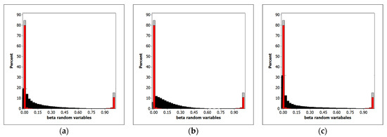
Figure 4.
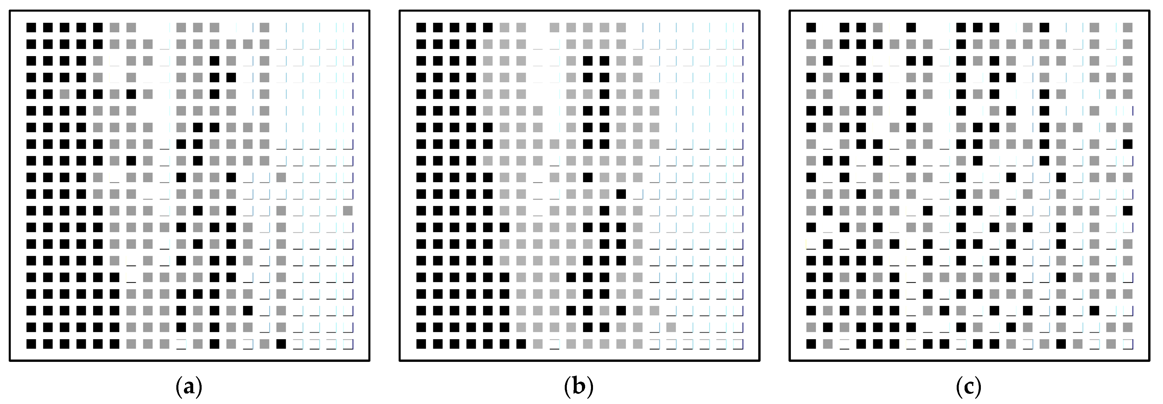
Comparative variance inflation histogram overlays (n = 2000; systematic Blom [44] defined CDF samples): iid beta, asymptotic beta, and beta-Bernoulli plots, respectively, denoted by black, red, and gray filled rectangles; asymptotic beta integrals yield 0.8481 for interval [0, 0.5] and 0.1519 for interval [0.5, 1]. Left (a): auto-logistic-based output. Middle (b): RE-based output. Right (c): MESF-based output.
Once more, these binary data obviously have more variability than allowed by the iid Bernoulli distributional assumptions. Hilbe’s implicit over-dispersion accounting for this beta-Bernoulli variance inflation is the difference between 0.14222, for the spatially autocorrelated data, and 0.12752, for their iid counterpart. As mentioned previously, replacing these typically invisible or glossed-over probabilities with the observed Bernoulli 0–1 values automatically relegates the binary data variance to 0.36002, masking these two hitherto hidden quantities.
Because this analysis exploits posited priors, (an inferior source of ancillary information by itself because it can be susceptible to overfitting of residuals (also see [45])), rather than repeated space-time data, (a reliable source when facts and figures are available for a sufficient number of time periods), its RE estimate apparently suffers, as a visual contrasting of Figure 2a and Figure 5a discloses. An SSRE component (Figure 5b) aligning with a lower-left- to upper-right-hand trend, rather than simply a left-to-right-hand horizontally oriented trend, would be more representative of the geographic distribution of the detected bell pepper disease infections.
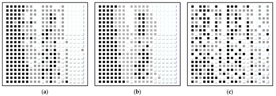
Figure 5.
INLA RE output; tertile maps in which white, gray, and black, respectively, denote relatively low, moderate, and high synthetic values. Left (a): the INLA composite RE (rendering a SAR autocorrelation parameter of ≈ 0.899). Middle (b): the SSRE component (Moran coefficient ≈ 0.90; Geary Ratio ≈ 0.06). Right (c): the SURE component (Moran coefficient ≈ −0.11; Geary Ratio ≈ 1.10).
4.3. The Bernoulli MESF Spatial Statistical Model
MESF offers a third feasible and effective methodological treatment of spatially autocorrelated Bernoulli random variables (e.g., [46]; also see [47]). It employs judiciously selected eigenvectors from a doubly centered spatial weights matrix—the principal matrix algebraic expression in the numerator of a Moran coefficient—as covariates to account for spatial autocorrelation latent in a geographic distribution. The orthogonality and uncorrelatedness of these vectors coupled with a multiple testing adjustment (also see [48]) bolster the trustworthiness of this stepwise regression analytic approach. Tiefelsdorf and Griffith [49] show that this transformation is a dimension reduction/simplification alternative to the auto-regressive spatial lag term: both utilize the same spatial weights matrix, but MESF dismisses eigenvectors latent in this matrix that are not strongly correlated with the given binary response variable, and hence introduce corrupting noise into a conventional auto-logistic analysis.
The auto-logistic equation here may be rewritten/approximated as follows (e.g., [46]):
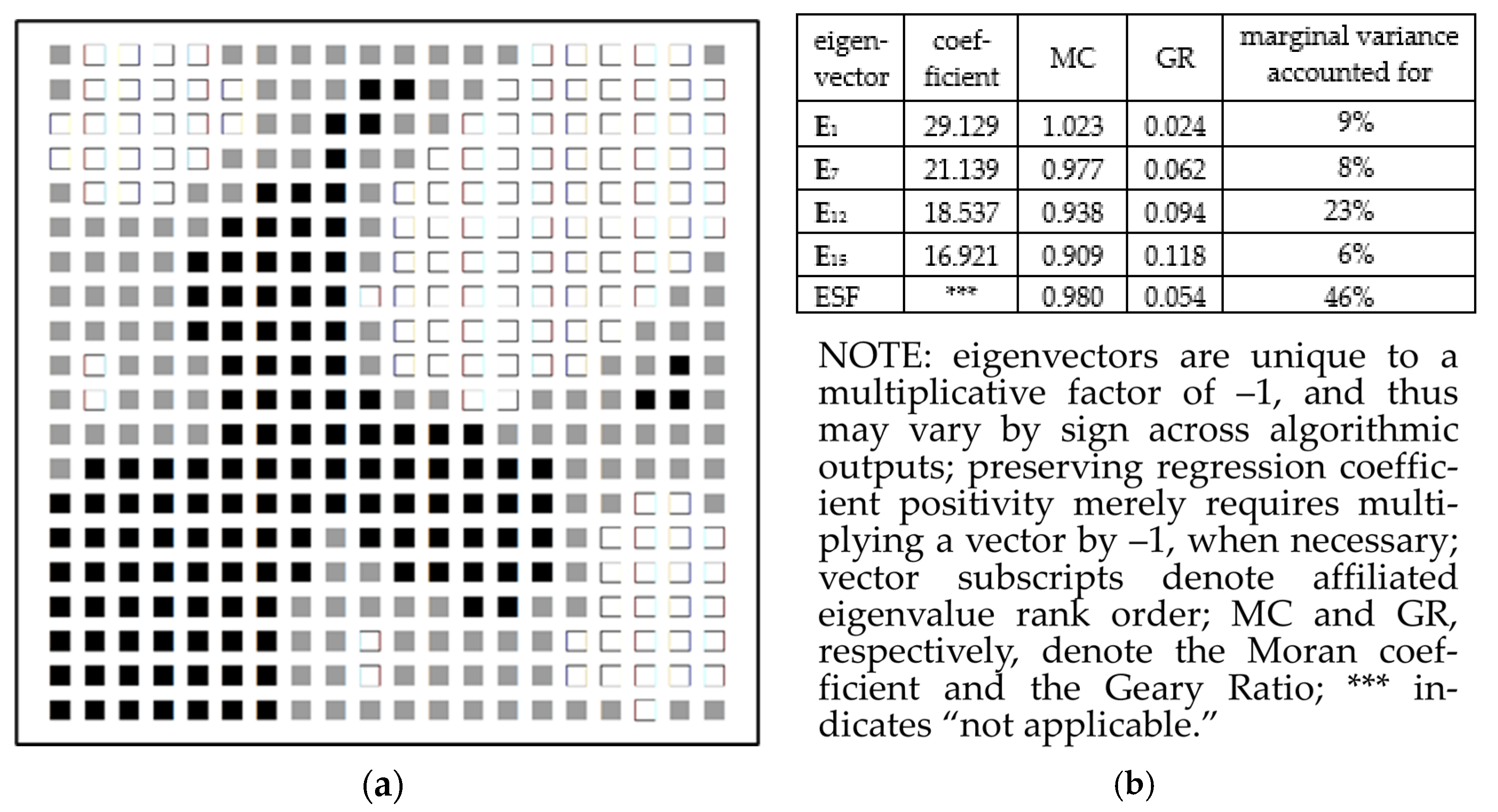
where denotes an eigenvector spatial filter (ESF)—a weighted linear combination of judiciously selected, doubly centered spatial weights matrix eigenvectors. Stepwise logistic regression for this pepper plant, disease incidence data analysis involves a candidate set of 123 positive and 124 negative, (from a total of 399), spatial autocorrelation eigenvectors using a Moran coefficient threshold of 0.25. Executing this GLM procedure extracts four positive spatial autocorrelation eigenvectors that render an ESF (see Figure 6; also, visually compare it with Figure 2) whose accompanying pseudo-R2 implication is that spatial autocorrelation accounts for roughly 46% of the geographic variation in diseased plants across the agricultural field plot under study. This slight increase vis-à-vis the preceding auto-logistic specification is attributable to a reduction in covariate noise achieved by replacing a spatial lag with an ESF. Ordinary GLM estimates for the diseased bell pepper plant data are intercept ≈ −2.6142, which again is comparable to the preceding auto-logistic result. The ESF Moran coefficient, which is easier to immediately interpret than the auto-logistic value, suggests very strong positive spatial autocorrelation. The aforementioned auto-logistic interpretation difficulty seems to persist in this output (e.g., the intercept estimate now changes from −1.7151 to −2.6142); this result alludes to the issue Caragea and Kaiser [30] address, concerning geographic distributions over regular square lattices of observed Bernoulli response variables representing presence/absence. Meanwhile, the new beta regression (K + 1) is 2.0073. Substituting these sundry computations into their matching Conjecture 1 parts reveals the following sequence (see Figure 4c for their graphic portrayals):
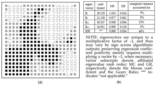
Figure 6.
Selected MESF analysis output. Left (a): a tertile map of the empirical four-vector constructed ESF; white, gray, and black, respectively, denote relatively low (i.e., negative; −4.9 to −0.7), moderate (i.e., near zero; −0.7 to 0.6), and high (i.e., positive; 0.6 to 7.8) regression coefficient weighted linear combination values. Right (b): certain ESF eigenvector statistics.
Yet again, these binary data clearly have more variability than allowed by the original Bernoulli distributional assumptions. Hilbe’s implicit over-dispersion accounting for this beta-Bernoulli variance inflation is the difference between 0.23072 for the spatially autocorrelated data, and 0.20732 for their iid counterpart. As before, replacing these typically invisible or glossed-over probabilities with the observed Bernoulli 0–1 values automatically relegates the binary data variance to 0.36002, masking these two hitherto hidden quantities.
5. Concluding Comments
The overarching objective of this paper is to extend the logistic regression comprehension promoted by Hilbe [11] by providing, for the first time, a detailed explanation of the meaning of his implicit extra-dispersion notion for Bernoulli response variables. For example, the spatial autocorrelation infused variance inflation that creates extra binomial variation, in turn generating an increasingly conspicuous U-shape distributed beta random variable as its probability density function increasingly bifurcates to approach, in the limit, a Bernoulli mass function on the integer points 0 and 1 of the support interval [0, 1] that ultimately, a(n) (ir)rational-to-integer numbers rounding routine masks. This definition builds upon well-known and long-established variance formulae for beta, beta-binomial, and Bernoulli random variables, as well as the already known asymptotic convergence of a beta-binomial on a Bernoulli distribution. One novel contribution is a cogent demonstration that a spatially autocorrelated Bernoulli is not necessarily a quasi-binomial distribution, countering another segment of the conventional wisdom circulating about this subject. In addition, summarized illustrations of various Bernoulli over-dispersion assessments contained in this paper employ a readily accessible and published-about bell pepper plant disease dataset. These empirical examples quantify spatial autocorrelation and its variance effects, and then differentiate between its induced variance inflation and the masking of this over-dispersion by shifting to a Bernoulli distribution substitution. The three model specifications for completing this decomposition are: Besag’s auto-logistic, Besag’s ICAR RE (a la INLA approximation), and the more novel MESF GLM. Table 1 tabulates the Bernoulli rounded-to-integer outcomes of Equations (1)–(3); all three specifications yield comparable results, with the RE specification producing the poorest and the MESF producing the best of these triplet sets. As an aside, these conclusions generalize to other correlated data sources, such as time series sequence structuring.

Table 1.
Rounded-off predicted probabilities: from a beta to a Bernoulli random variable.
Although some conceptualizations presented in this paper are reminiscent of sundry pieces of the existing literature, with such arguments as the beta convergence on a Bernoulli recognized as not being surprising to scholars in the subfield dedicated to logistic regression (who often openly nurture an awareness of it), this appears to be the first systematic writing explicitly and comprehensively detailing and expanding upon it in a single organized narrative. Figure 1 and Figure 2 serve as effective visualizations of this notion. Its spatially autocorrelated Bernoulli specification not definitively being a quasi-binomial distribution also is an interesting discovery. Figure 3 and Figure 4 furnish illuminating portrayals of this empirical context, emphasizing the role of map pattern coupled with variance inflation attributable to spatial autocorrelation. Figure 5 and Figure 6 take it one step further, illustrating how a specimen geospatial dataset relates to both the frequentist and the Bayesian perspectives about this theme. In the tradition of remote sensing classification analysis employing a multinomial distribution (e.g., the kappa index), Table 1 provides a confusion matrix-type cross-tabulation to exemplify prominent spatial autocorrelation impacts on 2-point Bernoulli random variables. Therefore, the major contribution this paper makes is a better clarification and deeper understanding of logistic regression extra-Bernoulli variation, particularly that attributable to correlated data.
Funding
This research received no external funding.
Institutional Review Board Statement
Not applicable.
Informed Consent Statement
Not applicable.
Data Availability Statement
The data analyzed in this article are readily accessible from their free publicly available cited sources.
Acknowledgments
This paper is a tribute to Joseph M. Hilbe (1944–2017), co-author of [50], in recognition of his exceptional contributions to logistic regression theory and practice. The author is an Ashbel Smith Professor of Geospatial Information Sciences.
Conflicts of Interest
The author declares no conflicts of interest.
References
- Poisson, S.-D. Recherches sur la Probabilitƺé des Jugements en Matiére Criminelle et en Matiére Civile Précédées des Régles Générales du Calcul des Probabilités; Bachelier: Paris, France, 1837. [Google Scholar]
- Cramer, J. The Origins of Logistic Regression; Discussion Paper No. 2002-119/4; Tinbergen Institute: Amsterdam, The Netherlands, 2002. [Google Scholar] [CrossRef]
- Verhulst, P.-F. La loi d’Accroissement de la population. Nou-Veaux Mem. L’academie R. Des Sci. Belles-Lett. Brux. 1845, 18, 1–59. [Google Scholar]
- David, H. First (?) occurrence of common terms in mathematical statistics. Am. Stat. 1995, 49, 121–133. [Google Scholar]
- Berkson, J. Application of the logistic function to bio-assay. J. Am. Stat. Assoc. 1944, 39, 357–365. [Google Scholar]
- Bayes, T. An essay towards solving a problem in the doctrine of chances. Philos. Trans. R. Soc. Lond. 1763, 53, 370–418. [Google Scholar] [CrossRef]
- Skellam, J. A probability distribution derived from the binomial distribution by regarding the probability of success as variable between the sets of trials. J. R. Stat. Soc. B 1948, 10, 257–261. [Google Scholar] [CrossRef]
- Skrondal, A.; Rabe-Hesketh, S. Redundant overdispersion parameters in multilevel models for categorical responses. J. Educ. Behav. Stat. 2007, 32, 419–430. [Google Scholar] [CrossRef]
- Morrissey, M.; de Villemereuil, P.; Doligez, B.; Gimenez, O. Chapter 14: Bayesian approaches to the quantitative genetic analysis of natural populations. In Quantitative Genetics in the Wild; Charmantier, A., Garant, D., Kruuk, L., Eds.; Oxford University Press: Oxford, UK; New York, NY, USA, 2014; pp. 228–253. [Google Scholar]
- Dohoo, I.; Martin, W.; Stryhn, H. Chapter 16: Logistic Regression, Veterinary Epidemiology Research; VER Inc.: Charlottetown, PE, Canada, 2014; pp. 395–426. Available online: http://projects.upei.ca/ver/files/2022/08/VER_ch16.pdf (accessed on 10 February 2024).
- Hilbe, J. Can Binary Logistic Models Be Overdispersed? Unpublished Manuscript. 2013. Available online: http://www.highstat.com/Books/BGS/GLMGLMM/pdfs/HILBE-Can_binary_logistic_models_be_overdispersed2Jul2013.pdf (accessed on 30 November 2023).
- Feller, W. An Introduction to Probability Theory and Its Applications; Wiley: New York, NY, USA, 1971; Volume 2. [Google Scholar]
- Schonlau, M. Applied Statistical Learning: With Case Studies in Stata; Springer: Cham, Switzerland, 2023. [Google Scholar]
- Available online: https://math.stackexchange.com/questions/2905844/beta-distribution-with-parameters-alpha-beta-to-0-is-bernoulli-distribution (accessed on 25 February 2024).
- Siwale, I. A New Proof of Fisher’s Invariance Theorem; Technical Report No. RD-26-2015; Zenith Genetica Ltd.: London, UK, 1997; Available online: https://www.researchgate.net/publication/285928037_A_New_Proof_of_Fisher%27s_Invariance_Theorem (accessed on 10 February 2024).
- Mielke, P.W. Convenient Beta Distribution Likelihood Techniques for Describing and Comparing Meteorological Data. J. Appl. Meteorol. 1975, 14, 985–990. [Google Scholar] [CrossRef][Green Version]
- Wedderburn, R. Quasi-likelihood functions, generalized linear models, and the Gauss—Newton method. Biometrika 1974, 61, 439–447. [Google Scholar]
- Leach, J.; Aban, I.; Yi, N. Incorporating spatial structure into inclusion probabilities for Bayesian variable selection in generalized linear models with the spike-and-slab elastic net. J. Stat. Plan. Inference 2021, 217, 141–152. [Google Scholar] [CrossRef]
- Graham, J. Markov chain Monte Carlo methods for modeling the spatial pattern of disease spread in bell pepper. In Proceedings of the 8th Annual Conference on Applied Statistics in Agriculture, Manhattan, KS, USA, 28–30 April 1996; Milliken, G., Ed.; Department of Statistics, Kansas State University, New Prairie Press: Manhattan, KS, USA, 1996; pp. 91–108. [Google Scholar] [CrossRef]
- Gumpertz, M.; Graham, J.; Ristaino, J. Autologistic model of spatial pattern of Phytophthora epidemic in bell pepper: Effects of soil variables on disease presence. J. Agric. Biol. Environ. Stat. 1997, 2, 131–156. [Google Scholar] [CrossRef]
- Besag, J. Spatial interaction and the statistical analysis of lattice systems. J. R. Stat. Soc. Ser. B 1974, 36, 192–225. [Google Scholar] [CrossRef]
- Griffith, D. Spatial Autocorrelation and Spatial Filtering: Gaining Understanding through Theory and Scientific Visualization; Springer: Berlin, Germany, 2003. [Google Scholar]
- Griffith, D. The Moran Coefficient for non-normal data. J. Stat. Plan. Inference 2010, 140, 2980–2990. [Google Scholar] [CrossRef]
- Ferrari, S.; Cribari-Neto, F. Beta regression for modelling rates and proportions. J. Appl. Stat. 2004, 31, 799–815. [Google Scholar] [CrossRef]
- Lohnes, P.; Cooley, W. Chapter 7: Normal curve theory. In Introduction to Statistical Procedures: With Computer Exercises; Wiley: New York, NY, USA, 1968; pp. 107–125. [Google Scholar]
- Graham, J. Monte Carlo Markov Chain Likelihood Ratio Test and Wald Test for Binary Spatial Lattice Data; Technical Report; Department of Statistics, North Carolina State University: Raleigh, NC, USA, 1994. [Google Scholar]
- Strauss, D. The many faces of logistic regression. Am. Stat. 1992, 46, 321–327. [Google Scholar]
- Besag, J. Statistical analysis of non-lattice data. Statistician 1975, 24, 179. [Google Scholar] [CrossRef]
- Cressie, N. Statistics for Spatial Data; Wiley: New York, NY, USA, 1991. [Google Scholar]
- Caragea, P.C.; Kaiser, M.S. Autologistic models with interpretable parameters. J. Agric. Biol. Environ. Stat. 2009, 14, 281–300. [Google Scholar] [CrossRef]
- Kaiser, M.S.; Cressie, N. Modeling Poisson variables with positive spatial dependence. Stat. Probab. Lett. 1997, 35, 423–432. [Google Scholar] [CrossRef]
- Besag, J.; York, J.; Mollié, A. Bayesian image restoration, with two applications in spatial statistics. Ann. Inst. Stat. Math. 1991, 43, 1–20. [Google Scholar] [CrossRef]
- Fisher, R. The correlation between relatives on the supposition of Mendelian inheritance. Trans. R. Soc. Edinb. 1918, 52, 399–433. [Google Scholar] [CrossRef]
- Eisenhart, C. The Assumptions Underlying the Analysis of Variance. Biometrics 1947, 3, 1–21. [Google Scholar] [CrossRef]
- Kimpton, L.; Challenor, P.; Wynn, H. Modelling correlated Bernoulli data Part I: Theory and run lengths. arXiv 2022, arXiv:2211.16921. [Google Scholar] [CrossRef]
- Agresti, A.; Booth, J.; Hobert, J.; Caffo, B. Random-effects modeling of categorical response data. Sociol. Methodol. 2000, 30, 27–80. [Google Scholar] [CrossRef]
- Ntzoufras, I. Chapter 3: WinBUGS software: Introduction, setup, and basic analysis. In Bayesian Modeling Using WinBUGS; Wiley: New York, NY, USA, 2008; pp. 83–123. [Google Scholar]
- Anselin, L. The Local Indicators of Spatial Association—LISA. Geogr. Anal. 1995, 27, 93–115. [Google Scholar] [CrossRef]
- Ord, J.K.; Getis, A. Local spatial autocorrelation statistics: Distributional issues and an application. Geogr. Anal. 1995, 27, 286–306. [Google Scholar] [CrossRef]
- Besag, J.; Kooperberg, C. On conditional and intrinsic autoregressions. Biometrika 1995, 82, 733–746. [Google Scholar]
- Wang, G. Laplace approximation for conditional autoregressive models for spatial data of diseases. MethodsX 2022, 9, 101872. [Google Scholar] [CrossRef] [PubMed]
- Rue, H.; Riebler, A.; Sørbye, S.; Illian, J.; Simpson, D.; Lindgren, F. Bayesian computing with INLA: A review. Annu. Rev. Stat. Its Appl. 2017, 4, 395–421. [Google Scholar] [CrossRef]
- Bakka, H.; Rue, H.; Fuglstad, G.; Riebler, A.; Bolin, D.; Illian, J.; Krainski, E.; Simpson, D.; Lindgren, F. Spatial modeling with R-INLA: A review. Wiley Interdiscip. Rev. Comput. Stat. 2018, 10, e1443. [Google Scholar] [CrossRef]
- Blom, G. Statistical Estimates and Transformed Beta-Variables; Wiley: New York, NY, USA, 1958. [Google Scholar]
- Hodges, J.S.; Reich, B.J. Adding spatially-correlated errors can mess up the fixed effect you love. Am. Stat. 2010, 64, 325–334. [Google Scholar] [CrossRef]
- Griffith, D. A spatial filtering specification for the auto-logistic model. Environ. Plan. A 2004, 36, 1791–1811. [Google Scholar] [CrossRef]
- Borcard, D.; Legendre, P.; Avois-Jacquet, C.; Tuomisto, H. Dissecting the spatial structure of ecological data at multiple scales. Ecology 2004, 85, 1826–1832. [Google Scholar] [CrossRef]
- G’Sell, M.G.; Wager, S.; Chouldechova, A.; Tibshirani, R. Sequential selection procedures and false discovery rate control. J. R. Stat. Soc. 2015, 78, 423–444. [Google Scholar] [CrossRef]
- Tiefelsdorf, M.; Griffith, D. Semi-parametric filtering of spatial autocorrelation: The eigenvector approach. Environ. Plan. A 2007, 39, 1193–1221. [Google Scholar] [CrossRef]
- Hardin, J.; Hilbe, J. Generalized Linear Models and Extensions, 4th ed.; Stata Press: College Station, TX, USA, 2018. [Google Scholar]
Disclaimer/Publisher’s Note: The statements, opinions and data contained in all publications are solely those of the individual author(s) and contributor(s) and not of MDPI and/or the editor(s). MDPI and/or the editor(s) disclaim responsibility for any injury to people or property resulting from any ideas, methods, instructions or products referred to in the content. |
© 2024 by the author. Licensee MDPI, Basel, Switzerland. This article is an open access article distributed under the terms and conditions of the Creative Commons Attribution (CC BY) license (https://creativecommons.org/licenses/by/4.0/).


