A Note on Simultaneous Confidence Intervals for Direct, Indirect and Synthetic Estimators

Abstract

Direct, indirect and synthetic estimators have a long history in official statistics. While model-based or model-assisted approaches have become very popular, direct and indirect estimators remain the predominant standard and are therefore important tools in practice. This is mainly due to their simplicity, including low data requirements, assumptions and straightforward inference. With the increasing use of domain estimates in policy, the demands on these tools have also increased. Today, they are frequently used for comparative statistics. This requires appropriate tools for simultaneous inference. We study devices for constructing simultaneous confidence intervals and show that simple tools like the Bonferroni correction can easily fail. In contrast, uniform inference based on max-type statistics in combination with bootstrap methods, appropriate for finite populations, work reasonably well. We illustrate our methods with frequently applied estimators of totals and means.

1. Introduction

Nowadays, domain estimation is well recognised as an important sub-field in official statistics and survey methodology. The UN’s aspiration to leave nobody behind in its sustainable development goals has further boosted the interest in domain estimation, where “domains” may refer to any specified cluster or sub-population that could be of political or social interest. Governmental offices use those methods for the reallocation of resources and public programs [1]. Depending on the data availability, one may resort either to direct, indirect, model-assisted or even model-based methods to estimate or predict the parameters of interest; see the books [2,3]. Model-assisted or -based estimators are only interesting when appropriate auxiliary information is available. However, they rely on other data requirements, complex assumptions and methods, and, in the case of model misspecification, adverse effects on further inference can become substantial [4]. In contrast, design-based estimators are quite simple, work with weaker assumptions, do not necessarily need auxiliary information and can be assumed nearly design-unbiased [5,6]. The lack of auxiliary information—especially on the unit level—is a major problem in many cases and countries. Further problems arise when methods are not adapted to the inclusion of sampling weights. Even for model-based methodology, direct estimates are essential to start building and validating the models [1]. In sum, direct and indirect estimators remain useful tools in official statistics.

With the growing number of methods for estimating domain parameters, their use for decision making is growing too, quite frequently for comparative statistics over domains or even over small areas; c.f. [7]. Different authors like those of [8] critically observed that the topic of ensemble properties has been largely overlooked. Certainly, if one only wants to compare two domains, then a t-test is one of the obvious options, but often practitioners compare more than two domains simultaneously. Multiple comparison is a rather broad field in statistics [9]; in this article, we concentrate on simultaneous confidence intervals (SCIs) due to their easy interpretation and convenient handling. In a parametric unbiased context, this is an equivalent problem to simultaneous testing, though in practice those tests are often applied sequentially, which allows for more sophisticated modifications to control the family-wise error rate [10]. Recently, refs. [11,12] introduced different tools for simultaneous inference in the model-based small area estimation context, i.e., for estimators based on linear and generalized linear mixed models. For design-based estimators, we could not find any similar study; this paper is a contribution to fill this gap.

Some questions arise: Can we not simply apply the Bonferroni or the Šidák methods? One may also question if such an inference is practicable since for an increasing number of domains those intervals become very large. We will see that the first question (regarding the Bonferroni method) must be answered negatively, whereas the second is more involved. We believe that it is not too strong of a counterargument, as in practice one could conduct such comparisons on subsets of all domains. In contrast, conducting multiple comparison with tools made for individual analyses is definitely inappropriate. Even for a small set of domains, too-simple methods fail in delivering an appropriate joint coverage of the estimators.

Note that the considered problem is not related to the one faced in small area estimation based on mixed effects models, c.f. [13,14], regarding conditional versus unconditional inference. Both emphasise the problem that the typically reported coverage probabilities refer to the average over space and/or time without conditioning on the domains. When one repeatedly constructs some confidence intervals for the same set of domains, these can have 100% coverage for several domains and zero coverage for others. We do not face this problem because we only consider conditionally unbiased direct, indirect and synthetic estimators. This is just another advantage of the here-considered methods. The practical problem we refer to is equivalent to that of demanding uniform inference over a set of domains.

We first define SCIs and propose three practical methods for constructing them. Afterwards, we revisit the direct and indirect estimators for linear domain parameters, namely, totals and averages. Section 4 compares these methods when applied to those estimators. This is conducted for both simple and complex sampling designs and weights. Section 5 illustrates the use and performance of our methods using a data example in which we estimate total tax incomes for different domains in Belgium. Section 6 concludes this paper. More details on estimators, notation and simulations are deferred to our Supplementary Materials.

2. Simultaneous Confidence Intervals for Domains

For domain parameters ${\theta }_d$, $d=1,\dots ,D$, a simultaneous confidence interval ${\mathcal{I}}_{1-\alpha }$ at a fixed error level $0<\alpha <1$ forms a rectangular region that covers the set of parameters ${\theta }_d$ for all d of some finite collection $\mathcal{D}$ of D domains, with a probability of at least $1-\alpha$, i.e.,

$$\mathbb{P}\left({\mathcal{I}}_{1-\alpha }\ni {\theta }_d,\forall d\in \mathcal{D}\right)\ge 1-\alpha .$$

(1)

An SCI can be understood as the Cartesian product of D individual confidence intervals such that

$${\mathcal{I}}_{1-\alpha }=\underset{d\in \mathcal{D}}{\times }{\mathcal{I}}_{d;1-{\alpha }_d}\mathrm{with}{\mathcal{I}}_{d;1-{\alpha }_d}\left\{{\widehat{\theta }}_d\pm c_{1-{\alpha }_d/2}{\widehat{\sigma }}_d\right\},d=1,\dots ,D,$$

(2)

where $c_{1-{\alpha }_d}$ are suitable critical values and ${\widehat{\sigma }}_d$ consistent estimates of the standard deviation of ${\widehat{\theta }}_d$. For many of the direct and indirect estimators, standard errors can be estimated relatively easily. It is more challenging to find $c_{1-{\alpha }_d}$ such that Equation (1) holds. These ${\alpha }_d$ could be different from each other, but for practical reasons one would set them all to be equal, ${\alpha }_d={\alpha }^{\prime },\forall d$.

Obvious devices are the Bonferroni correction, the Šidák correction and the max-type statistic typically used for uniform inference. The Bonferroni correction can be applied by setting the individual levels to ${\alpha }^{\prime }=\alpha /D$ and choosing for $c_{1-{\alpha }^{\prime }/2}$ the $1-{\alpha }^{\prime }/2$ quantile of the student distribution with $n-D$ degrees of freedom, with n indicating sample size. (One may argue that one should take different critical values for each domain based on a $t_{n_d-1}$ distribution. At the same time, the approximation of the degrees of freedom is arguable since we are working with design-based estimators which include the use of potentially complex sampling weights. We will see in the simulations, however, that the Bonferroni approach will not even work in the simplest sampling design case.) Ref. [15] derived SCIs for arbitrary linear combinations of normally distributed means. Later on, this was taken as a justification to do the same for other estimators that are asymptotically normal. Ref. [16] proposed ${\alpha }^{\prime }=1-{(1-\alpha )}^{1/D}$ but suggested to otherwise use the same procedure. He showed that this correction can increase the multiple power uniformly.

The third approach considers the (relatively) largest deviation for all considered estimates, i.e., a max-type statistic. Refs. [11,12] applied this idea to small area estimation and introduced bootstrap procedures to approximate the distribution of the resulting pivotal statistic. In our case, such a max-type statistic is

$$S_0=\underset{d\in \mathcal{D}}{max}|S_{0;d}|,\mathrm{where}{S}_{0;d}:=\frac{{\widehat{\theta }}_d-{\theta }_d}{{\widehat{\sigma }}_d}.$$

(3)

It is recommend to use a resampling distribution of $S_0$ to approximate critical values. While the above-mentioned authors used model-based parametric bootstrap, we do not have a model. Furthermore, we need a bootstrap procedure that works for finite populations. There exist many proposals for those problems; in our simulations, we follow the recommendations of [17]. See also our Supplementary Materials for details, procedures and further references.

We close this section with a remark: there exist many modifications of the Bonferroni correction. Most of these were made in order to better control for potential correlations between testing or estimation problems. This can increase the power of a multiple test or decrease the length of SCIs. In our simulations, the estimates are uncorrelated such that those modifications are not of interest for our study—which is not necessarily the case in practice. As we will see that, in our context, the problem with Bonferroni is not an over- but a serious undercoverage, those modifications are therefore expected to produce worse results. In practice, the distributions of some domain parameter estimates have larger tails than the asymptotic distribution suggests. Consequently, the problem is less the proposed correction as it is finding an appropriate $c_{1-{\alpha }^{\prime }/2}$ that could be useful in practice.

3. Considered Direct and Indirect Estimators

One of the main benefits of direct methods is that they lead to design-consistent estimation and nearly design-unbiased estimators [18]. We concentrate on two popular estimators, the Horvitz–Thompson [19] (H-T) and the direct generalized regression estimator (GREG) [20] to estimate the total $Y_d:={\sum }_{k\in U_d}{y}_k$. One could alternatively consider any linear function of the $y_k$, but for the sake of presentation we concentrate on the simplest case. This is because (a) for our simulations we need to consider a specific one, (b) together with the domain mean, the total is one of the most frequently demanded parameters and (c) we will see that even for the simplest case, the considered standard devices do not work. In the following, the $Y_d$ are our parameters of interest, our ${\theta }_d$. The quantities ${\pi }_k,{\pi }_{k\ell }$ denote, respectively, the first-order inclusion probability of unit k and the second-order one of units k and ℓ. ${\Delta }_{k\ell }$ is the covariance between the inclusion probabilities of units k and ℓ within the same sample. Then, the H-T estimator is

$${\widehat{Y}}_d^{ht}:=\sum _{k\in s_d}\frac{y_k}{{\pi }_k},$$

(4)

and similarly ${\widehat{\overline{Y}}}_d^{ht}=N_d^{-1}{\widehat{Y}}_d^{ht}$ for the mean with $N_d$ the domain size.

As said, when auxiliary variables $x_k\in {\mathbb{R}}^p,p\ge 1$ are available and their totals are known, then domain-level linear mixed models become more and more popular in practice. The more traditional ancestor is the direct-GREG approach, an estimator assisted by a standard linear regression model with errors ${ϵ}_{kd}$, i.e.,

$$y_{kd}=x_{kd}^{\top }{\beta }_d+{ϵ}_{kd},\mathrm{Var}\left({ϵ}_{kd}\right)={\sigma }_{kd}^2,$$

(5)

where ${\beta }_d$ is a parameter vector associated with domain $U_d$, typically estimated by

$${\widehat{\beta }}_d={\left(\sum _{k\in s_d}\frac{x_k{x}_k^{\top }}{{\pi }_k}\right)}^{-1}\left(\sum _{k\in s_d}\frac{x_k{y}_k}{{\pi }_k}\right).$$

(6)

The direct-GREG is

$${\widehat{Y}}_d^{dgreg}:=\sum _{k\in U_d}{\widehat{y}}_k+\sum _{k\in s_d}\frac{e_k}{{\pi }_k}={\widehat{Y}}_d^{ht}+{(X_d-{\widehat{X}}_d^{ht})}^{\top }{\widehat{\beta }}_d,$$

(7)

where $X_d$ is the vector of true domain totals for each auxiliary variable, $e_k=y_k-{\widehat{y}}_k$ and ${\widehat{X}}_d^{ht}$ is its Horvitz–Thompson estimator.

Indirect estimators borrow strength from domains or clusters that are different from the domains of interest [21]. Therefore, we introduce here the notion of groups. These are subsets $U_g,g=1,\dots ,G$, different from the domains and not necessarily of interest, that partition the population, i.e., ${\bigcup }_{g=1}^G{U}_g=U,\mathrm{with}{U}_g\bigcap U_{g^{\prime }}=Ø\mathrm{for}g\ne g^{\prime }$. Typically, G is small. An estimator of a group’s mean ${\overline{Y}}_g$ is given by

$${\widehat{\overline{Y}}}_g:=\frac{1}{{\widehat{N}}_g^{ht}}\sum _{k\in s_g}\frac{y_k}{{\pi }_k}=\frac{{\widehat{Y}}_g^{ht}}{{\widehat{N}}_g^{ht}}\mathrm{where}{\widehat{N}}_g^{ht}:=\sum _{k\in s_g}\frac{1}{{\pi }_k},$$

(8)

also known as the Hajek estimator [22]. The synthetic estimator (Syn) for the total in domain d is

$${\widehat{Y}}_d^{synth}:=\sum _{g=1}^G{N}_{dg}{\widehat{\overline{Y}}}_g,$$

(9)

where $N_{dg}$ are the crossed population sizes between domain d and group g.

A modification of the synthetic estimator is its post-stratified version (P-S). Instead of using the group’s mean, one uses the means in subsets $U_{dg}=U_d\bigcap U_g$,

$${\widehat{Y}}_d^{psts}:=\sum _{g=1}^G{N}_{dg}{\widehat{\overline{Y}}}_{dg},\mathrm{where}{\widehat{\overline{Y}}}_{dg}:=\frac{1}{{\widehat{N}}_{dg}^{ht}}\sum _{k\in s_{dg}}\frac{y_k}{{\pi }_k}\mathrm{with}{\widehat{N}}_{dg}^{ht}:=\sum _{k\in s_{dg}}\frac{1}{{\pi }_k}.$$

(10)

This estimator is generally unbiased [3] and performs better than the basic synthetic estimator when $y_k$ has a large variation within groups.

The indirect-GREG estimator (I-GREG) for the total can also be considered as an indirect estimator under regression $y_k=x_k^{\top }\beta +{ϵ}_k$, i.e., with a common parameter vector $\beta$ for the population, instead of one for each domain [23]. Similar to the direct-GREG, it is defined by

$$\widehat{\beta }={\left(\sum _{k\in s}\frac{x_k{x}_k^{\top }}{{\pi }_k}\right)}^{-1}\sum _{k\in s}\frac{x_k{y}_k}{{\pi }_k},$$

and the I-GREG estimator of the total is for ${\widehat{y}}_k=x_k^{\top }\widehat{\beta }$ and $e_k=y_k-{\widehat{y}}_k$ given as

$${\widehat{Y}}_d^{igreg}:=\sum _{k\in U_d}{\widehat{y}}_k+\sum _{k\in s_d}\frac{e_k}{{\pi }_k}={\widehat{Y}}_d^{ht}+{\left(X_d-\widehat{X_d^{ht}}\right)}^{\top }\widehat{\beta }=\sum _{k\in s}\frac{g_{dk}{y}_k}{{\pi }_k},$$

(11)

where $g_{dk}:=I_{dk}+{(X_d^{ht}-{\widehat{X}}_d^{ht})}^{\top }{({\sum }_{k\in s}{x}_k{x}_k^{\top }/{\mathbf{\pi }}_k)}^{-1}$.

If $N_d$ is known, Equation (11) can be simplified [23] to

$${\widehat{Y}}_d^{igreg}:=\sum _{k\in U_d}{\widehat{y}}_k+\frac{N_d}{{\widehat{N}}_d^{ht}}\sum _{k\in s_d}\frac{e_k}{{\pi }_k}.$$

(12)

For more details about these estimators, see our Supplementary Materials and [3,20,23].

4. Simulation Studies

The aim of our simulation study is to better understand the performance of the above methods. Specifically, we compare the actual coverage probabilities of different SCIs of all combinations of estimators and methods to construct SCIs. As said, here, we consider the estimation of domain totals or functions of them. To keep it simple, we perform this first for samples of small and moderate size and then consider what happens to the best combinations when sample sizes increase a bit.

4.1. Simulation Designs

As we included GREG estimators in our study, we need to use a hierarchical model for generating the data for populations U. We generate N observations allocated in D domains and $G=2$ groups. To face $G=2$ is quite frequent in practice, like for gender or private vs. public. Our findings remain the same for larger G. We are interested in the results for different combinations of N and D; G is only included for computing the synthetic estimators. The data generating process is

$$y_{kd}={\beta }_0+{\beta }_1{x}_{kd}+{\beta }_2\mathbb{1}\{k\in G_1\}+u_d+{ϵ}_{kd},k=1,\dots ,N_d,d=1,\dots ,D,$$

(13)

where $x_{kd}$ stands for some auxiliary information (which often is not available in practice), $\mathbb{1}\{•\in G_1\}$ the group indicator, $u_d$ a domain effect and ${ϵ}_{kd}$ an independent (of $x,u$ and the other $ϵ$) random subject effect. Both $u,ϵ$ are normally distributed with mean zero and variances $\mathrm{Var}\left(u_d\right)={\sigma }_u^2$, $\mathrm{Var}\left({ϵ}_{kd}\right)={\sigma }_{ϵ}^2$. We applied ${\sigma }_u=2$ or $0.02$ alternatively but kept ${\sigma }_{ϵ}=0.8$ fixed to control the effect of intercorrelation ${\sigma }_u^2/({\sigma }_u^2+{\sigma }_{ϵ}^2)$. The $x_{kd}$ are uniformly distributed on $[0,1]$ and $[0,10]$, respectively. Alternatively, one could vary the $\beta$ values. It must be emphasised that we use model Equation (13) only to generate data, not to model our response variable after a sample has been selected. Except for the GREG, we are neither in a model-based nor in a model-assisted estimation setting.

Once a population is generated, we compute the true totals (${\theta }_d$) for all domains. We generate samples of size n, first by means of simple random sampling without replacement (SRSWOR) and then by sampling with unequal probabilities (UPs); for both, we used the R package sampling. For the UP design, each sample is generated by a systematic sampling algorithm to be close to maximum entropy. This is standard in official statistics as it simplifies a lot the estimation of the estimators’ variances, c.f. our Supplementary Materials. Moreover, for the bootstrap methods to work, it is recommended to use sampling designs that try to maximize the entropy [17]. We applied the so-called random systematic algorithm [24] for its computational performance and easy use. All these choices were to guarantee good performance of the estimators and to favour the Bonferroni method, i.e., to not directly generate data for which the latter is clearly inappropriate. For the UP design, we skipped the direct-GREG estimator as, apart from being computationally quite expensive, the related I-GREG is known to perform much better.

For SRSWOR, all inclusion probabilities ${\pi }_k$ are the same for each unit in our population; for UPs, we compute them for the auxiliary variable $x_{kd}$ of the data generating process in Equation (13). Note that the SRSWOR is the basic design for multistage sampling and that UPs are often encountered in practice. We assume no non-response for the rest of this paper. Note that if the considered methods fail already in our sampling designs, then there is little hope for more complex ones. We could consider more sampling designs, but we decided to focus on these two as they were widely used in theory and practice. Stratification is not considered since we are interested in the performance of SCIs even for cases where the domains may not be considered in the sampling design. The implementation of a complex sampling design such as a multistage one for uniform inference is a rather complex computational task and leads to research questions beyond the scope of this paper, including the need for accordingly designed bootstrap procedures.

Throughout our simulations, we construct $95\%$ SCIs and compute their uniform coverage probabilities for each type of method and estimator. From each generated population, we take M samples of size n. We perform this for different sample sizes n and sampling rates f, namely, $f_1=1/6$ and $f_2=2/3$. Repeating this for K populations, we obtain $K\times M$ interval estimates for each domain which are used to approximate the uniform coverage probabilities.

While we tried many more situations, for the first simulations shown below, we set $K=100$ and $M=10$, i.e., 1000 samples, and $B=250$ bootstrap samples, with ${\beta }_0={\beta }_1={\beta }_2=1$, and we constructed populations partitioned into $D=\{3,10,50,100\}$ domains, such that collection $\mathcal{D}$ of domains is the full set of domains in the population. The population sizes N corresponding to the above domain numbers were $\{90,300,1500,3000\}$. Notice that the $n_d$ were random in our setting, as is often the case in practice. We tried many more combinations with (much) larger samples, but the findings were the same overall.

4.2. Simulation Results

The presentation is organized using the designs and described methods for constructing SCIs, first discussing them individually for all estimators and then comparing them. Sampling design, methods and estimators can be perfectly compared to each other since they were computed for the same targets based on the same samples taken from the same populations.

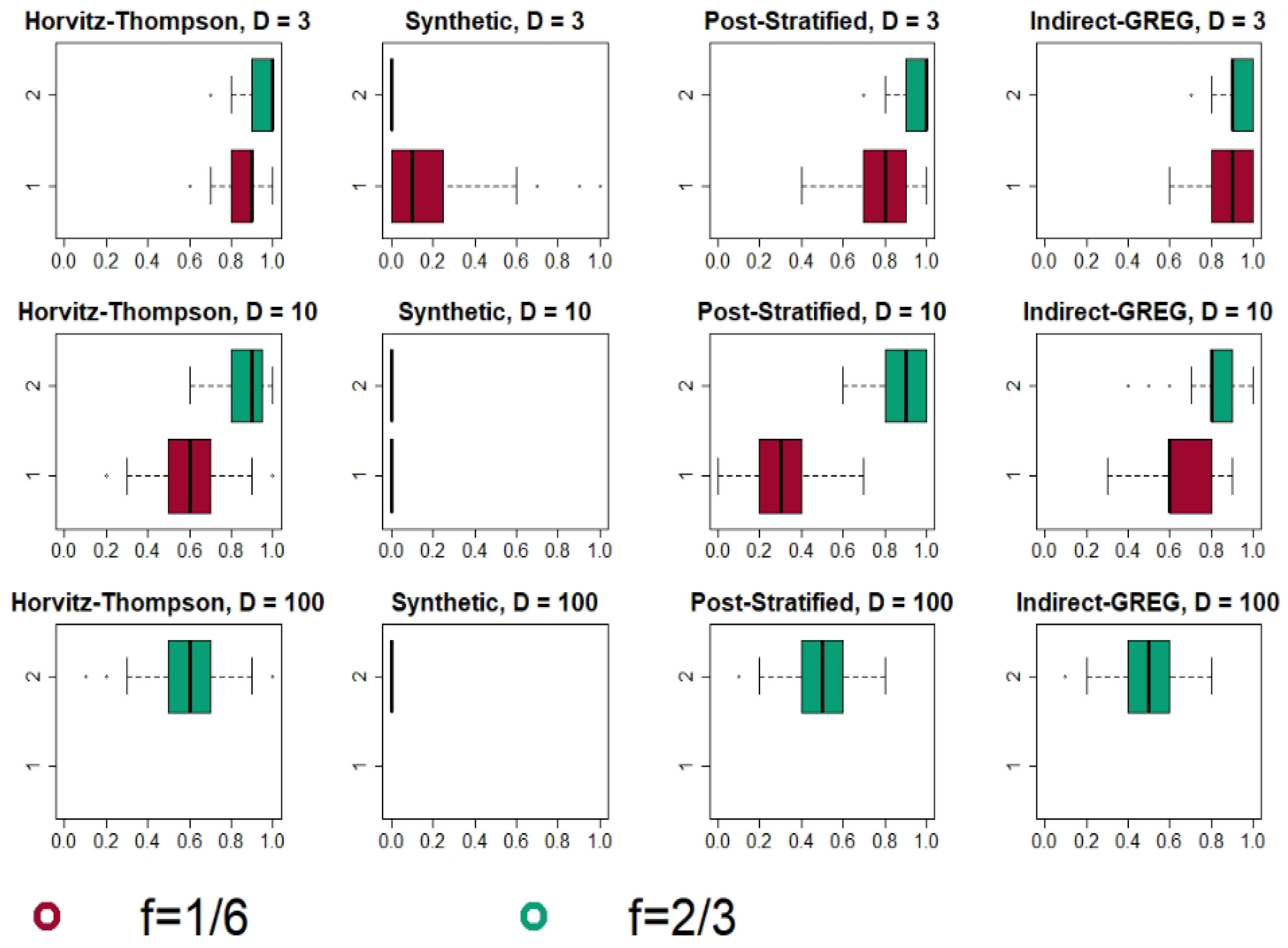
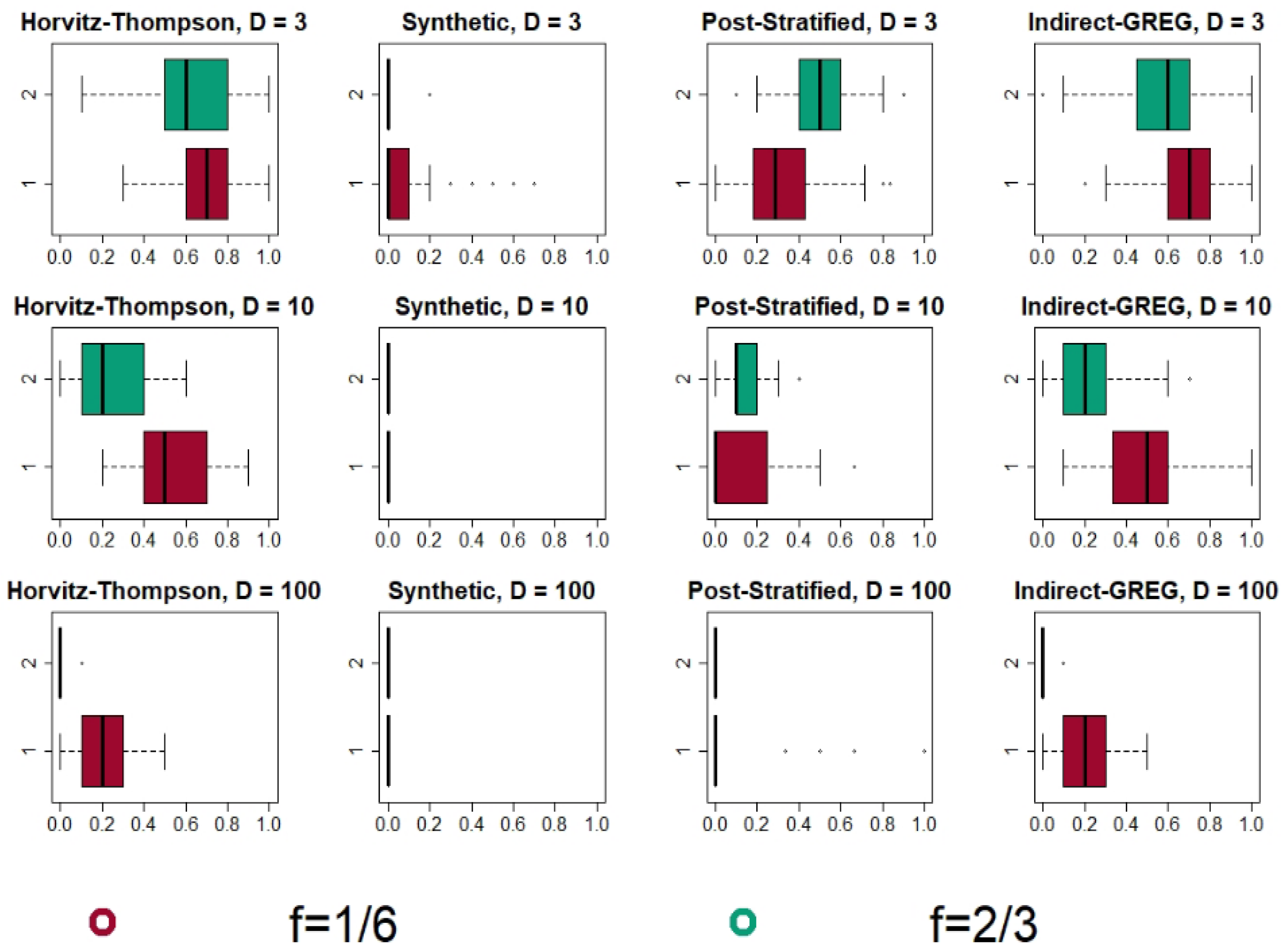
4.2.1. Bonferroni and Šidák Method: Results and Analysis

Recall that the Bonferroni correction introduced in [15] was originally proposed for a linear combination of normally distributed means; when variances were estimated, the t-distribution was suggested. Similarly, ref. [16] considered the means of multivariate normal distributions when the variances were known or at least equal; in the latter case, again the t-distribution was suggested for the critical values.

In the following figures, we compare boxplots for the Bonferroni-SCI coverages obtained for the different estimators and designs; see Figure 1 for the SRSWOR design and Figure 2 for the more complex UP design. For the Šidák method, see the simulation averages summarized in

Table 1. Coverage probabilities for all methods and estimators in various scenarios under SRSWOR. X∼$U7[0,10]$ for lines 8, 7, 11, 12; otherwise, X∼$U[0,1]$. Estimators are H-T: Horvitz–Thompson, D-G: direct-GREG, Syn: synthetic, P-S: post-stratified, I-G: indirect-GREG.

f	Bonferroni					Šidák					Max-Type
	H-T	D-G	Syn	P-S	I-G	H-T	D-G	Syn	P-S	I-G	H-T	D-G	Syn	P-S	I-G
	${\sigma }_u$ = 2		D = 3
1/6	0.874	0.355	0.187	0.773	0.887	0.874	0.355	0.205	0.773	0.887	0.946	0.946	0.991	0.895	0.999
2/3	0.953	0.87	0	0.953	0.918	0.953	0.87	0	0.953	0.917	0.987	0.998	0.951	0.983	0.998
1/6	0.865	0.355	0.546	0.677	0.869	0.864	0.355	0.565	0.676	0.869	0.948	0.969	0.986	0.914	1
2/3	0.946	0.87	0.015	0.926	0.943	0.945	0.87	0.014	0.926	0.942	0.992	1	0.687	0.987	1
	${\sigma }_u$ = 0.02
1/6	0.873	0.355	0.971	0.773	0.902	0.873	0.355	0.978	0.773	0.902	0.952	0.954	0.995	0.895	1
2/3	0.948	0.87	0.572	0.953	0.932	0.948	0.87	0.57	0.953	0.929	0.978	1	0.956	0.983	1
1/6	0.869	0.355	0.912	0.677	0.872	0.867	0.355	0.919	0.676	0.871	0.943	0.971	0.993	0.914	1
2/3	0.946	0.87	0.015	0.926	0.943	0.945	0.87	0.014	0.926	0.942	0.992	1	0.687	0.987	1
	${\sigma }_u$ = 2		D = 10
1/6	0.63	0.017	0	0.274	0.654	0.629	0.017	0	0.274	0.654	0.949	0.87	1	0.947	0.993
2/3	0.88	0.73	0	0.873	0.825	0.88	0.729	0	0.872	0.824	0.991	1	0.731	0.992	0.999
	${\sigma }_u$ = 0.02
1/6	0.618	0.017	0.708	0.274	0.701	0.616	0.017	0.724	0.274	0.7	0.951	0.879	1	0.947	0.999
2/3	0.868	0.73	0.005	0.873	0.855	0.867	0.729	0.005	0.872	0.855	0.99	1	0.61	0.992	1
	${\sigma }_u$ = 2		D = 50
1/6	0.142	0	0	0	0.171	0.141	0	0	0	0.171	0.977	1	1	0.964	0.998
2/3	0.724	0.448	0	0.661	0.637	0.724	0.446	0	0.66	0.636	0.984	1	0.007	0.999	1
	${\sigma }_u$ = 0.02
1/6	0.105	0	0	0	0.224	0.105	0	0	0	0.223	0.962	1	1	0.964	1
2/3	0.703	0.448	0	0.661	0.647	0.701	0.446	0	0.66	0.645	0.987	1	0.006	0.999	1
	${\sigma }_u$ = 2		D = 100
1/6	0.019	0	0	0	0.039	0.019	0	0	0	0.039	0.973	1	1	0.962	0.988
2/3	0.582	0.257	0	0.511	0.508	0.578	0.253	0	0.51	0.506	0.988	1	0	0.993	1
	${\sigma }_u$ = 0.02
1/6	0.008	0	0	0	0.052	0.008	0	0	0	0.051	0.96	1	1	0.962	0.998
2/3	0.577	0.257	0	0.511	0.549	0.575	0.253	0	0.51	0.547	0.995	1	0	0.993	1

. The boxplots roughly indicate the distributions of the joint coverages of all domain parameters over the $K=100$ populations. From these illustrations of medians and spreads of achieved coverages, we discover serious undercoverage which converges to zero quite rapidly for increasing D. Simulations for X∼$U[0,10]$ reveal no additional findings, so it is sufficient to look at variations of ${\sigma }_u$, f, D, n and N.

It becomes immediately clear that in using Bonferroni or Šidák, we achieve the wanted joint coverage of $95\%=1-\alpha$ only for the H-T estimator in the simple SRSWOR design, but even there only when considering just three domains with high sampling rates. When looking at the other estimators, we obtain worse results. For direct-GREG and our synthetic estimators, Bonferroni fails to provide appropriate coverage probabilities in almost all cases. So, either the variance estimates or the t-approximations do not work sufficiently well. For the synthetic estimator, it is also likely that the total estimator itself does not work well unless $n_d$ is sufficiently large in all domains. At first glance, P-S and I-GREG estimators perform somewhat better. But this holds only for the least interesting case with $D=3$. From the table, we see that there is not much difference in the coverage between SCIs constructed by Bonferroni versus Šidák.

For the UP design, we see that things become much worse. It is a bit surprising that the coverage is sometimes better for the low sampling rate than for the high one. But no estimator delivers an appropriate joint coverage, and the results are again “best” for the H-T. Our findings do not vary over the considered simulation designs although the numerical outcomes do, especially when increasing the ratio f. Not shown is that simulation outcomes became much worse when the random effects u and $ϵ$ deviated from normality.

In sum, Bonferroni and Šidák SCI (which are typically considered as conservative methods, i.e., they should lead to overcoverage) fail almost always. Then, comparative or joint inference for domains is impossible for any set of $D>3$ domains based on these methods even in the most simple setup and estimation problem. For understanding the failures, it is worth recalling that increasing the number of domains has two effects: the risk that some domains have a very small $n_d$ increases, and at the same time we have to cover an increasing number of ${\theta }_d$. It is increasingly likely that one interval does not contain its ${\theta }_d$, unless all ${\widehat{\theta }}_d$ exhibit good variance estimates and obey the t-distribution. The quality of the variance estimates has been studied extensively in the literature. Let us therefore have a closer look at the problem of taking as critical values the quantiles of the t-distribution. Clearly, the quality of distributional approximation depends on the $n_d$, $d=1,\dots ,D$, but also on the estimators and the distribution of $y_k$; if its shape is very skewed (and/or has heavy tails), an approximation by t requires a much larger $n_d$ in all domains than would be the case for symmetric ones [20] (with slim tails). From Figure 3, we see that in this sense, our simulation setting is quite favourable for the Bonferroni and Šidák corrections. One may ask why we nonetheless obtain those bad results. Figure 4 gives an answer for the H-T estimates on which we built the SCIs. While the majority of domain estimates fit well to the normal distribution, in several domains the true distribution is far from it; those destroy the joint coverage. This is even more emphasised for other estimators (figures not shown).

Consequently, Bonferroni and Šidák corrections with t-quantiles cannot work. An alternative for obtaining the quantiles needed for the critical values could be to estimate the distribution by bootstrap. Unfortunately, while this may work for quantiles $q_{1-\alpha /2}$ with $\alpha =0.1$, $0.5$ or $0.01$, for Bonferroni, we need quantiles with ${\alpha }^{\prime }=\alpha /D$, which become extremely small as D increases. The bootstrap estimates of those quantiles are not reliable unless the $n_d$ or f become very large. For $D>10$, one may easily obtain situations in which one needs more bootstrap samples than different samples exist, leaving computational issues apart. Thus, while bootstrap for estimating critical values is interesting, it is not helpful in combination with the Bonferroni or Šidák corrections.

Clearly, for increasing sample sizes or sampling rate f, the problem might be less emphasised, depending on the underlying distribution of Y and the wanted estimator. In practice, this could become quite costly, but we conducted a simulation which considered larger N and larger n for the same data generating process as described above; see

Table 2. Coverage probabilities for 95% SCI when using the Horvitz–Thompson estimator with the Bonferroni correction under SRSWOR.

	D = 5	D = 10	D = 50
N	1000	2000	10,000
n	750	1500	8500
f	0.75	0.75	0.85
Coverage	0.93	0.92	0.9

. While one may argue that the coverage probabilities in this example are not too bad, we still observe divergence, not convergence. Moreover, recall that we simulated a quite favourable situation with $y_k$ and estimators not being too far from normality. In the Supplementary Materials, we briefly discuss what the literature tells us about the sample sizes needed for a reasonable approximation of a simple mean estimate by normality when Y is not normal. It can be seen there how dramatically $n_d$ must increase in all domains to achieve this when the distribution of Y becomes more skewed. We conclude that one needs a sampling design that accounts for the partitioning of the population into domains and guarantees large sample sizes and/or a high sampling rate in each domain. By controlling the sampling rate within each domain, we are no longer in a standard situation in practice. Moreover, if some of the $N_d$ are small, then this solution also would fail.

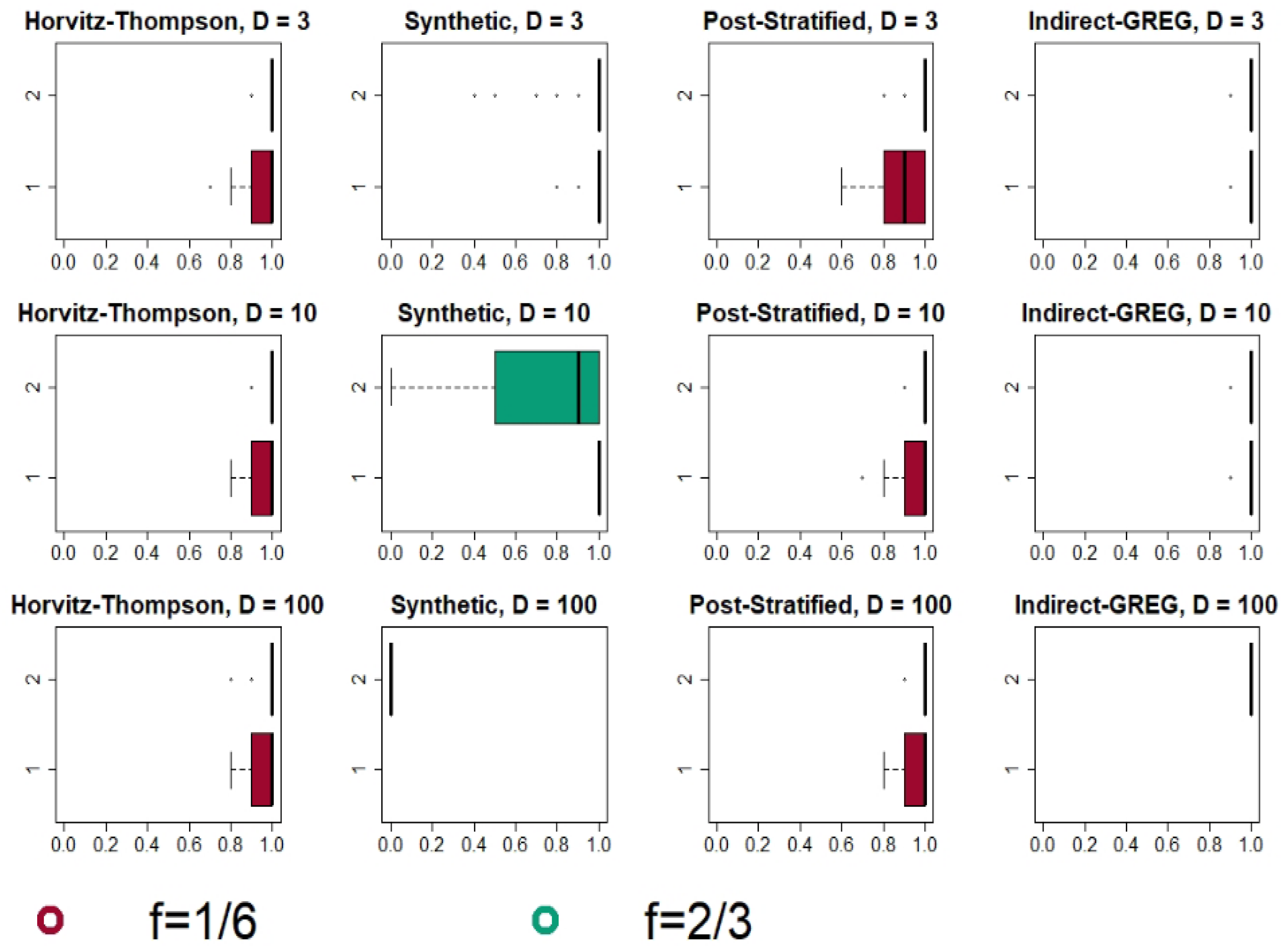
4.2.2. Max-Type Statistic with Bootstrap and an Overall Comparison

We now pursue the idea of using bootstrap for approximating the critical values, combining it with the approach of performing uniform inference via max-type statistics; recall Section 2. Results under SRSWOR are summarized in Table 1. We see that we are much closer to the nominal level of $1-\alpha$ than before. For the sake of comparison, we repeat the exercise of the last subsection, showing in Figure 5 the distributions of coverage probabilities for the max-type SCIs. Comparing this with Figure 1, we observe that the distributions are more concentrated on the right. We also observe that in most cases, the spread of the boxes is much smaller. Finally, we observe that in some situations the max-type approach leads to overcoverage, which was never the case before.

Again, the SCIs for the direct-GREG and the synthetic estimator almost never have the desired coverage. Like for the Bonferroni method, this may be due to the large variation in these estimators. For the H-T and the P-S estimators, we obtain reasonable results, except for the latter when $D=3$. However, in several situations, the coverage is larger than $1-\alpha$, in particular for the I-GREG, which is therefore not recommendable. We conclude that for $D\le 10$ one would recommend constructing SCIs by max-type statistics of H-T estimators and for $D>10$ alternatively by the P-S estimators.

As the estimates and their corresponding variances are the same for all methods, the main difference to the above in our new SCI construction is the way we calculate the critical values. In

Table 3. Critical values of 95% SCI for the Bonferroni and the max-type approaches using the Horvitz–Thompson estimator under SRSWOR.

	D = 3					D = 10					D = 50
f	0.25	0.5	0.75	0.8	0.9	0.25	0.5	0.75	0.8	0.9	0.25	0.5	0.75	0.8	0.9
Max-Type	2.56	2.63	2.88	3.03	3.65	3.35	3.2	3.43	3.36	3.75	4.32	3.86	4.16	4.91	4.57
Bonferroni	2.42	2.41	2.4	2.4	2.4	2.82	2.81	2.81	2.81	2.81	3.29	3.29	3.29	3.29	3.29

, we compare these when using the max-type statistic and the Bonferroni correction, respectively, both for the H-T estimator. As expected, for $D=3$, they differ only a bit, substantially depending on the sampling rate f. For increasing D, the difference between them becomes more and more substantial.

Results for the UP design are displayed in

Table 4. Coverage probabilities for all methods and estimators in various scenarios for an unequal probability design UP and X∼$U[0,1]$. Estimators are H-T: Horvitz–Thompson, Syn: synthetic, P-S: post-stratified, I-G: indirect-GREG.

f	Bonferroni				Šidák				Max-Type
	H-T	Syn	P-S	I-G	H-T	Syn	P-S	I-G	H-T	Syn	P-S	I-G
	${\sigma }_u$ = 2		D = 3
1/6	0.713	0.08	0.3183	0.7065	0.713	0.08	0.3183	0.70355	0.883	0.297	0.8404	0.99
2/3	0.625	0.002	0.492	0.569	0.624	0.002	0.489	0.568	0.843	0.067	0.804	0.923
	${\sigma }_u$ = 0.02
1/6	0.727	0.773	0.291	0.671	0.726	0.773	0.291	0.667	0.894	0.793	0.836	1
2/3	0.628	0.428	0.492	0.497	0.625	0.426	0.489	0.497	0.851	0.538	0.804	0.962
	${\sigma }_u$ = 2		D = 10
1/6	0.532	0	Na	0.469	0.531	0	Na	0.464	0.884	0.009	Na	1
2/3	0.253	0	0.151	0.229	0.25	0	0.151	0.229	0.905	0.002	0.863	0.961
	${\sigma }_u$ = 0.02
1/6	0.507	0.51	0.078	0.476	0.505	0.508	0.0779	0.473	0.889	0.526	0.739	1
2/3	0.269	0.058	0.151	0.126	0.268	0.058	0.151	0.123	0.905	0.179	0.863	0.987
	${\sigma }_u$ = 2		D = 50
1/6	0.287	0	Na	0.316	0.286	0,00	Na	0.315	0.8	0.003	Na	1
2/3	0.004	0.001	0	0.004	0.004	0	0	0.004	0.946	0.001	0.926	0.946
	${\sigma }_u$ = 0.02
1/6	0.367	0.021	Na	0.367	0.367	0.02	Na	0.367	0.794	0.2882	Na	0.794
2/3	0.005	0.001	0	0	0.005	0.001	0	0	0.934	0.019	0.926	0.995
	${\sigma }_u$ = 2		D = 100
1/6	0.197	0	Na	0.289	0.197	0,00	Na	0.286	0.651	0.009	Na	1
2/3	0.001	0	0	0	0.001	0	0	0	0.964	0	0.93	0.991
	${\sigma }_u$ = 0.02
1/6	0.286	0.004	Na	0.361	0.282	0.0043	Na	0.358	0.65	0.4243	Na	1
2/3	0	0.001	0	0	0	0.001	0	0	0.957	0.007	0.93	0.994

. Again, the real coverage is much closer to the desired level for the “max-type with bootstrap” method than for the classical approaches. However, we obtain the desired coverage for almost all simulations only for the I-GREG estimator. As for the SRSWOR design, the max-type SCIs are too conservative when the number of domains increases but the sampling rate decreases. For the H-T estimator, we observe that, as the number of domains increases and the sampling rate is high, the coverage becomes better. For $D=50$ and $D=100$, we obtain the desired coverage probability. We also observe a similar pattern for the P-S estimator. Finally, the SCI for Syn fails in all situations. These findings are coherent with the ones previously found for a SRSWOR design. The “Na” indicate that in some crossed group-domains $U_{dg}$ we do not have data.

Even though we briefly commented above on it, let us add some comments on the seemingly quite-frequent overcoverage of the max-type statistic-based SCIs. There are two major comments on this issue and some smaller ones. First, the max-type-based approach tries to construct SCIs that account for the worst case. Intuitively, this suggests that these SCIs tend to have overcoverage; one may even argue that this would be suboptimal. However, our aim was not to invent new methods at this stage. We rather wanted to study how well-known methods work when employed to construct SCIs for frequently used direct and indirect domain estimators. Second, the max-type approach is particularly sensitive to the quality of variance estimators; recall statistic Equation (3). To what we found, these work particularly badly for the direct-GREG and indirect-GREG approaches but are also problematic for the synthetic one. Certainly, the choice of the bootstrap method also can play a role, but here we cannot generally blame the bootstrap for over- or undercoverage.

How large the SCIs are in practice and how well they separate domain parameters significantly depends on many factors, like sample size, sample rate, the distribution of the estimator and in particular its variance. How reasonable they are, and consequently conducting comparative statistics between domains at all, depends also on the ratio of the within-domain variation compared to the between-domain variation. In brief, there is no generally valid answer to this. If in practice it is noted that constructing SCIs for a large number D of domains gives extremely large and therefore useless intervals, then one should concentrate on small but interesting subsets of domains and construct the SCIs for them (reducing D). The simulation design may look a bit artificial but was constructed this way to see the different effects not only of sample size and the complexity of sample design but also of size, within versus between variation, etc.

In the following, we present a small simulated (now visual) illustration before we turn to the real data example. We concentrate on max-type-based SCIs for the H-T estimators of domain totals with our different sampling rates and sampling designs. Let us first consider $D=10$ domains simultaneously. For a better illustration, the variable of interest is now generated by

$$y_{kd}=0.2+4x_{kd}+u_d+e_{kd},k=1,\dots ,N_d,d=1,\dots ,10,$$

where $x_{kd}$ are, as before, uniformly distributed on $[0,10]$, $u_d=10d$ are the domain intercepts (not randomly drawn) to control the between-domain variation and $e_{kd}$ are normally distributed noise with mean 0 and standard deviation equal to $x_{kd}$. The latter was performed for obtaining a reasonable UP design whose weights are determined out of the dependence between y and x; a too-low relation results in worse estimators and larger SCIs for the UP design. The domain population size is set to $N_d=120$ for all domains. The sampling rates are set such that the sample sizes are $n\in \{200,500\}$.

Figure 6 plots the SCIs obtained from one simulation run. We see that the SCIs are reasonably small and therefore useful throughout when the total sample size is $n=500$. For the much smaller sample size, we observe quite large SCIs, at least for the domains with large values for their $y_{kd}$. The results are less promising for the UP design which, however, is also due to the small relation between y and x.

Next, we consider an example for $D=50$ domains with sample sizes $n\in \{1000,2500\}$. The data are generated from the same process as above but now with domain intercepts $u_d=u_{d-1}+2$, where $u_1=1$. The resulting SCIs of one simulation run are plotted in Figure 7. Here, we observe a similar situation as before, but even less favourable for the small sample situation, and just uninformative SCIs for the UP design. However, even for $D=50$, the SCIs are reasonably short for many domains when the total sample size is 2500.

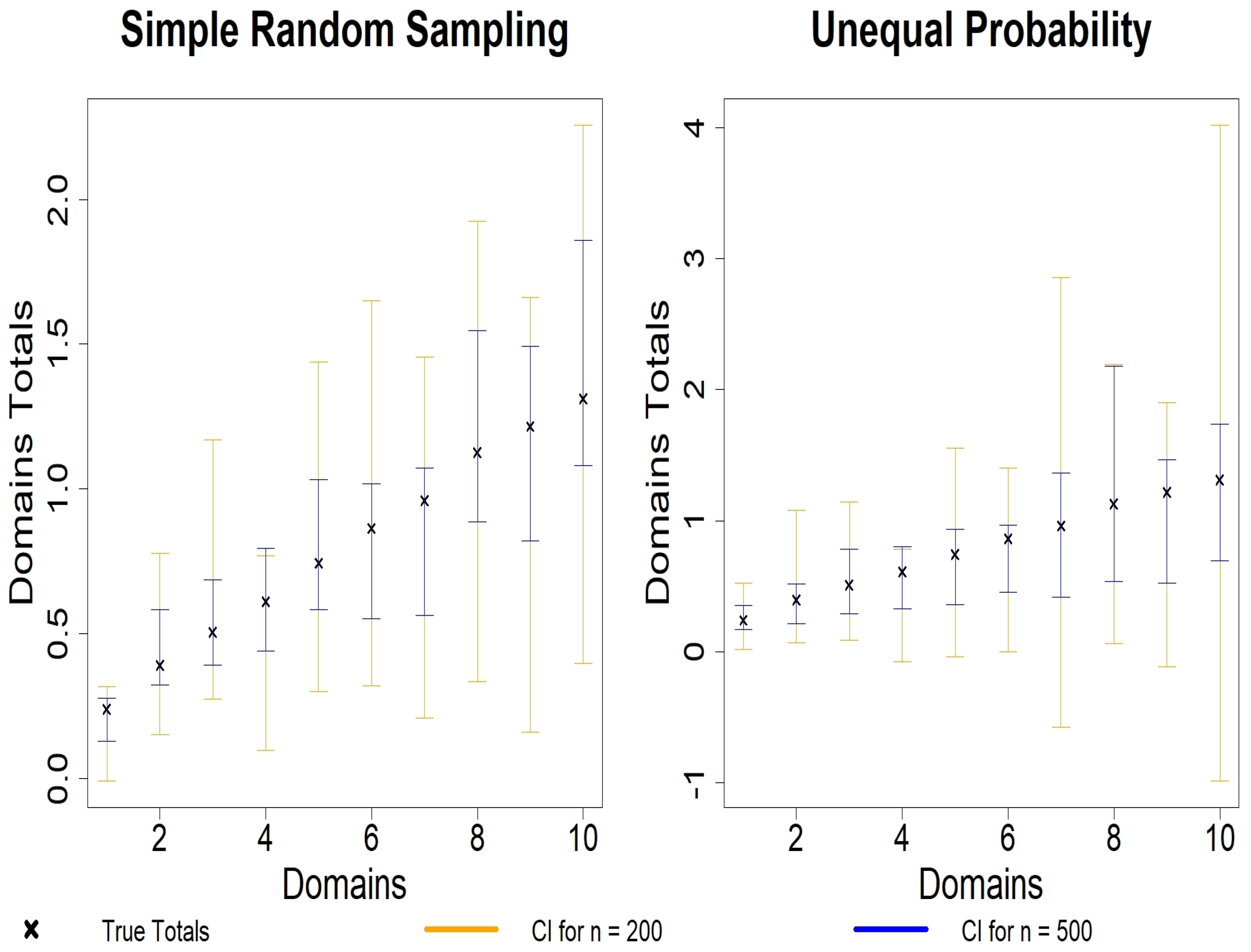
5. Estimating Total Tax Incomes: A Simulation Study with Belgian Data

In this section, we conduct a simulation study that is based on real data. We consider the Belgian Municipalities Population set provided in the R package sampling [24]. It contains data on incomes in the Belgian municipalities for 2003 and 2004. Our $y_d$ of interest is the total taxable income in each of the $N=589$ municipalities.

The provided auxiliary information here is the total population Tot04 in each municipality, $x_1$, and the total number of women Women04 in each municipality, $x_2$, both for 2004. The kernel density of taxable income is shown in Figure 8; it exhibits a strongly skewed distribution that even after taking the logarithm does not become symmetric. The population U of municipalities is partitioned in $D_1=9$ domains that correspond to the Belgian provinces and in $D_2=93$ that correspond to the arrondissements. Our methods will be studied in both cases: when the 9 domains are of interest and afterwards for the situation when the 93 domains are of interest. We consider sample size $n^1=85$, which corresponds to $f_1\approx 1/6$, and $n^2=335$, which gives $f_2\approx 2/3$.

Again, we use a SRSWOR sampling design: all the first- and second-order inclusion probabilities are known to be ${\pi }_k=n^i/N,{\pi }_{k\ell }=n^i(n^i-1)/N(N-1),i=1,2$. Based on the findings of the above sections, we concentrate on the H-T and the I-GREG estimators, respectively. The former is still the most considered one in survey methodology, performs best in our simulations and is also applied to compute the GREG; recall Equation (11). The latter was chosen due to its performance in Section 4. Results are summarized in

Table 5. Uniform coverage probabilities for the Belgian Municipalities Population dataset.

	Provinces						Arrondissements
	Bonferroni		Šidák		Max-Type		Bonferroni		Šidák		Max-Type
	H-T	I-GREG	H-T	I-GREG	H-T	I-GREG	H-T	I-GREG	H-T	I-GREG	H-T	I-GREG
$n^1$	0.3647	0.4138	0.3637	0.4124	0.9618	1	0.0917	0.0196	0.091	0.0196	0.9019	0.9679
$n^2$	0.4824	0.606	0.4813	0.6054	0.9753	1	0.0206	0.0292	0.0204	0.0291	0.9677	0.9998

and Figure 9, the latter indicating the sample distribution of the estimators for $D_1=9$.

Our results confirm the ones found in Section 4. The Bonferroni and Šidák corrections do not work as they never succeed in jointly covering the set of estimates and the coverage is lower when the sample size decreases or the number of domains increases. In contrast, our max-type approach is able to deliver a joint coverage that is at least close to the nominal level, except for the situation of a large number of domains with small sample sizes when using the H-T estimator for constructing SCIs. In conclusion, for the SCIs of the totals and mean or linear functions of them, we recommend using the max-type method with a bootstrap algorithm suitable for finite populations and a specific sampling design, in combination with H-T and I-GREG.

6. Discussion and Conclusions

Even though the literature on methods for domain and small area estimation has evolved amazingly over the last decades, little attention has been given to the problem of comparative or simultaneous analysis for them. But today, domain estimates are increasingly often used for resource allocation, i.e., redistribution or joint allocations under budget constraints. This requires simultaneous comparisons for at least some subsets of domains. For valid inference, we should then offer multiple tests or confidence intervals. Just recently, this was performed in the context of mixed model-based small area estimation [11,12,14]. To the best of our knowledge, we are the first who consider this problem for direct and indirect domain estimators which are still in frequent use. A reason for this gap in the literature could be that people may have relied on standard devices like the well-known Bonferroni correction. Our article shows, however, that simple standard devices fail, not only for large D, but already for $D>3$. Moreover, for an increasing number of domains, the size $n_d$ of all domain samples must grow significantly if one wants to guarantee the functioning of those standard devices. In practice, the Bonferroni and Šidák corrections can therefore not be recommended. In contrast, for linear indicators, we succeed in showing that the max-type statistics approach works very well if equipped with an appropriate bootstrap. One could further think about alternative refined Bonferroni methods. However, we have seen that the original, typically too-conservative method does not lead to over- but to undercoverage. Consequently, one would directly resort to bootstrap confidence intervals. Combining this idea with the max-type statistic for uniform inference provides us with reasonably well-working SCIs. An R package for constructing those SCIs is in preparation.

References

1. Pfeffermann, D. New Important Developments in Small Area Estimation. Stat. Sci. 2013, 28, 40–68. [Google Scholar] [CrossRef]
2. Tillé, Y. Sampling and Estimation from Finite Populations; Wiley Series in Survey Methodology; John Wiley & Sons: Hoboken, NJ, USA, 2020. [Google Scholar]
3. Morales, D.; Lefler, M.D.E.; Pérez, A.; Hobza, T. A Course on Small Area Estimation and Mixed Models; Statistics for Social and Behavioral Sciences; Springer: Berlin/Heidelberg, Germany, 2021. [Google Scholar]
4. Little, R. To model or not to model? Competing modes of inference for finite population sampling. J. Am. Stat. Assoc. 2004, 99, 546–556. [Google Scholar] [CrossRef]
5. Stanke, H.; Finley, A.; Domke, G. Simplifying Small Area Estimation With rFIA: A Demonstration of Tools and Techniques. Front. For. Glob. Chang. 2022, 5. [Google Scholar] [CrossRef]
6. Lohr, S. Sampling: Design and Analysis; Chapman and Hall, CRC Press: New York, NY, USA, 2019. [Google Scholar] [CrossRef]
7. Eurostat. Guidelines on Small Area Estimation for City Statistics and Other Functional Geographies; European Union: Maastricht, The Netherlands, 2019. [Google Scholar]
8. Tzavidis, N.; Zhang, L.C.; Luna, A.; Schmid, T.; Rojas-Perilla, N. From start to finish: A framework for the production of small area official statistics. J. R. Statist. Soc. A 2018, 181, 927–979. [Google Scholar] [CrossRef]
9. Hochberg, Y.; Tamhane, A. Multiple Comparison Procedures; John Wiley & Sons: New York, NY, USA, 1987. [Google Scholar]
10. Romano, J.; Wolf, M. Exact and approximate stepdown methods for multiple hypothesis testing. J. Am. Stat. Assoc. 2005, 100, 94–108. [Google Scholar] [CrossRef]
11. Reluga, K.; Lombardía, K.; Sperlich, S. Simultaneous Inference for Empirical Best Predictors with a Poverty Study in Small Areas. J. Am. Stat. Assoc. 2023, 118, 583–595. [Google Scholar] [CrossRef]
12. Reluga, K.; Lombardía, K.; Sperlich, S. Simultaneous Inference for linear mixed model parameters with an application to small area estimation. Int. Stat. Rev. 2023, 91, 193–217. [Google Scholar] [CrossRef]
13. Burris, K.; Hoff, P. Exact Adaptive Confidence Intervals for Small Areas. J. Surv. Stat. Methodol. 2020, 8, 206–230. [Google Scholar] [CrossRef]
14. Kramlinger, P.; Krivobokova, T.; Sperlich, S. Marginal and Conditional Multiple Inference for Linear Mixed Model Predictors. J. Am. Stat. Assoc. 2023, 118, 2344–2355. [Google Scholar] [CrossRef]
15. Dunn, O.J. Multiple Comparisons Among Means. J. Am. Stat. Assoc. 1961, 56, 52–64. [Google Scholar] [CrossRef]
16. Šidák, Z. Rectangular confidence regions for the means of multivariate normal distributions. J. Am. Stat. Assoc. 1967, 62, 626–633. [Google Scholar]
17. Chauvet, G. Méthodes de Bootstrap en Population Finie. Ph.D. Thesis, Université de Rennes 2, Incheon, Republic of Korea, 2007. [Google Scholar]
18. Estevao, V.M.; Särndal, C.E. Borrowing Strength Is Not the Best Technique Within a Wide Class of Design-Consistent Domain Estimators. J. Off. Stat. 2004, 20, 645–669. [Google Scholar]
19. Horvitz, D.G.; Thompson, D.J. A generalization of sampling without remplacement from a finite universe. J. Am. Stat. Assoc. 1952, 47, 663–685. [Google Scholar] [CrossRef]
20. Särndal, C.E.; Swensson, B.; Wretman, J. Model Assisted Survey Sampling, 1st ed.; Springer Series in Statistics; Springer Inc.: New York, NY, USA, 1992. [Google Scholar]
21. Ghosh, M.; Rao, J. Small Area Estimation: An Appraisal. Stat. Sci. 1994, 9, 55–93. [Google Scholar] [CrossRef]
22. Hájek, J. Discussion of an essay on the logical foundations of survey sampling, part ones by D. Basu. In Foundations of Statistical Inference; Godambe, V.P., Sprott, D.A., Eds.; Toronto, Holt, Rinehart and Winston of Canada: Toronto, ON, Canada, 1971. [Google Scholar]
23. Lehtonen, R.; Veijanen, A. Design-Based Methods of Estimation for Domains and Small Areas; Handbook of Statistics; Elsevier B.V.: Amsterdam, The Netherlands, 2009; Volume 29B, Chapter 31; pp. 219–249. [Google Scholar]
24. Tillé, Y.; Matei, A. Sampling: Survey Sampling; R Package Version 2.9. 2021. Available online: https://cran.r-project.org/web/packages/sampling/index.html (accessed on 8 February 2024).
Figure 1. Boxplots of uniform coverage probabilities for all estimators when σ u = 2 , X U [ 0 , 1 ] under SRSWOR and applying the Bonferroni correction for 95% SCI.
Stats 07 00020 g001
Figure 2. Boxplots of uniform coverage probabilities for all estimators when σ u = 2 , X U [ 0 , 1 ] under UP design and applying the Bonferroni correction for 95% SCI.
Stats 07 00020 g002
Figure 3. Densities of Y for different sampling rates with σ u = 2 , X U [ 0 , 1 ] under SRSWOR. The normal distribution with the same parameters is plotted in grey.
Stats 07 00020 g003
Figure 4. Densities of the Horvitz–Thompson estimates for different simulation designs under SRSWOR. Each domain estimate is plotted in a different colour.
Stats 07 00020 g004
Figure 5. Boxplots of the uniform coverage probabilities for all estimators under different simulation designs with σ u = 2 under SRSWOR, when applying the max-type statistics approach combined with bootstraps for finite populations for constructing 95% SCI.
Stats 07 00020 g005
Figure 6. Plots of max-type-based SCIs for D = 10 with Horvitz–Thompson estimator.
Stats 07 00020 g006
Figure 7. Plots of max-type-based SCIs for D = 50 with Horvitz–Thompson estimator.
Stats 07 00020 g007
Figure 8. Density of total taxable income.
Stats 07 00020 g008
Figure 9. Densities of the Horvitz–Thompson estimator in each of the 9 provinces. Some are close to a normal distribution, but others display asymmetric or bimodal distributions.
Stats 07 00020 g009