Abstract
Tensor product smoothers are frequently used to include interaction effects in multiple nonparametric regression models. Current implementations of tensor product smoothers either require using approximate penalties, such as those typically used in generalized additive models, or costly parameterizations, such as those used in smoothing spline analysis of variance models. In this paper, I propose a computationally efficient and theoretically precise approach for tensor product smoothing. Specifically, I propose a spectral representation of a univariate smoothing spline basis, and I develop an efficient approach for building tensor product smooths from marginal spectral spline representations. The developed theory suggests that current tensor product smoothing methods could be improved by incorporating the proposed tensor product spectral smoothers. Simulation results demonstrate that the proposed approach can outperform popular tensor product smoothing implementations, which supports the theoretical results developed in the paper.
1. Introduction
Consider a multiple nonparametric regression model [1] of the form
where is the observed response variable, is the observed predictor vector, is the product domain with denoting the domain of the j-th predictor, is the (unknown) real-valued function connecting the response and predictors, and is an error term that satisfies and . Note that this implies that , i.e., the function is the conditional expectation of the response variable Y given the predictor vector . Given a sample of training data, the goal is to estimate the unknown mean function f without having any a priori information about the parametric nature of the functional relationship (e.g., without assuming linearity).
Let denote a sample of n independent observations from the model in Equation (1), where is the i-th observation’s realization of the response variable, and is the i-th observation’s realization of the predictor vector. To estimate f, it is typical to minimize a penalized least squares functional of the form
where denotes some non-negative penalty that describes the complexity of f, i.e., if , then the function f is more complex (less smooth) than the function g, and the tuning parameter controls the influence of the penalty. To find a reasonable balance between fitting (the data) and smoothing (the function), is often chosen via cross-validation, information theory, or maximum likelihood estimation [2].
When the penalty P is a semi-norm in a (tensor product) reproducing kernel Hilbert space (RKHS), the minimizer of Equation (2) is referred to as a (tensor product) smoothing spline [1,3,4,5,6,7]. Note that (tensor product) smoothing splines are used within multiple nonparametric regression frameworks, such as generalized additive models (GAMs) [7,8] and smoothing spline analysis of variance (SSANOVA) models [3,5,6]. Such methods have proven powerful for nonparametric (multivariate) function estimation for a variety of different types of data, such as oceanography [9], social media [10], clinical biomechanics [11], self-esteem development [12], smile perception [13], clinical neuroimaging [14], psychiatry [15], and demography [16].
To find the that minimizes Equation (2), it is first necessary to specify the assumed model form. For example, with predictors, we could consider one of two forms:
where is the bidimensional predictor, is an intercept, is the main effect of the first predictor, is the main effect of the second predictor, and is the two-way interaction effect. Note that these models are nested given that the additive model is equivalent to the interaction model if .
For additive models, is typically represented by a spline basis of rank , such as . Note that denotes the known spline basis vector that depends on the chosen knots (later described), and is the unknown coefficient vector. To define the complexity of each (additive) effect, it is typical to consider penalties of the form , where is a semi-positive definite matrix. Using these representations of the function evaluation and penalty, Equation (2) can be written as
where is the i-th observation’s realization of the vector, and are tuning parameters that control the influence of each penalty.
When the model contains interaction effects, different approaches can be used to represent and penalize the interaction terms. In GAMs, it is typical to (i) represent interaction effects by taking an outer (Kronecker) product of marginal basis vectors, and (ii) penalize interaction effects using an equidistant (grid) approximation (see [7] (pp. 227–237)). In SSANOVA models, it is typical to represent and penalize interaction effects using a tensor product RK function (see [5] (pp. 40–48)). For a thorough comparison of the two approaches, see Helwig [1]. In both frameworks, estimation of interaction effects can be costly when using a moderate to large number of knots, which is true even when using scalable parameterizations and algorithms [9,17,18]. This is because efficient computational tools for exact tensor product function representation and penalization are lacking from the literature, which hinders the widespread application of tensor product smoothing splines.
To address this practical issue, this paper (i) proposes a spectral representer theorem for univariate smoothing spline estimators, and (ii) develops efficient computational strategies for constructing tensor product smoothing splines from marginal spectral representations. The marginal spectral spline representation that I propose is similar to that proposed by [19]; however, the version that I consider penalizes all of the non-constant functions of each predictor. The tensor product basis construction approach that I propose generally follows the idea proposed by [20], where tensor products are built from outer (Kronecker) products of marginal bases. However, unlike this approach, I leverage reproducing kernel theory to develop exact analytical penalties for tensor product smooth terms. The proposed approach makes it possible to fit tensor product smoothing spline models (a) with interaction effects between any combination of predictors, and (b) using any linear mixed modeling software.
The remainder of this paper is organized as follows: Section 2 provides background on the reproducing kernel Hilbert space theory relevant to univariate smoothing splines; Section 3 provides background on the tensor product smoothing splines; Section 4 proposes an alternative tensor product smoothing spline (like) framework that penalizes all non-constant functions of the predictor; Section 5 develops the spectral representer theories necessary for efficiently computing exact tensor product penalties; Section 6 conducts a simulation study to compare the proposed approach to an existing (comparable) method; Section 7 demonstrates the proposed approach using a real dataset; and Section 8 discusses potential extensions of the proposed approach.
2. Smoothing Spline Foundations
2.1. Reproducing Kernel Hilbert Spaces
Consider a single predictor (i.e., ) that satisfies , and let denote a RKHS of functions on . The unknown function f from Equation (2) is assumed to be an element of , which will be denoted by . Suppose that the space can be decomposed into two orthogonal subspaces, such as , where ⊕ denotes the tensor summation. Note that is the null space, which contains all functions (in ) that have zero penalty, and is the contrast space, which contains all functions (in ) that have a non-zero penalty. In some cases, the null space can be further decomposed, such as , where is a space of constant functions (intercept), and  is a space of non-constant functions (unpenalized). For example, when using a cubic smoothing spline, contains the linear effect of X, which is unpenalized.
is a space of non-constant functions (unpenalized). For example, when using a cubic smoothing spline, contains the linear effect of X, which is unpenalized.The inner product of will be denoted by for any , and the corresponding norm will be written as for any . Given the tensor sum decomposition of , the inner product can be written as a summation of the corresponding subspaces’ inner products, such as . Note that is the null space inner product for any , and is the contrast space inner product for any . The corresponding norms will be denoted by (norm of ) and (norm of ). When the null space consists of non-constant functions, i.e, when , the null space inner product can be written as , where is the inner product of for any , and is the inner product of for any . The corresponding norm can be written as , where and denote the norms of and , respectively.
The RK of will be denoted by for any . Note that the RK is an element of the RKHS, i.e., for any . By definition, the RK is the representer of the evaluation functional in , which implies that the RK satisfies for any and any . This important property, which is referred to as the “reproducing property” of the (reproducing) kernel function, implies that any function in can be evaluated through the inner product and RK function. Following the decompositions of the inner product, the RK function can be written as , where and denotes the RKs of and , respectively. Furthermore, when , the null space RK can be decomposed such as , where and denotes the RKs of and , respectively. By definition, for all , where is some constant.
The tensor sum decomposition implies that any function can be written as a summation of two components, such as
where is the null space contribution and is the contrast space contribution. Furthermore, when , the null space component can be further decomposed into its constant and non-constant contributions, such as , where for all . Let denote the projection operator for the null space, such that for any . Similarly, let denote the projection operator for the contrast space, such that for any . Note that is referred to as the “parametric component” of f, given that is a finite dimensional subspace. In contrast, is the “nonparametric component” of f, given that is an infinite dimensional subspace.
2.2. Representer Theorem
Still consider a single predictor (i.e., ) that satisfies with denoting a RKHS of functions on . Now, suppose that the penalty functional in Equation (2) is defined to be the squared norm of the function’s projection into the contrast space, i.e., . Note that the second equality is due to the fact that for any , which is a consequence of the orthogonality of and . More specifically, given , consider the problem of finding the function
where is the projection operator for the contrast space . Note that the solution is subscripted with to emphasize the dependence on the tuning parameter.
Suppose that the null space has dimension . Note that when only consists of the constant (intercept) subspace, whereas when . Let denote a basis for the null space , such that any can be written as for some coefficient vector . The representer theorem of Kimeldorf and Wahba [21] reveals that the optimal smoothing spline estimator from Equation (4) has the form
where is the RK of the contrast space, and is the coefficient vector that combines the training data RK evaluations.
The representer theorem in Equation (5) reveals that the smoothing spline estimator can be written as , where is the null space contribution and is the contrast space contribution. Using the optimal representation from Equation (5), the penalty has the form
where evaluates the RK function at all combinations of . Note that the first line is due to the fact that for any , the second line is due to the bilinear nature of the inner product, and the third line is due to the reproducing property of the RK function.
2.3. Scalable Computation
The optimal solution given by the representer theorem in Equation (5) uses all training data points to represent , which could be computationally costly when n is large. For more scalable computation, it is typical to approximate by evaluating the contrast space RK at all combinations of knots, which are typically placed at the quantiles of the training data predictor scores. Using this type of (low-rank) smoothing spline approximation, the approximation to the representer theorem becomes
where are the chosen knots. As long as enough knots are used in the representation, the approximate representer theorem in Equation (7) can produce theoretically optimal function estimates [22,23]. For optimal asymptotic properties, the number of knots should be on the order of , where depends on the smoothness of the unknown true function. Note that is necessary when is barely satisfied, whereas can be used when f is sufficiently smooth (see [5,22,23]).
Using the approximate representer theorem in Equation (7), the penalized least squares functional from Equation (4) becomes a penalized least squares problem of the form
where is the i-th observation’s null space basis function vector, and is the i-th observation’s contrast space basis function vector. Note that evaluates the contrast space RK at all combinations of knots. Given a choice of the smoothing parameter , the solution has the form
where is the null space design matrix with as rows, is the contrast space design matrix with as rows, is the response vector, and denotes the Moore–Penrose pseudoinverse [24,25].
3. Tensor Product Smoothing
3.1. Marginal Function Space Notation
Now, consider the multiple nonparametric regression model in Equation (1), where is the observed predictor vector. Note that is the product domain with denoting the domain of . Following the discussion from Section 2.1, let denote a RKHS of functions on for . Suppose that the complexity (i.e., lack of smoothness) for each predictor’s marginal RKHS is defined according to some non-negative penalty functional . This implies that each RKHS can be decomposed such as , where is the j-th predictor’s null space, which contains all functions (in ) that have zero penalty, and is the j-th predictor’s contrast space, which contains all functions (in ) that have a non-zero penalty. When relevant, the j-th predictor’s null space can be further decomposed such as , where is a constant (intercept) subspace, and contains non-constant functions that are unpenalized.
The inner product of will be denoted by for any , and the corresponding norm will be written as for any . Each inner product can be decomposed into its null and contrast contributions, such as , and the corresponding norms will be denoted by (norm of ) and (norm of ). When , the null space inner product can be written as , where is the inner product of for any , and is the inner product of for any . The corresponding norm can be written as , where and denote the norms of and , respectively.
The RK of will be denoted by for any , and note that the RK is an element of the j-th predictor’s RKHS, i.e., for any . By definition, the RK is the representer of the evaluation functional in , which implies that the RK satisfies for any and any . Note that , where where is the null space RK and is the contrast space RK. Furthermore, when , the null space RK can be decomposed such as , where and denotes the RKs of and , respectively. Note that for all , where is some constant, given that is assumed to be a constant (intercept) subspace for all p predictors.
3.2. Tensor Product Function Spaces
Consider the construction of a tensor product function space that is formed by combining the marginal spaces . The largest space that could be constructed includes all possible main and interaction effects, such as
where is the tensor product constant (intercept) space, and each consists of orthogonal subspaces that capture different main and/or interaction effects of the predictors. For example, consists of p main effect subspaces, consists of two-way interaction effect subspaces, etc. Note that different (more parsimonious) statistical models can be formed by excluding subspaces from the tensor product RKHS defined in Equation (10). For example, the tensor product space corresponding to the additive model has the form . For the model that includes all main effects and two-way interactions, the tensor product RKHS has the form .
Let and denote two arbitrary predictor vectors. To evaluate functions in , the tensor product RK can be defined as
where is the constant (intercept) term, and each consists of a summation of RKs from orthogonal subspaces that capture different main and/or interaction effects of the predictors. For example, consists of p main effect RKs, consists of two-way interaction effect RKs, etc. When different (more parsimonious) models are formed by excluding subspaces of the tensor product RKHS, the corresponding components of the tensor product RK are also excluded. For example, the tensor product RK corresponding to the additive model has the form , and the tensor product RK for the model that includes all main effects and two-way interactions has the form .
The inner product of the tensor product RKHS can be written as
where is the inner product of , and consists of a summation of inner products corresponding to orthogonal subspaces that capture different main and/or interaction effects of the predictors. For example, consists of the summation of p main effect inner products, and consists of the summation of two-way interaction effect inner products. The specifics of each subspace’s inner product will depend on the type of spline used for each predictor. This is because each subspace’s inner product (and, consequently, penalty) aggregates information across the penalized components after “averaging out” information from unpenalized components (see [5] (pp. 40–48)).
3.3. Representation and Computation
Given an assumed model form, the tensor product RKHS can be written as
where is the tensor product null space with denoting the tensor product penalty (later defined), and is the k-th orthogonal subspace of the tensor product contrast space . Note that corresponds to the different main and/or interaction effect subspaces that are included in the assumed model form. The corresponding inner product and RK can be written as
where and denote the inner product and RK of (the tensor product null space), and denote the inner product and RK of for , and the are additional non-negative tuning parameters that control the influence of each subspace’s contribution. Note that including the parameters is essential given that the different subspaces do not necessarily have comparable metrics.
Suppose that the tensor product penalty is defined to be the squared norm of the function’s projection into the (tensor product) contrast space, i.e.,
where is the norm for (the k-th orthogonal subspace of ). Using this definition of the penalty, the function minimizing the penalized least squares functional in Equation (2) can be written according to the representer theorem in Equation (5). In this case, the set of functions forms a basis for the tensor product null space , and the RK of the contrast space is defined as . Using this optimal representation, the penalty can be written according to Equation (6) with the penalty matrix defined as where evaluates the k-th subspace’s RK function at all combinations of training data points.
For scalable computation as n becomes large, the approximate representer theorem in Equation (7) can be applied using the knots , where for all . Using the approximately optimal representation from Equation (7), the penalized least squares problem can be written according to Equation (8), and the optimal coefficients can be written according to Equation (9). In the tensor product case, the optimal coefficients should really be subscripted with , given that these estimates depend on the overall tuning parameter , as well as the K tuning (hyper)parameters for each of the contrast subspaces. Note that the penalty only depends on where for . However, it is often helpful (for tuning purposes) to separate the overall tuning parameter from the tuning parameters that control the individual effect functions, i.e., the tuning parameters.
4. Refined Tensor Product Smoothing
4.1. Smoothing Spline Like Estimators
Consider a single predictor (i.e., ) that satisfies , and let denote a RKHS of functions on . Consider a decomposition of the function space such as , where is a space of non-constant functions that either sum to zero (for categorical x) or integrate to zero (for continuous x) across the domain . The inner product of can be written as for any , where is the inner product of . The corresponding RK can be written as for any , where is the RK for . Given a sample of n observations , consider finding the that satisfies
where is the squared norm of the projection of f into . The defined in Equation (16) is a smoothing spline if , which will be the case for nominal, ordinal, and linear smoothing splines. However, for cubic (and higher-order) smoothing splines, the subspace consists of non-constant lower-order polynomial terms, which are unpenalized. Note that the in Equation (16) penalizes all non-constant terms, so it will not be equivalent to a cubic smoothing spline—even when is the same RKHS used for cubic smoothing spline estimation.
Theorem 1
(Representer Theorem). The that minimizes Equation (16) has the form
where is an intercept parameter and is a vector of coefficients that combine the reproducing kernel function evaluations.
Proof.
The theorem is simply a version of the representer theorem from Equation (5) where the null space has dimension one. □
Corollary 1
(Low-Rank Approximation). The function that minimizes Equation (16) can be well-approximated via
where are the selected knots with for some .
Proof.
The corollary is simply a version of the approximate representer theorem from Equation (7) where the null space has dimension one. □
These results imply that the penalized least squares functional from Equation (16) can be rewritten as the penalized least squares problem in Equation (8) where (i) the null space only contains the intercept column, i.e., and , and (ii) the contrast space RK is replaced by in the function and penalty representation, i.e., and . Using these modifications the optimal coefficients can be written according to Equation (9).
4.2. Tensor Product Formulation
Now, consider the model in Equation (1) with predictors. Given an assumed model form, the tensor product RKHS can be written according to the tensor sum decomposition in Equation (13) with denoting the constant (intercept) subspace. Similarly, the inner product and RK of can be written according to Equation (14), and the tensor product penalty can be written according to Equation (15). Unlike the previous tensor product treatment, this tensor product formulation assumes that contains only the constant (intercept) subspace, which implies that the subspaces contain all non-constant functions of the predictors. Furthermore, this implies that the proposed formulation of the tensor product penalty in Equation (15) penalizes all non-constant functions of the predictors. Note that if all p predictors have a null space dimension of one, i.e., if for all , then the proposed formulation will be equivalent to the classic formulation. However, if exists for any predictor, then the proposed formulation will differ from the classic formulation because the functions in will be penalized using the proposed formulation.
Given a sample of n observations with and , consider the problem of finding the function that satisfies
where the are additional tuning parameters (penalty weights) that control the influence of each component function’s penalty contribution.
Theorem 2
(Tensor Product Representer Theorem). The minimizer of Equation (17) has the form , where is an intercept, and is the k-th effect function for . The optimal effect functions can be expressed as
for all , where the coefficient vector depends on the chosen hyperparameters (i.e., λ and ) for .
Proof.
The result in Theorem 2 can be considered a generalization of the typical result used in tensor product smoothing spline estimators (see [3,5]). More specifically, the SSANOVA approach assumes that the function can be represented according to the form in Theorem 2 with the coefficients defined as , where the vector is common to all K terms. □
Compared to the tensor product representation used in the SSANOVA modeling approach, the proposed approach combines the marginal RK information in a more flexible manner, such as
Clearly, the two representations are equivalent when for all and all . However, such a constraint is not necessary in practice. At first glance, it may appear that the proposed approach has made the estimation problem more challenging, given that the number of parameters has increased from to . However, for estimation and inference purposes, it is beneficial to allow each term to have unique coefficients, given that this makes is possible to treat the tuning parameters as variance components in a linear mixed effects modeling framework [2,26,27].
4.3. Scalable Computation
The tensor product representer theorem in Theorem 2 is computationally costly for large n and/or K, given that it requires estimation of coefficients. For more practical computation, it is possible to apply knot-based approximations in a tensor product function space, as described in the following corollary.
Corollary 2
(Tensor Product Low-Rank Approximation). The minimizer of Equation (17) has the form , and the effect functions can be approximated via
where are the selected knots for the k-th effect with .
The proposed representation also allows for more flexible knot placement within each of the K subspaces of the tensor product contrast space. In particular, each of the K contrast subspaces is permitted to have a different number of knots using this formulation. Furthermore, note that only needs to contain knot values for the predictors that are included in the k-th effect, e.g., is a scalar for main effects, a vector of length two for two-way interactions, etc. For main effects, it is typical to place the knots at the (univariate) data quantiles for each predictor. For two-way interactions, many different knot placement strategies are possible, e.g., fixed grid, random sample, bivariate quantiles, strategic placement, etc. In this paper, I only consider multivariate knot placements that involve taking combinations of univariate knots (as in [20]), but my ideas are easily applicable to other knot placement schemes.
Theorem 3
(Tensor Product Penalties). Suppose that and captures the k-th predictor’s main effect for . Given any , the k-th basis vector is defined as and the k-th penalty matrix is , where is the non-constant portion of each predictor’s marginal RK function for . Now, suppose that (for some ) captures the interaction effect between and for some . If the basis vector is defined as , where denotes the Kronecker product, then the penalty matrix has the form . Now, suppose that (for some ) captures the three-way interaction between for some . If the basis vector is defined as , then the penalty matrix has the form . Basis vectors and penalty matrices for higher-order interactions can be efficiently constructed in a similar fashion.
Proof.
where the first line is due to the bilinearity of the inner product, the second line is due to the reproducing property of the RK function, and the third line is a straightforward (algebraic) simplification of the second line. □
To prove the theorem, it suffices to prove the result for two-way interactions, given that three-way (and higher-order) interactions can be built by recursively applying the results from the two-way interaction scenario. Specifically, it suffices to show that is the penalty matrix corresponding to . First note that the vector has length for any . The ℓ-th entry can be written in terms of the corresponding entries of and , such as
where is the bivariate vector at which the RK is evaluated, and is the bivariate knot. Note that indexes the tensor product vector , and and index the marginal and vectors. Letting denote an arbitrary coefficient vector, the penalty for the k-th term has the form
5. Tensor Product Spectral Smoothing
5.1. Spectral Representater Theorem
For a more convenient representation of univariate smoothing spline (like) estimators, I introduce the spectral version of the representer theorem from Theorem 1, which will be particularly useful for tensor product function building.
Theorem 4
(Spectral Representer Theorem). Let denote the vector of RK evaluations at the training data for an arbitrary , and let denote the corresponding penalty matrix. Consider an eigen-decomposition of of the form , where is the matrix of eigenvectors, and is the diagonal matrix of eigenvalues ( is the i-th singular value). The function that minimizes Equation (16) can be written as
where is a vector of coefficients, and . The spectral basis functions satisfy , where is Kronecker’s delta, which implies that for any , where .
Proof.
To prove the first part of the theorem, we need to prove that , where . To establish the connection between the classic and spectral representations, first note that we can write the transformed (spectral) basis as , and the corresponding transformed coefficients as . This implies that
given that , which completes the proof of the first part of the theorem. The prove the second part of the theorem, note that , which is a consequence of the fact that due to the reproducing property, and the fact that due to the orthonormality of the eigenvectors. □
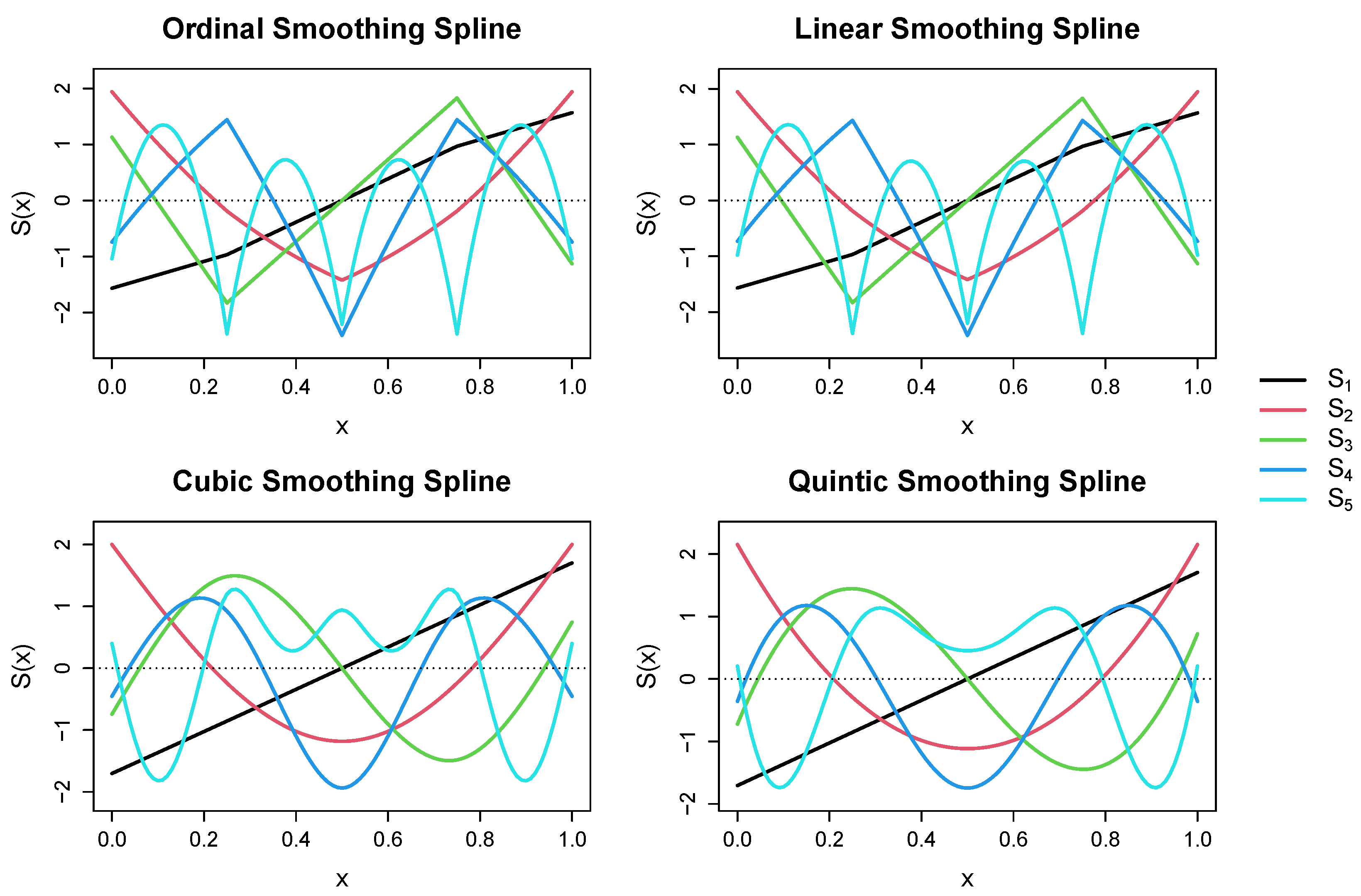
Note that Theorem 4 reveals that modified representation in Theorem 1 can be equivalently expressed in terms of the empirical eigen-decomposition of the penalty matrix, which we refer to as the spectral representation of the smoothing spline. Furthermore, note that the theorem reveals that the spectral basis functions serve as empirical eigenfunctions for , in the sense that these functions are a sample dependent basis that is orthonormal with respect to the contrast space inner-product. These eigenfunctions have the typical sign-changing behavior that is characteristic of spectral representations, such that has more sign changes than for , see Figure 1. Note that the (scaled) ordinal and linear smoothing spline spectra are nearly identical to one another, which is not surprising given the asymptotic equivalence of these kernel functions [28]. Furthermore, note that the (scaled) cubic and quintic smoothing spline spectra are rather similar in appearance, especially for the first four empirical eigenfunctions.

Figure 1.
Spectral basis functions for different types of reproducing kernel functions using five equidistant knots. Basis functions were evaluated at for and were scaled for visualization purposes. Produced by R [29] using the rk() function in the grpnet package [30].
5.2. Tensor Product Formulation
For a more convenient representation of tensor product smoothing spline (like) estimators, I introduce the spectral version of the representer theorem from Theorem 2, which will be particularly useful for tensor product function building.
Theorem 5
(Spectral Tensor Product Representer Theorem). The minimizer of Equation (17) has the form , where is an intercept, and is the k-th effect function for . The optimal effect functions can be expressed as
for all , where is the coefficient vector and are the spectral basis functions for . The spectral basis functions can be defined to satisfy , where is Kronecker’s delta, which implies that for any , where .
Proof.
The result in Theorem 5 is essentially a combination of the results in Theorem 2 and Theorem 4. To prove the result, let denote the vector of RK evaluations at the training data for an arbitrary , and let denote the corresponding penalty matrix. Furthermore, let denote the eigen-decomposition of the penalty matrix, where is the matrix of eigenvectors, and is the diagonal matrix of eigenvalues ( is the i-th singular value). Then the spectral basis functions can be defined as , which ensures that for any . □
Using the spectral tensor products, multiple and generalized nonparametric regression models can be easily fit using standard mixed effects modeling software, such as lme4 [31]. See Figure 2 for a visualization of the spectral tensor product basis functions.
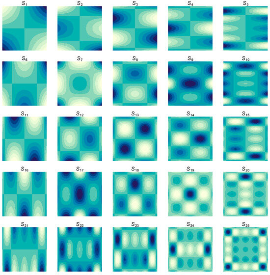
Figure 2.
Spectral tensor product basis functions formed from cubic smoothing spline marginals with equidistant knots for each predictor. From left to right, the basis functions become less smooth with respect to . From top to bottom, the basis functions become less smooth with respect to . Produced by R [29] using the rk() function in the grpnet package [30].
5.3. Scalable Computation
For large n, the spectral basis functions defined in Theorem 5 are not computationally feasible, given that computing the eigen-decomposition of the penalty requires flops. For more scalable computation, I present a spectral version of Corollary 2.
Corollary 3
(Spectral Tensor Product Low-Rank Approximation). The minimizer of Equation (17) has the form , and the effect functions can be approximated via
where is the vector of spectral basis functions corresponding to , which are the selected knots for the k-th effect with .
Using the low-rank approximation, the penalty matrix evaluates the RK function at all combinations of the selected knots . Note that the eigen-decomposition of only requires flops, which is a substantial improvement if . For the main effects, the spectral basis functions can be defined as , where is the eigen-decomposition of the penalty matrix with denoting the ℓ-th eigenvalue/vector pair. As will be demonstrated in the subsequent theorem, spectral basis functions for interaction effects can be defined in a more efficient fashion via the computational tools from Theorem 3.
Theorem 6
(Spectral Tensor Product Penalties). Suppose that and captures the k-th predictor’s main effect for . Given any , the k-th basis vector is defined as and the k-th penalty matrix is , where is the non-constant portion of each predictor’s marginal RK function for . Then the k-th spectral basis vector is defined as , and the corresponding penalty matrix is the identity matrix. Now, suppose that (for some ) captures the interaction effect between and for some . If the basis vector is defined as , where denotes the Kronecker product, then the penalty matrix is the identity matrix. Now, suppose that (for some ) captures the three-way interaction between for some . If the basis vector is defined as , then the penalty matrix is the identity matrix. Basis vectors for higher-order interactions can be efficiently constructed in a similar fashion.
Proof.
To prove the theorem, it suffices to prove the result for two-way interactions, given that three-way (and higher-order) interactions can be built by recursively applying the results from the two-way interaction scenario. Specifically, it suffices to show that the penalty matrix corresponding to is the identity matrix. Letting and denote arbitrary coefficient vectors, the representation for the k-th term is
where the reparameterized basis and coefficient vector can be written as
Now, note that the squared Euclidean norm of the reparameterized coefficients is
where the first line plugs in the definition of the squared Euclidean norm, the second line uses the fact that , the third line uses the fact that , and the fourth line plugs in the definition of the penalty matrices. □
6. Simulated Example
To demonstrate the potential of the proposed approach, I designed a simple simulation study to compare the performance of the proposed tensor product smoothing approach with the approach of Wood et al. [20], which is implemented in the popular gamm4 package [32] in R [29]. The gamm4 package [32] uses the mgcv package [33] to build the smooth basis matrices, and then uses the lme4 package [31] to tune the smoothing parameters (which are treated as variance parameters). For a fair comparison, I have implemented the proposed tensor product spectral smoothing (TPSS) approach using the lme4 package to tune the smoothing parameters, which I refer to as tpss4. This ensures that any difference in the results is due to the employed (reparameterized) basis functions instead of due to differences in the tuning procedure.
Given predictors with , the true mean function is defined as
where is the main effect of the first predictor, and is the main effect of the second predictor. The interaction effect is defined as for the additive function, and for the interaction function. Note that this interaction function has been used in previous simulation work that explored tensor product smoothers (see [9,34]). Two different sample sizes were considered . For each sample size and data-generating mean function, n observations were (independently) randomly sampled from , and the response was defined as , where follows a standard normal distribution.
For both the gamm4 package and the proposed tpss4 implementation, (i) I fit the model using marginal knots for each predictor, and (ii) I used restricted maximum likelihood (REML) to tune the smoothing parameters. For the gamm4 package, the tensor product smooth was formed using the t2() function, which allows for main and interaction effects of the predictors. For the tpss4 method, the implementation in the smooth2d() function (see Supplementary Materials) allows for both main and interaction effects. Thus, for both methods, the fit model is misspecified for additive models and correctly specified for interaction models.
I compared the quality of the solutions using the root mean squared error (RMSE)
and the mean absolute error (MAE)
where is the data-generating mean function and is the estimated function. The data generation and analysis procedure was repeated 100 times for each sample size.
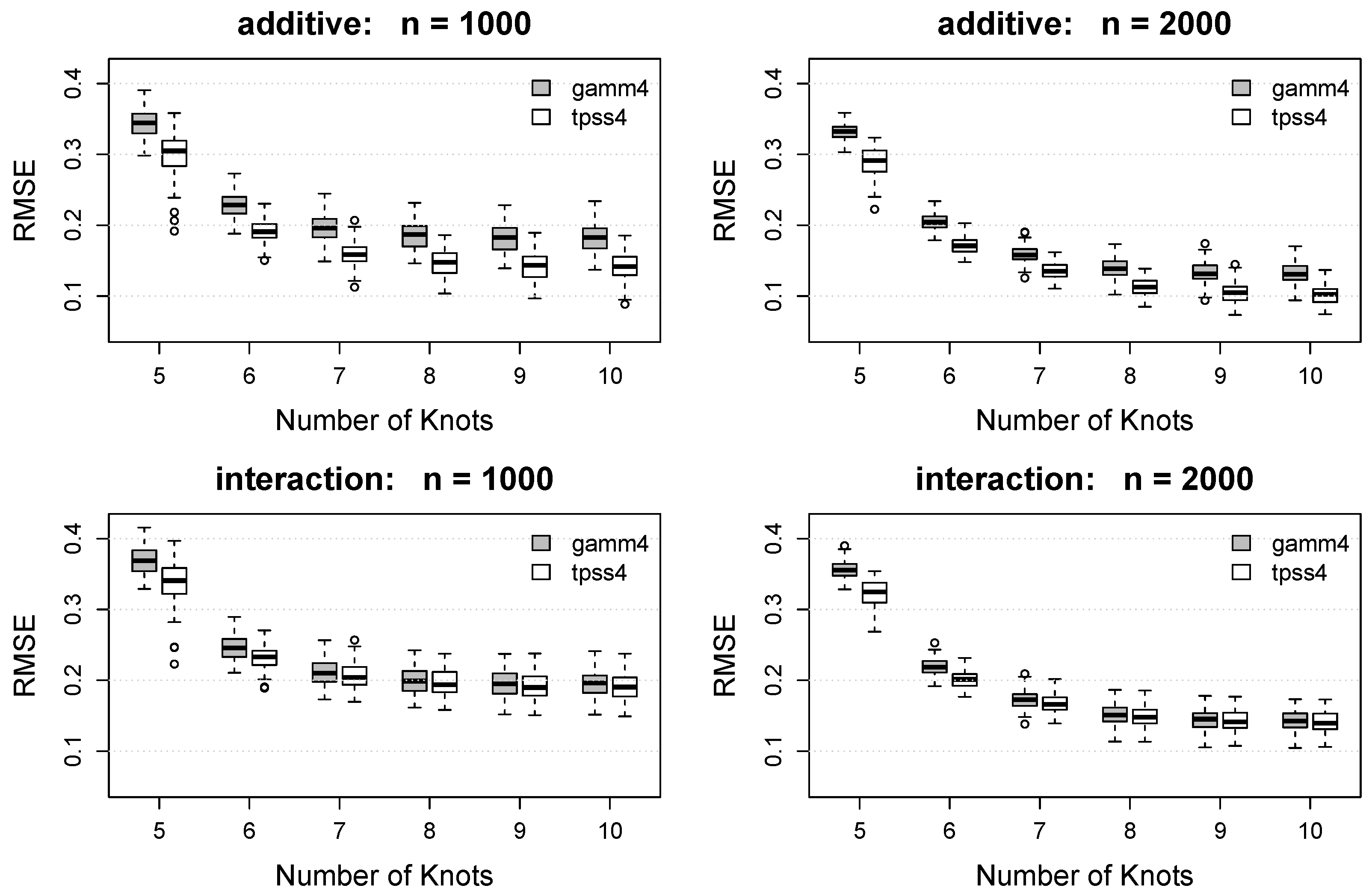
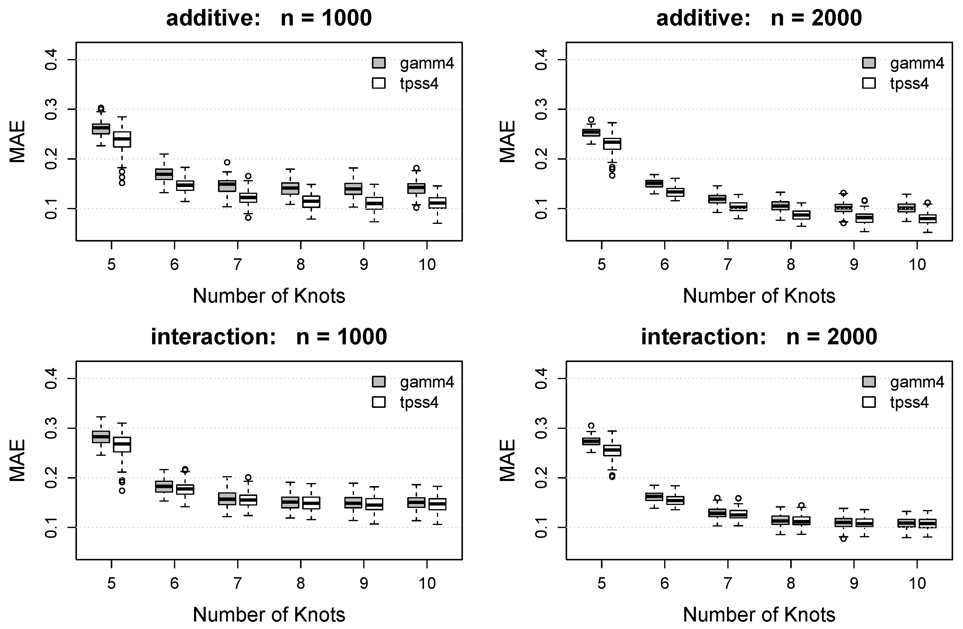
Box plots of the RMSE and MAE for each method under each combination of and are displayed in Figure 3 and Figure 4. As expected, both the RMSE and MAE decrease as the number of knots increases for both methods. For each , the proposed tpss4 method tends to result in smaller RMSE and MAE values compared to the gamm4 implementation. For the (misspecified) additive function, the benefit of the proposed approach is noteworthy and persists across all . For the interaction model, the benefit of the proposed tpss4 approach is particularly noticeable for small , but is still existent for larger numbers of knots.
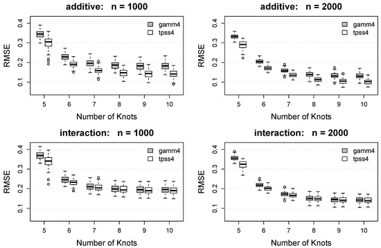
Figure 3.
Box plots of the root mean squared error (RMSE) of the function estimate for each method. Rows show results for the additive function (top) and interaction function (bottom). Columns show the results as a function of the number of knots for (left) and (right). Gray boxes denote the results using the gamm4 packages, whereas white boxes denote the results using the proposed tpss4 approach. Each box plot summarizes the results across the 100 simulation replications.
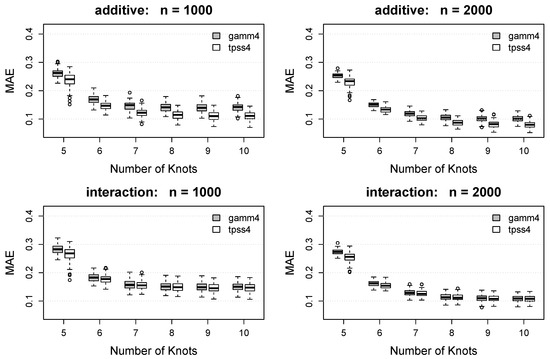
Figure 4.
Box plots of the mean absolute error (MAE) of the function estimate for each method. Rows show results for the additive function (top) and interaction function (bottom). Columns show the results as a function of the number of knots for (left) and (right). Gray boxes denote the results using the gamm4 packages, whereas white boxes denote the results using the proposed tpss4 approach. Each box plot summarizes the results across the 100 simulation replications.
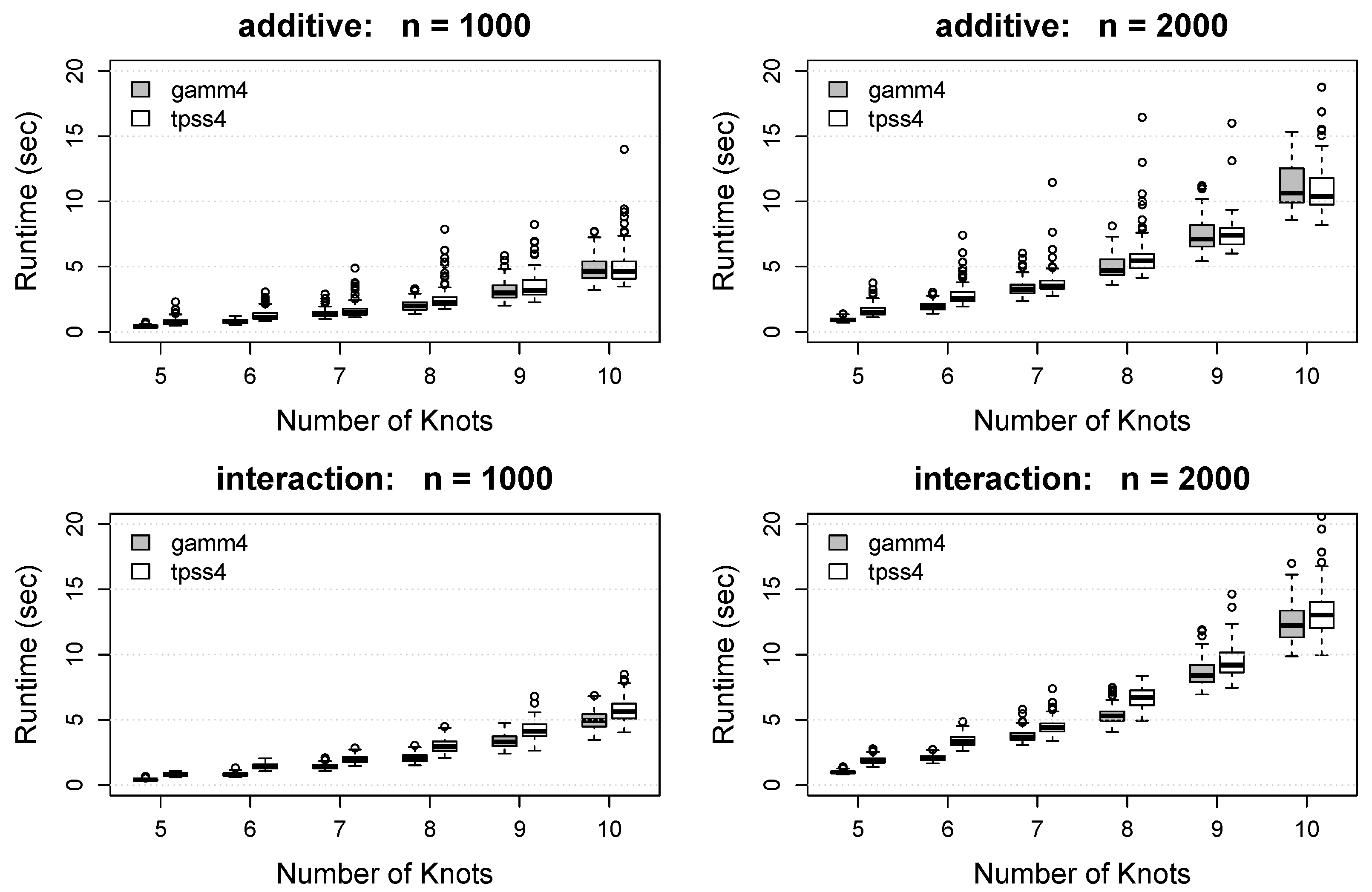
The runtime for each method is displayed in Figure 5. The proposed tpss4 method produces runtimes that are slightly larger than the gamm4 method in most situations. Despite using the same number of marginal knots for each predictor, the gamm4 approach uses an approximation that estimates slightly fewer coefficients, which is likely causing the timing differences. However, it is possible that these timing differences could be due to running compiled code (in gamm4) versus uncompiled code (in tpss4). Regardless of the source of the differences, the timing differences are rather small and disappear as increases, which reveals the practicality of the proposed approach.

Figure 5.
Box plots of the algorithm runtime (in seconds) for each method. Rows show results for the additive function (top) and interaction function (bottom). Columns show the results as a function of the number of knots for (left) and (right). Gray boxes denote the results using the gamm4 packages, whereas white boxes denote the results using the proposed tpss4 approach. Each box plot summarizes the results across the 100 simulation replications.
7. Real Data Example
To demonstrate the proposed approach using real data, I make use of the Bike Sharing Dataset [35] from the UCI Machine Learning Repository [36]. This dataset contains the number (count) of bikes rented from the Capital Bike Share system in Washington DC. The rental counts are recorded by the hour from the years 2011 and 2012, which produced a dataset with n = 17,379 observations. In addition to the counts, the dataset contains various situational factors that might affect the number of rented bikes. In this example, I will focus on modeling the number of bike rentals as a function of the hour of the day (which takes values 0, 1, …, 23) and the month of the year (which takes values 1, 2, …, 12).
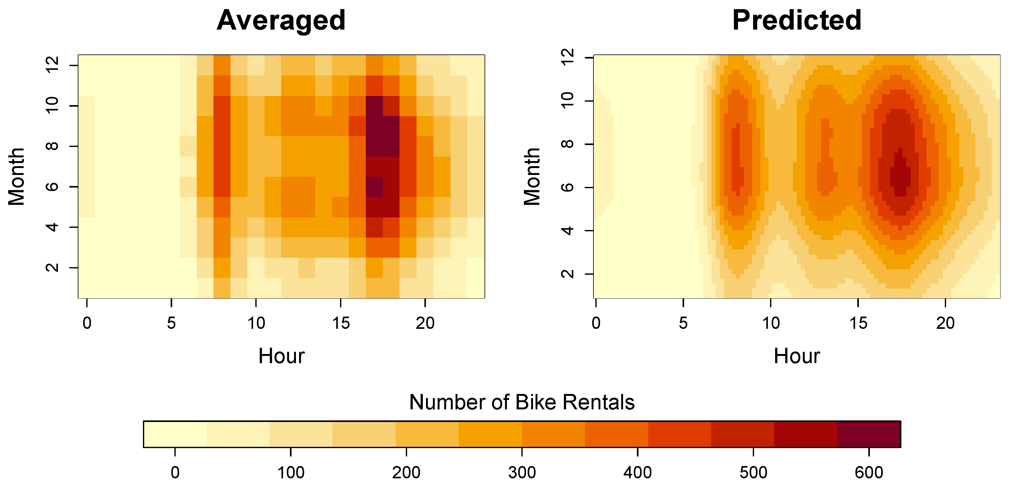
The proposed approach was used to fit a tensor product spectral smoother (TPSS) to the data using 12 knots for the hour variable and 6 knots for the month variable. The counts were modeled on the log10 scale, and then transformed back to the original (data) scale for visualization purposes. As in the simulation study, the smoothing parameters were tuned using the REML method in the lme4 package. Figure 6 displays the average number of bike rentals by hour and month, as well as the TPSS model predictions. As is evident from the figure, the TPSS solution closely resembles the average data; however, the model predictions are substantially smoother, which improves the interpretation.

Figure 6.
Real data results. (left) average number of bike rentals by hour and month. (right) predicted number of bike rentals by hour and month.
Looking at the bike rental patterns by hour of the day, it is evident that there are two surges in the number of rentals: (1) during the morning rush hour (∼8:00–9:00) and (2) during the evening rush hour (∼17:00–18:00). The results also reveal another (smaller) surge that occurs during the lunch hour (∼12:00–13:00). Interestingly, the predictions in Figure 6 reveal that the bike rental surge during the morning rush hour is more localized in time (lasting about one hour), whereas the evening surge is more temporally diffuse (lasting 2–3 h). The bike rentals tend to peak during the afternoon rush hour, and are at their lowest expected value during the evening hours (∼23:00–06:00).
The month effect is less pronounced than the hour effect, but it still produces some interpretable insights. In particular, we see that there are fewer people using the bikes during the winter months (Dec, Jan, Feb), which is expected. The drops in the number of rentals during the winter are particularly noticeable during the lunch surge, which suggests that fewer people use the bikes to compute for lunch during the winter. The peak in the rentals occurs during the summer months (Jun, Jul, Aug). Combining the hour and month information suggests that the evening rush hour during the summer months is when the Capital Bike Share system sees it greatest surge in demand.
8. Discussion
This paper proposes efficient and flexible approaches for fitting tensor product smoothing spline-like models. The refined smoothing spline approach developed in Section 4 offers an alternative approach for tensor product smoothing splines that penalizes all non-constant effects of the predictors. In particular, Theorem 1 proposes a representer theorem for univariate smoothing spline-like estimators that penalizes all non-constant functions, Theorem 2 provides a tensor product extension of the proposed estimator, and Theorem 3 develops efficient computational tools for forming tensor product penalties. Furthermore, the spectral tensor product approach developed in Section 5 makes it possible to use exact (instead of approximate) tensor product penalties, which can be easily implemented in any standard mixed effects modeling software. In particular, Theorem 4 presents a spectral representer theorem for univariate smoothing, Theorem 5 provides a tensor product extension of the spectral representation, and Theorem 6 develops efficient computational tools for forming tensor product penalties.
The principal results in this paper reveal that if basis functions are formed by taking Kronecker products of spectral spline representations, then the resulting (exact) penalty matrix is the identity matrix. This implies that it is no longer necessary to choose between approximate penalties or costly parameterizations. Note that the results in this paper provide some theoretical support for the tensor product approach of Wood et al. [20], which uses a similar approach with different basis functions. The simulation results support the theoretical results given that the proposed approach (which uses the exact penalty) outperforms the approach of Wood et al. [20] in gamm4 [32]. As a result, I expect that the proposed approach will be quite useful for fitting (generalized) nonparametric models using modern mixed effects and penalized regression modeling softwares such as lme4 or grpnet. Furthermore, I expect that the proposed approach will be useful for conducting inference with tensor product smoothing splines, e.g., using nonparametric permutation tests [37] or standard hypothesis tests for variance components [38].
Supplementary Materials
The following supporting information can be downloaded at: https://www.mdpi.com/2571-905X/7/1/3/s1.
| Name | Type | Description |
| smooth2d | R function (.R) | Function for 2-dimensional smoothing |
| tpss_ex | R script (.R) | Script for the bike sharing analyses and Figure 6 |
| tpss_figs | R script (.R) | Script for reproducing Figure 1 and Figure 2 |
| tpss_sim | R script (.R) | Script for the simulation study and Figure 3, Figure 4 and Figure 5 |
Funding
This research was funded by National Institutes of Health (NIH) grants R01EY030890, U01DA046413, and R01MH115046.
Institutional Review Board Statement
Not applicable.
Informed Consent Statement
Not applicable.
Data Availability Statement
R code to reproduce the results is included as Supplementary Materials. The analyzed data are open source and publicly available.
Conflicts of Interest
The author declares no conflict of interest.
References
- Helwig, N.E. Multiple and Generalized Nonparametric Regression. In SAGE Research Methods Foundations; Atkinson, P., Delamont, S., Cernat, A., Sakshaug, J.W., Williams, R.A., Eds.; SAGE Publications Ltd.: London, UK, 2020. [Google Scholar] [CrossRef]
- Berry, L.N.; Helwig, N.E. Cross-validation, information theory, or maximum likelihood? A comparison of tuning methods for penalized splines. Stats 2021, 4, 701–724. [Google Scholar] [CrossRef]
- Wahba, G. Spline Models for Observational Data; Society for Industrial and Applied Mathematics: Philadelphia, PA, USA, 1990. [Google Scholar]
- de Boor, C. A Practical Guide to Splines; revised ed.; Springer: New York, NY, USA, 2001. [Google Scholar]
- Gu, C. Smoothing Spline ANOVA Models, 2nd ed.; Springer: New York, NY, USA, 2013. [Google Scholar] [CrossRef]
- Wang, Y. Smoothing Splines: Methods and Applications; CRC Press: Boca Raton, FL, USA, 2011. [Google Scholar]
- Wood, S.N. Generalized Additive Models: An Introduction with R, 2nd ed.; Chapman & Hall: Boca Raton, FL, USA, 2017. [Google Scholar]
- Hastie, T.; Tibshirani, R. Generalized Additive Models; Chapman and Hall/CRC: New York, NY, USA, 1990. [Google Scholar]
- Helwig, N.E.; Ma, P. Fast and stable multiple smoothing parameter selection in smoothing spline analysis of variance models with large samples. J. Comput. Graph. Stat. 2015, 24, 715–732. [Google Scholar] [CrossRef]
- Helwig, N.E.; Gao, Y.; Wang, S.; Ma, P. Analyzing spatiotemporal trends in social media data via smoothing spline analysis of variance. Spat. Stat. 2015, 14, 491–504. [Google Scholar] [CrossRef]
- Helwig, N.E.; Shorter, K.A.; Hsiao-Wecksler, E.T.; Ma, P. Smoothing spline analysis of variance models: A new tool for the analysis of cyclic biomechaniacal data. J. Biomech. 2016, 49, 3216–3222. [Google Scholar] [CrossRef] [PubMed]
- Helwig, N.E.; Ruprecht, M.R. Age, gender, and self-esteem: A sociocultural look through a nonparametric lens. Arch. Sci. Psychol. 2017, 5, 19–31. [Google Scholar] [CrossRef]
- Helwig, N.E.; Sohre, N.E.; Ruprecht, M.R.; Guy, S.J.; Lyford-Pike, S. Dynamic properties of successful smiles. PLoS ONE 2017, 12, e0179708. [Google Scholar] [CrossRef]
- Helwig, N.E.; Snodgress, M.A. Exploring individual and group differences in latent brain networks using cross-validated simultaneous component analysis. NeuroImage 2019, 201, 116019. [Google Scholar] [CrossRef] [PubMed]
- Hammell, A.E.; Helwig, N.E.; Kaczkurkin, A.N.; Sponheim, S.R.; Lissek, S. The temporal course of over-generalized conditioned threat expectancies in posttraumatic stress disorder. Behav. Res. Ther. 2020, 124, 103513. [Google Scholar] [CrossRef]
- Almquist, Z.W.; Helwig, N.E.; You, Y. Connecting Continuum of Care point-in-time homeless counts to United States Census areal units. Math. Popul. Stud. 2020, 27, 46–58. [Google Scholar] [CrossRef]
- Helwig, N.E. Efficient estimation of variance components in nonparametric mixed-effects models with large samples. Stat. Comput. 2016, 26, 1319–1336. [Google Scholar] [CrossRef]
- Helwig, N.E.; Ma, P. Smoothing spline ANOVA for super-large samples: Scalable computation via rounding parameters. Stat. Its Interface 2016, 9, 433–444. [Google Scholar] [CrossRef]
- Demmler, A.; Reinsch, C. Oscillation matrices with spline smoothing. Numer. Math. 1975, 24, 375–382. [Google Scholar] [CrossRef]
- Wood, S.N.; Scheipl, F.; Faraway, J.J. Straightforward intermediate rank tensor product smoothing in mixed models. Stat. Comput. 2013, 23, 341–360. [Google Scholar] [CrossRef]
- Kimeldorf, G.; Wahba, G. Some results on Tchebycheffian spline functions. J. Math. Anal. Appl. 1971, 33, 82–95. [Google Scholar] [CrossRef]
- Gu, C.; Kim, Y.J. Penalized likelihood regression: General formulation and efficient approximation. Can. J. Stat. 2002, 30, 619–628. [Google Scholar] [CrossRef]
- Kim, Y.J.; Gu, C. Smoothing spline Gaussian regression: More scalable computation via efficient approximation. J. R. Stat. Soc. Ser. B 2004, 66, 337–356. [Google Scholar] [CrossRef]
- Moore, E.H. On the reciprocal of the general algebraic matrix. Bull. Am. Math. Soc. 1920, 26, 394–395. [Google Scholar] [CrossRef]
- Penrose, R. A generalized inverse for matrices. Math. Proc. Camb. Philos. Soc. 1955, 51, 406–413. [Google Scholar] [CrossRef]
- Wang, Y. Mixed effects smoothing spline analysis of variance. J. R. Stat. Soc. Ser. B 1998, 60, 159–174. [Google Scholar] [CrossRef]
- Wang, Y. Smoothing spline models with correlated random errors. J. Am. Stat. Assoc. 1998, 93, 341–348. [Google Scholar] [CrossRef]
- Helwig, N.E. Regression with ordered predictors via ordinal smoothing splines. Front. Appl. Math. Stat. 2017, 3, 15. [Google Scholar] [CrossRef]
- R Core Team. R: A Language and Environment for Statistical Computing; R Foundation for Statistical Computing: Vienna, Austria, 2023; R version 4.3.1. [Google Scholar]
- Helwig, N.E. grpnet: Group Elastic Net Regularized GLM, R package version 0.2; Comprehensive R Archive Network: Vienna, Austria, 2023. [Google Scholar]
- Bates, D.; Mächler, M.; Bolker, B.M.; Walker, S.C. Fitting Linear Mixed-Effects Models Using lme4. J. Stat. Softw. 2015, 67, 1–48. [Google Scholar] [CrossRef]
- Wood, S.; Scheipl, F. gamm4: Generalized Additive Mixed Models Using ‘mgcv’ and ‘lme4’, R package version 0.2-6; Comprehensive R Archive Network: Vienna, Austria, 2020. [Google Scholar]
- Wood, S.N. mgcv: Mixed GAM Computation Vehicle with GCV/AIC/REML Smoothness Estimation and GAMMs by REML/PQL, R package version 1.9-1; Comprehensive R Archive Network: Vienna, Austria, 2023. [Google Scholar]
- Helwig, N.E. Spectrally sparse nonparametric regression via elastic net regularized smoothers. J. Comput. Graph. Stat. 2021, 30, 182–191. [Google Scholar] [CrossRef]
- Fanaee-T, H.; Gama, J. Event labeling combining ensemble detectors and background knowledge. Prog. Artif. Intell. 2013, 2, 1–15. [Google Scholar] [CrossRef]
- Kelly, M.; Longjohn, R.; Nottingham, K. The University of California Irvine (UCI) Machine Learning Repository. Available online: https://archive.ics.uci.edu/ (accessed on 26 December 2023).
- Helwig, N.E. Robust Permutation Tests for Penalized Splines. Stats 2022, 5, 916–933. [Google Scholar] [CrossRef]
- Kuznetsova, A.; Brockhoff, P.B.; Christensen, R.H.B. lmerTest Package: Tests in Linear Mixed Effects Models. J. Stat. Softw. 2017, 82, 1–26. [Google Scholar] [CrossRef]

Disclaimer/Publisher’s Note: The statements, opinions and data contained in all publications are solely those of the individual author(s) and contributor(s) and not of MDPI and/or the editor(s). MDPI and/or the editor(s) disclaim responsibility for any injury to people or property resulting from any ideas, methods, instructions or products referred to in the content. |
© 2024 by the author. Licensee MDPI, Basel, Switzerland. This article is an open access article distributed under the terms and conditions of the Creative Commons Attribution (CC BY) license (https://creativecommons.org/licenses/by/4.0/).