Article

Active Learning for Stacking and AdaBoost-Related Models

Department of Statistics, North Carolina State University, 2311 Stinson Dr, Raleigh, NC 27695-8203, USA
*
Author to whom correspondence should be addressed.
Stats 2024, 7(1), 110-137; https://doi.org/10.3390/stats7010008
Submission received: 12 December 2023 / Revised: 15 January 2024 / Accepted: 22 January 2024 / Published: 24 January 2024

Abstract

:
Ensemble learning (EL) has become an essential technique in machine learning that can significantly enhance the predictive performance of basic models, but it also comes with an increased cost of computation. The primary goal of the proposed approach is to present a general integrative framework that allows for applying active learning (AL) which makes use of only limited budget by selecting optimal instances to achieve comparable predictive performance within the context of ensemble learning. The proposed framework is based on two distinct approaches: (i) AL is implemented following a full scale EL, which we call the ensemble learning on top of active learning (ELTAL), and (ii) apply the AL while using the EL, which we call the active learning during ensemble learning (ALDEL). Various algorithms for ELTAL and ALDEL are presented using Stacking and Boosting with various algorithm-specific query strategies. The proposed active learning algorithms are numerically illustrated with the Support Vector Machine (SVM) model using simulated data and two real-world applications, evaluating their accuracy when only a small number instances are selected as compared to using full data. Our findings demonstrate that: (i) the accuracy of a boosting or stacking model, using the same uncertainty sampling, is higher than that of the SVM model, highlighting the strength of EL; (ii) AL can enable the stacking model to achieve comparable accuracy to the SVM model using the full dataset, with only a small fraction of carefully selected instances, illustrating the strength of active learning.

1. Introduction

Basic machine learning models may not always be capable of achieving the desired level of performance. Following are some examples: (i) Certain models may excel in capturing specific features, while others may perform better in other feature domains; (ii) When only a limited number of training instances are available, the effectiveness of traditional machine learning models can be severely constrained; (iii) When faced with complex decision boundaries or data patterns that cannot be effectively modeled by a single model, ensemble techniques and other more sophisticated machine learning approaches may be required.
An illustration of such a scenario is presented in Figure 1, where a total of 26 instances to be used in the training phase are shown in blue. Each instance is characterized by a pair of covariates and belongs to one of three different classes, represented by distinctive shapes such as circles, squares, and triangles. To explore the impact of training set selection on the performance of machine learning models, three separate training sets were generated by randomly drawing 12 instances from the pool of 26 for use training a model. The selected instances in each subfigure were identified and color-coded as magenta, yellow, and green, respectively. The trained models utilized these instances to develop individual hypotheses, each of which is depicted using the corresponding color. While these hypotheses are generally effective in predicting the classes of the instances, none provides a complete and accurate characterization of the underlying decision boundary. On the other hand, by combining all three hypotheses using an averaging approach, the resulting ensembled hypothesis is able to reduce the variances inherited from the basic learners effectively.
In the machine learning field, classification models of the same or different types could be put together to build a more powerful model. This approach is referred to as ensemble learning. In essence, Ensemble Learning (EL) aims to improve the performance and robustness of a model by combining the predictions of multiple base models. EL is often employed when dealing with complex datasets or to enhance the generalization ability of models.
Several studies have investigated the strengths and limitations of ensemble learning. Notable benefits of ensemble learning include improved predictive accuracy, reduced variance and bias for the estimated parameters [1]. Ensemble learning can leverage the unique strengths of different model types to develop a more comprehensive understanding of the underlying data patterns. However, the results of this approach can be challenging to interpret as it may be difficult to calibrate the individual parameters from multiple models. Additionally, ensemble learning can be computationally expensive in terms of time and operational cost in practice.
Although EL is a well developed field of research, for completeness, we provide a quick glimpse of the EL methods. Traditional ensemble learning approaches fall into two categories: Sequential and Parallel. As for sequential ensemble methods, basic learners are dependent on the results from the previous ones. AdaBoost [2,3,4,5] and its boosting-related variants are some of the most popular sequential ensemble methods. In Boosting, the subsequent basic model corrects the error made by its predecessor. Weights of previously mislabeled examples are increased and weights of previously correctly labeled examples are decreased. On the other hand, there is no interdependence among the basic learners in parallel ensemble learning techniques. Multiple models can be trained concurrently and separately. To obtain the final estimation, further integration must be chosen to merge the hypotheses produced by each learner. For classification problems, if each basic learner’s decision regarding an instance’s class falls within the range of 0 and 1, possible integration mechanisms include the mean, weighted average, or the product of the decisions. In addition to using a function based on those basic decisions, the integration rule could also be learned via an additional machine learning model. Since different machine learning models are stacked on different levels, this technique is referred to as stacking [6,7].
Regardless of the specific updates applied to subsequent learners in Boosting or the particular integration techniques chosen in parallel approaches, ensemble learning models inevitably incur additional computational burden. Moreover, in situations where there are constraints on the resources available for labeling, but where the benefits of ensemble learning models are still desirable, the active learning framework can offer a viable solution. The primary focus of Active Learning (AL) is on reducing the amount of labeled data needed for training by intelligently selecting the most informative instances for labeling. AL is beneficial when labeling data is expensive or time-consuming. It is often used in scenarios where there is a large pool of unlabeled data, and the model is allowed to query the most valuable instances for labeling.
The majority of active learning approaches, including random sampling, uncertainty sampling [8,9], and expected error reduction (EER) [10], adopt a model-free approach in which instances are selected based on predicted probabilities or data structure. As a consequence, active learning algorithms are not limited to simple logistic regression models and can be applied to a diverse range of more complex models, including deep neural networks [11], classification trees, and gradient boosting machines [5].
Recent years have witnessed a growing interest in leveraging Active Learning (AL) in the context of deep learning models, particularly owing to the remarkable performance of these models on complicated tasks [12,13]. A variety of techniques have been proposed that combine deep learning and active learning, including Deep Bayesian Active Learning (DBAL) [14], uncertainty estimates using deep ensembles [15], geometry-based approaches [16], and Deep Ensemble Bayesian Active Learning (DEBAL) [17].
Despite extensive research for EL and AL for basic learners and convolutional neural networks, the topic of integrating AL within the EL has largely remained unexplored. Specifically, this study focuses on active learning techniques in the context of Boosting and Stacking. While ensemble learning aims to combine multiple hypotheses using a fixed dataset, active learning involves sequentially selecting instances from the pool. A crucial question that arises pertains to the timing of instance selection. When the training data is updated during ensemble learning, it is not clear whether the learners can still be improved. In our proposed work, this scenario will be referred to as active learning during ensemble learning (ALDEL). Conversely, if instance selection is performed after the integration of basic learners, the efficiency of active learning may be limited. This scenario will be referred to as ensemble learning on top of active learning (ELTAL).
Figure 2 highlights the mechanism of shifting from active learning in basic models to active ensemble learning, with a particular emphasis on classification problems. The red parts in Figure 2 denote the key aspects of this study.
To the best of our knowledge, we provide the first general framework for integrating active learning within ensemble learning. Our exposition is specifically for AdaBoost-related and Stacking-related models. We consider the ELTAL and ALDEL cases separately for both models and propose four different general algorithms, one for each setting in detail. For ELTAL algorithms, we apply active learning query strategies directly to the ensemble learner. For ALDEL in Boosting, we select instances that maximize the exponential loss and present them to the oracle for labeling. After labeling, we assign a pseudo weight to these instances for use in subsequent iterations. For ALDEL in Stacking, we divide query strategies into two categories: two-level selection and direct selection. In two-level selection, each lower-level model independently selects a candidate based on its own criterion. A second-level algorithm then chooses the final instance from these candidates. In direct selection, we treat the lower-level model’s output as a transformation from the input space to a range between 0 and 1. This probabilistic output, which is more informative than raw input data, is then subjected to traditional active learning algorithms.
The structure of this article is outlined as below: In Section 2, we present a brief review of the sequential and parallel ensemble learning approaches. In Section 3, we provide a general overview of active learning, the challenges and key points of combining active learning with ensemble learning. In Section 4 and Section 5, we introduce our proposed active learning technique in AdaBoost-related and stacking models, respectively. In Section 6, we numerically illustrate the performance of different ensemble active learning algorithms using simulated datasets and real-world applications. In Section 7, we conclude this article by discussing the strength and weaknesses of our work.

2. Ensemble Learning: A Brief Review

Suppose a set of possibly vector valued observations x 1 , x 2 , , x n arise independently from a distribution D X . Let y 1 , y 2 , , y n { 1 , + 1 } denote the corresponding labels. We assume that the pairs ( x i , y i ) , i = 1 , 2 , , n arise independently from a joint distribution D X Y . Denote the collection of different active learning criteria such as uncertainty sampling [8], expected error reduction [10] as A . The hypotheses come from the set of mappings, H : D X { 1 , + 1 } . We use the function err to denote the training error of a classifier h based on full sample S n = { ( x 1 , y 1 ) , ( x 2 , y 2 ) , , ( x n , y n ) } , i.e.,
err S n ( h ) = 1 n i = 1 n 1 { h ( x i ) y i }
Denote the ground truth classifier as h 0 H , such that h 0 ( x ) = y , x , y D X Y . In other words, err S n ( h 0 ) = 0 .
Following the same setting as typically used for Probably Approximately Correct (PAC) learning [18], we define the concepts of weak learning and strong learning. A strong learner could attain arbitrarily low error as long as enough instances are provided. For any given ϵ > 0 and δ < 1 2 , a strong learner would return a classifier h such that
Pr { err S n ( h ) < 1 2 ϵ } > 1 δ
with n = Poly ( 1 ϵ , 1 δ , VCDim ( H ) ) instances, where VCDim ( H ) denotes the VC dimension of H . A weak learning algorithm output a classifier h that performs better than random guessing. In other words, there exists ϵ 0 > 0 and δ 0 < 1 2 , such that (1) holds.
Generally speaking, the weakness of a learning algorithm is associated with the magnitude of bias or variance. The core of ensemble learning is to convert a weak learner to a strong learner by reducing either the biases or the variances of the weak learner.

2.1. Boosting

The core idea of boosting-type methods is combining different learners, where the next learner corrects the previous learner’s error. The first boosting algorithm was proposed by [19]. It provides three classifiers, where the second classifier is trained with a sample that includes at least half of the misclassified samples by the first learner. The third learner is trained on the instances in which the first two learners disagree. The most famous boosting algorithm is AdaBoost [2,3,4,5], which is presented in Algorithm 1. Here, we use M as the number of basic classifiers used for boosting. In other words, the algorithm is halted after M iterations. The choice of M depends on the early stopping of a boosting algorithm. As larger M may lead to larger variances, numerous studies, such as [20], suggest that selecting a large M may result in overfitting. Therefore, M should be chosen to ensure the algorithm converges, as noted in [21]. Practically, this parameter is often determined by data-derived early stopping rules and empirical testing. In Algorithm 1, M is treated as an input parameter, whereas in parallel ensembling techniques that are introduced in the following Sections, M is automatically determined by the number of parallel basic learners selected by the user.
Algorithm 1 AdaBoost Algorithm
Stats 07 00008 i001
In order to keep the weight α m as positive, the error for the classifier at each iteration can not exceed 0.5. This matches the assumption that the learner to be boosted by the algorithm should be a weak learner.
Theorem 1
([4], Theorem 6). If the m-th hypothesis is better than a random guessing by γ m , i.e., err S n ( h m ) = 1 2 γ m , then
err S n ( H ) exp ( 2 m = 1 M γ m 2 )
If γ m ’s are bounded below by γ , the upper bound of (2) could be replaced by exp ( 2 M γ 2 ) . Another theorem has shown that the upper bound could be replaced by 2 M m = 1 M ( 1 2 γ m ) ( 1 2 + γ m ) . With the assumption that all γ m ’s are less than 1 2 . the AdaBoost procedure has enabled the outputted hypothesis to attain arbitrarily low training error with sufficient instances. Other than training error, the generalization error of the outputted hypothesis could also be bounded from above.
Theorem 2
([4], Theorem 7). With high probability, the generalization error of the outputted hypothesis could be bounded as
err D X Y ( H ) err S n ( H ) + O ˜ ( M · VCDim ( H ) n )
Following the same idea of boosting, some variants are proposed. In Discrete Adaboost, the output of each hypothesis is binary as either 1 or 1. Schapire and Singer [22] introduced a generalized version of AdaBoost such that the output of the hypothesis could be real-valued instead of being restricted in [ 1 , 1 ] . Friedman et al. [23] viewed the AdaBoost-related procedure as fitting an additive model to a target function. Denote the exponential loss function as
J ( H ) = E [ e y H ( x ) ] , y { 1 , + 1 } .
Specifically, Friedman et al. [23] demonstrated that Boosting can be viewed as minimizing the Equation (4) by constructing an additive model aimed at 1 2 log Pr ( y = 1 | x ) Pr ( y = 1 | x ) , which is the minimizer of J ( H ) . With an existing ensemble hypothesis H, the update process at each iteration involves minimizing J ( H + α h ) in the subsequent iteration, w.r.t α and h. If the output of each hypothesis could be real-valued confidence, Equation (4) could be minimized by directly setting the derivative J / h as 0. This becomes the update rule from the other algorithm Real AdaBoost proposed by Friedman et al. [23]. In Discrete AdaBoost, however, the optimization step are restricted under the condition that the output of h is binary. Friedman et al. [23] further demonstrated that the expected value of the negative log-likelihood function, after transforming the responses of the negative class instances from 1 to 0, shares the same minimizer as J ( H ) . This insight led to the development of the LogitBoost and Gentle AdaBoost algorithms. Both aim to enhance the current ensemble hypothesis by employing a Newton step to minimize the expected negative log-likelihood and J ( H ) , respectively, at each iteration.

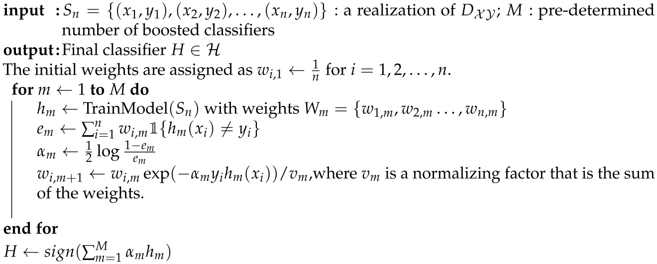
2.2. Parallel Ensemble Learning

Suppose we have a set of hypotheses h 1 , h 2 , , h M H . Each of them is outputted by a single basic learner on S n . In parallel ensemble learning, hypotheses could come from different types of models. Given an instance x, we denote that the support that it belongs to the positive class from the m-th hypothesis as h m ( x ) [ 0 , 1 ] , m = 1 , 2 , , M , then the predicted label for x is taken as the maximizer of the ensembled decision d ( x ) . The generalized mean rule of a decision function is given as    
d ( x | h 1 , h 2 , , h M ) = 1 M m = 1 M w m ( h m ( x ) ) α 1 / α , m = 1 M w m = 1 .
Some special cases from this rule include: (i) α = 1 and w m = 1 / m , m leads to the mean rule; (ii) α = 1 and w m ’s not identical leads to the weighted mean rule; (iii) α 0 and w m = 1 / m , m leads to the product rule; (iv) w m = 1 / m , m and α leads to the maximum rule [24].
An alternative to using a single function to aggregate results from multiple classifiers is to construct a new machine learning model that learns the optimal combination rule. This approach allows for a more systematic and data-oriented fusion of information from multiple models. Wolpert [6] proposed a stacked generalization framework, which combined cross-validation with the training of multiple classifiers. More specifically, suppose we use a K-fold cross-validation. S n is partitioned into K disjoint subsets S n ( 1 ) , S n ( 2 ) , …, S n ( K ) with roughly equal sizes. Denote S ¯ n ( k ) = S n S n ( k ) . During the training phase, each machine learning model h m ( k ) is trained on S ¯ n ( k ) , k = 1 , 2 , , K and predicted on S n ( k ) . Denote z i m = h m ( k ) ( x i ) , m = 1 , 2 , , M if x i S n ( k ) and let z i = ( z i 1 , z i 2 , , z i M ) . As predictions from M machine learning models, z i ’s are treated as intermediate covariates to learn the combination rule and we call them level-1 data. Denote C V n ( k ) = { ( z i , y i ) | x i S n ( k ) } as the collection of level-1 data along with their labels for the k-th cross-validation set. Another machine learning model H is further trained on C V n = k = 1 K C V n ( k ) . Here the basic models h 1 , h 2 , , h M are also referred to as lower-level learners, while H is regarded as the upper-level learner. If all models are trained on the same original dataset S n , they are likely to be highly correlated. The cross-validation procedure effectively prevents overfitting.
We use Figure 3 to visualize a typical stack learning model. Suppose we use a three-fold cross-validation on four lower-level models M 1 , M 2 , M 3 and M 4 . After partitioning, S n ( 1 ) , S n ( 2 ) and S n ( 3 ) are passed to all models on the lower-levels. The predictions on the k-th fold C V n ( k ) are combined from h 1 ( k ) , h 2 ( k ) , h 3 ( k ) and h 4 ( k ) . The intermediate covariates are then vertically concatenated as C V n to feed H.
After the proposal of stacked generalization in [6], Breiman [7] discussed its eligibility in regression models and illustrated with some simulation examples. As another combining strategy, Another approach, Bayes Model Averaging (BMA), assigns weights to different learners based on their posterior probabilities, a method investigated in studies by [25,26,27]. Clarke [28] has demonstrated that BMA is not worse than stacking under the assumption that the correct data generating model (DGM) is on the list of models under consideration and the bias is relatively low. However, this scenario is too idealistic in practice. Generally, stacking is more robust and superior to BMA [29].
Ensemble learning, while powerful, faces challenges with increasing computational demands due to the necessity of training and integrating multiple models. The first challenge lies in the training of multiple models; this process can be particularly time-intensive for complex models or when dealing with large datasets. Additionally, combining the outputs of these models further escalates computational requirements. For instance, in AdaBoost algorithms, recalculating weights for all instances in each iteration and deriving the final prediction from a weighted average of all model predictions adds to the computational load. In parallel ensemble learning methods, the integration of support from each lower-level model through a decision function also increases computational complexity. This complexity is further amplified in stacking-based approaches, where an upper-level model must be trained to learn the combination rule, adding to the training burden. This motivates us to leverage active learning from traditional machine learning models to ensemble learning models, which can substantially reduce the labeling and computational cost during the training process.

3. Active Learning for Ensemble Learning: A Brief Review

Active learning for basic machine learning models, specifically classification models, has been investigated in a huge variety of literature [8,9,10,30]. At the heart of active learning is the notion of starting the training process with a limited number of labeled instances, and subsequently selecting unlabeled instances for annotation using an active learning algorithm. Instances can be selected either one at a time or in batches. Once an instance has been selected, it is presented to an oracle for labeling, and subsequently added to the labeled dataset for retraining the model.
Under the pool-based active learning setting, all available candidate instances to be labeled come from a pool S n . Denote L 1 as the initially labeled dataset, which is a subset of S n and U 1 as the initially unlabeled dataset. At the t-th step, the machine learning model is trained on L t and outputs a hypothesis h t H . Suppose we have an active learning algorithm A A . A selects an instance ξ t from U t based on some querying strategy. In most occasions, the querying strategy can be quantified by a selection function g ( · | L t , h t ) . After ξ t being labeled as η t by some human experts, both the instance and its label are added to L t and removed from U t . The selection and training phases are processed iteratively until the stopping criterion is satisfied. In the following Sections, we use the notation T as the total number of iterations that the active learning is processed until halted.
The primary concern for designing an active learning algorithm A A is to pick an optimal selection criterion such that the most informative instances are queried for labeling. Various criteria have been employed to classify distinct querying strategies. Kumar and Gupta [31] proposed a classification of query strategies in the context of pool-based active learning. These strategies can be broadly categorized into informative-based and representative-based approaches, with some algorithms attempting to balance the two categories through a combination of both. Informative-based strategies prioritize the selection of instances that are most informative to the current model, such as those exhibiting high levels of uncertainty [8] or resulting in maximum model change [32]. Representative-based strategies, on the other hand, consider the structure of the unlabeled dataset and the relationships between its instances when selecting queries. This was also referred to as active learning based on instance correlations in Fu et al. [33] and was further categorized into exploration on feature correlation, label correlation, feature and label correlation and graph structure. Examples of representative-based strategies include density-based approaches [34]. In order to balance informativeness and representativeness, some algorithms use tradeoff functions to quantify both properties and select instances based on their combined score. The precise criteria for selection can vary depending on the algorithm and its specific objectives. This tradeoff function is introduced as the utility function in Fu et al. [33], which is the product of uncertainty and correlation measures. Some examples of this combination approach include Adaptive Active Learning (AAL) [35] and Maximizing Variance for Active Learning (MVAL) [36].
The task of retraining classification models becomes particularly challenging in the context of ensemble learning, where the use of multiple models can result in a significant increase in computational complexity. Active learning algorithms that rely on retraining classification models can exacerbate this problem.
In this article, we propose two directions that employ active learning in ensemble learning. The first approach, we refer to as Active Learning during Ensemble Learning (ALDEL), involves applying active learning algorithms to each base learner individually. The second approach, we call Ensemble Learning on top of Active Learning (ELTAL), involves applying active learning algorithms directly to the predictions from the upper learner, selecting a single instance at each iteration. Figure 4 and Figure 5 give a visualization of these two different directions of active learning in boosting and stacking, respectively.

4. Active Learning in Boosting

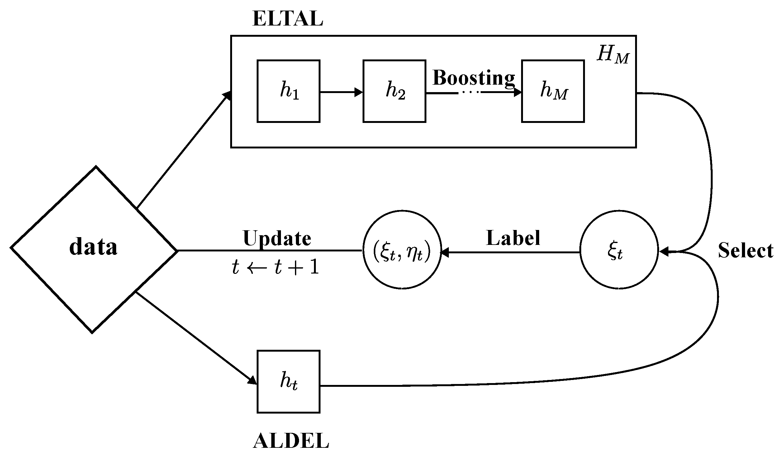
4.1. ELTAL in Boosting

To the best of our current knowledge, ActiveBoost was the first Boosting Algorithm to employ an active learning framework, as described by Wang et al. [37]. The authors were inspired by the stability of the naïve Bayes classifier when applied to the boosting process. Notably, the algorithm selects instances to be labeled after the boosting procedure, and therefore can be classified as an ELTAL approach. A disadvantage of this technique is that it necessitates the creation of numerous additional models without considering the underlying structure of the data.
This study presents a systematic and comprehensive approach to address the challenges of combining active learning with boosting. Our proposed algorithm, outlined in Algorithm 2, offers a more general solution to this problem. In recent years, a wide range of boosting procedures have been proposed, including Discrete AdaBoost, Real AdaBoost, Logit Boost, and Gentle AdaBoost, which all result in binary output hypotheses H = sign ( m = 1 M α m h m ) . To obtain a more detailed understanding of each candidate’s response towards H, we eliminate the sign ( · ) function, and intermediate weak learners’ results are required to be continuous to align with the proposed algorithm. As an example, consider the Real AdaBoost algorithm. At each iteration, the hypothesis is derived as h m ( x ) = 1 2 log { p m ( x ) / ( 1 p m ( x ) ) } , where p m ( x ) is the probability estimate that an instance x belongs to the positive class when the learner is trained on L t with W m . Weights of all hypotheses are identical in Real AdaBoost, while the weights of labeled instances are updated as w i , m w i , m exp { y i h m ( x i ) } before normalization.
Algorithm 2 Ensemble Learning on top of Active Learning (ELTAL) in Boosting
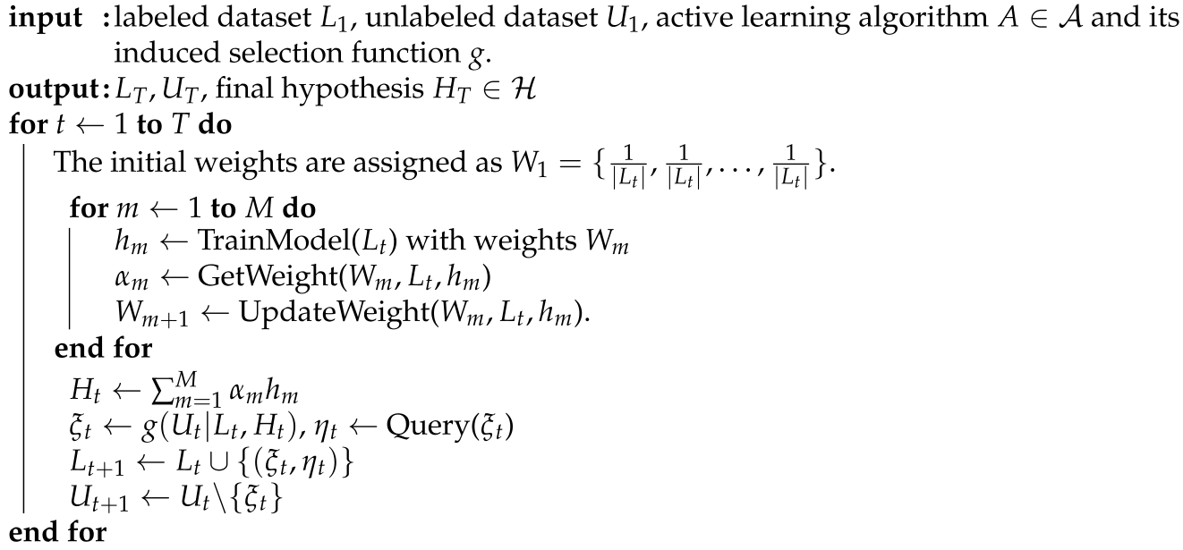
Stats 07 00008 i002
ELTAL algorithms select unlabeled instances when the ensembling procedure is complete. Although the information used for active learning is obtained from a strong learner, the computational burden is enormous since the ensembling procedure needs to be repeated after each update of the training set. ELTAL framework trains the model before implementing active learning. This non-overlapping structure of the framework is similar to the active learning approach used for basic machine learning models, thus provides a smooth transition from active learning for basic learners to ensembled learners. When the output of ensembled hypothesis is probabilistic, query strategies can be leveraged to identify the most informative samples. In this work, popular active learning approaches such as uncertainty sampling and expected error reduction are considered as selection criteria. To illustrate this, we provide some examples of the selection function g in ELTAL in Boosting.
  • Uncertainty Sampling [8]:
    g 1 ( U t | L t , H t ) = arg min x U t max { H t ( x ) , 1 H t ( x ) }
    g 2 ( U t | L t , H t ) = arg min x U t { H t ( x ) log H t ( x ) + ( 1 H t ( x ) ) log ( 1 H t ( x ) ) }
  • Expected Error Reduction [10]:
    g EER ( U t | L t , H t ) = arg min x U t { u { 1 , + 1 } Pr ( sign ( H t ( x ) ) = u | x , L t ) x i U t v { 1 , + 1 } Pr ( sign ( H t ( x i ) ) = v | x i , L t , x u ) log Pr ( sign ( H t ( x i ) ) = v | x i , L t , x u ) } ,
    where Pr ( sign ( H t ( x ) ) = u | x , L t ) is the probability that an instance x belongs to the class u when the hypothesis H t is trained on L t . The notation L t , x u = L t { ( x , u ) } is the extended labeled dataset when the instance is labeled as u and added to L t .

4.2. ALDEL in Boosting

For traditional AdaBoost-based algorithms, a new hypothesis is constructed at each iteration using all training data, with the weight function used to gauge the significance of each instance. If the i-th instance’s weight w i , m is close to zero, it has minimal impact on h m . Drawing motivation from this insight, we can initiate the boosting process by utilizing only a subset of the available training data. This subset can be treated as the labeled dataset within an active learning framework, with the remaining instances composing the unlabeled dataset. The incorporation of each instance into the subset can be determined based on whether its weight is zero. The indices of S n are rearranged to ensure that the first | L m | instances are labeled, and their weights are equally assigned as 1 / | L m | . This approach falls under the purview of ALDEL, which combines active learning and ensemble learning in a unified manner.
ALDEL in Boosting presents two significant challenges. Firstly, because the weight of the newly added instance has been zero until the last iteration, an approximate weight must be assigned to enable updates in subsequent iterations. Secondly, an appropriate selection criterion that aligns with the boosting objective must be chosen. Regardless of these two concerns, a general framework of ALDEL in Boosting is presented in Algorithm 3 and Figure 6 provides a visualization of Algorithm 3.
Algorithm 3 Active Learning During Ensemble Learning (ALDEL) in Boosting
Stats 07 00008 i003
The labeled instances are designated by the color green, while the unlabeled instances are colored red. In each iteration, the selected instance is colored blue, and the labeled instance utilized to match the weight is colored orange. After the completion of each iteration, the instances’ weights, orders, and colors are updated.
To fulfill the definition of “neighbor”, it’s essential to define a metric for measuring the distance between two instances. The underlying intuition is that if two instances yield similar exponential losses relative to the current hypothesis, they are probably of comparable importance to the boosting process. This similarity allows us to use the weight of one instance as a “proxy” or “fake” weight for the newly added instance. More precisely, we determine the distance between two instances based on the difference in their contributions to the exponential loss, as calculated with respect to the current hypothesis. This approach provides a practical means to assess the similarity between instances in the context of boosting, i.e.,
d ( x i , x j | h m ) = | exp ( y i h m ( x i ) ) exp ( y j h m ( x j ) ) |
In Real AdaBoost, it could also be rewritten as
d ( x i , x j | h m ) = | p m ( x i ) 1 p m ( x i ) y i 2 p m ( x j ) 1 p m ( x j ) y j 2 |
An instance’s importance is determined by its current weight, and the learning algorithm prioritizes instances that make the greatest contributions to the loss function. This notion sheds light on the following proposed AL querying strategy.
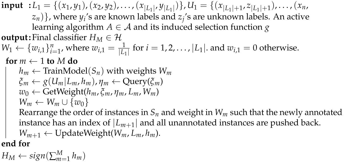
  • Expected Exponential Loss Maximization (EELM): The proposed querying strategy aims to select the instance that maximizes the expected exponential loss over all unlabeled data. Within the Real AdaBoost framework, the hypothesis h m ( x ) = 1 / 2 log p m ( x ) / ( 1 p m ( x ) ) is a transformation of the weighted probability estimates. The training and transformation steps of Real AdaBoost are identical to those of Discrete AdaBoost, with the objective of approximately optimizing J ( H ) in a stage-wise manner. The selection criterion could be described as    
    g ( U m | L m , h m ) = arg max x U m { p m ( x ) exp { h m ( x ) } + ( 1 p m ( x ) ) exp { h m ( x ) } } .
    It is important to note that the expected exponential loss in (9) can be expressed as a weighted conditional expectation E w on W m . For ease of presentation, we continue to denote p m as the weighted conditional probability. The selection criterion can also be viewed from an active learning perspective. By substituting the expression of p m ( x ) , the expected exponential loss reduces to 2 p m ( x ) ( 1 p m ( x ) ) , which is directly proportional to the standard deviation of p m ( x ) . Therefore, the selected instance has the highest variance among all instances in U m . This aligns with the principle of uncertainty sampling [8].

5. Active Learning in Stacking

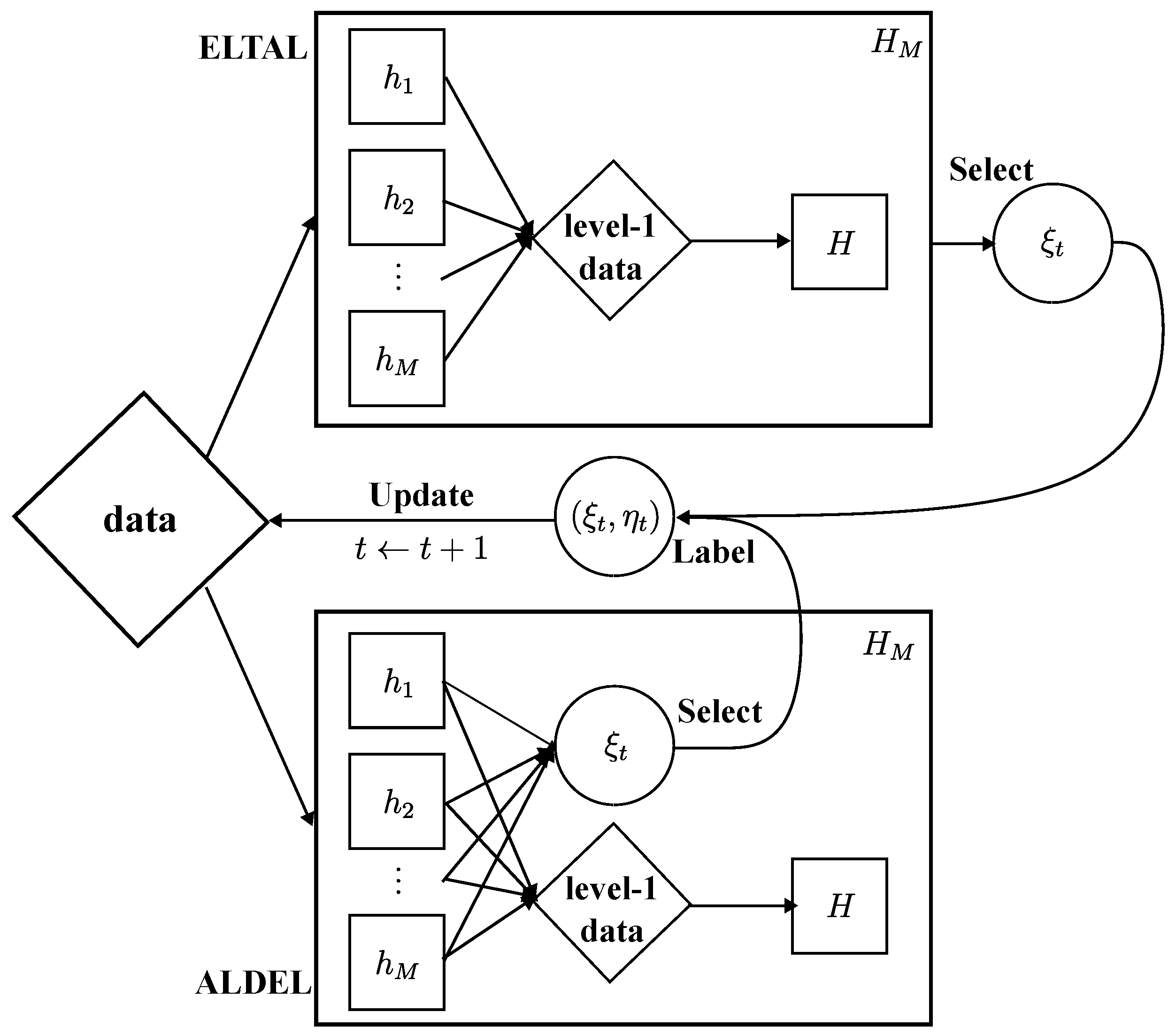
5.1. ELTAL in Stacking

ELTAL in Stacking is similar to ELTAL in Boosting in a way that the active learning is implemented after the ensembling procedure. Noticed that each lower-level learner is trained K times, one on each L t ( k ) . We define h t , m ( k ) as the m-th lower-level model that is trained on L t ( k ) . To get a probabilistic prediction for an instance in U t , we use the same averaging approach. More specifically, for an instance x j U t ,
z j m = h t , m ( x i ) , m = 1 , 2 , , M ,
where h t , m ( · ) = 1 K k = 1 K h t , m ( k ) ( · ) . If we denote L t as the collection { z j x j L t } and U t as the collection { z j x j U t } , the trained lower-level hypotheses create mappings from U t to U t and from L t to L t . In other words, L t is the concatenation of the cross-validated predictions on each fold and it is used for training the upper-level learner in the t-th iteration.
In this Algorithm, we assume that the selection function g 0 takes mapped sets L t and U t as arguments instead of L t and U t . Furthermore, we assume that the selection function g 0 ( U t ; θ t | L t , H t ) may depend on some extra tuning parameter θ t Θ . A general framework of ELTAL in Stacking is introduced in Algorithm 4.
Algorithm 4 Ensemble Learning on top of Active Learning (ELTAL) in Stacking
Stats 07 00008 i004
If we replace L t and U t by L t and U t , respectively, we could still use uncertainty sampling and expected error reduction as some examples for the choices of g such as (5)–(7).

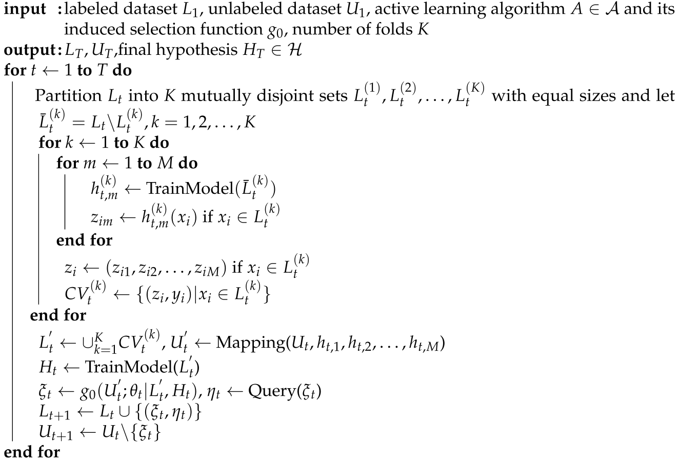
5.2. Two-Level Selection for ALDEL in Stacking

After the lower-level models are trained, ALDEL in Stacking can be applied to U t directly, or different lower-level models can individually select their preferred instances. However, this approach poses several challenges in deploying ALDEL with Stacking.
  • How to determine the appropriate selection criterion for each lower-level model. As the lower-level models are heterogeneous, it is reasonable to assume that their selection functions will differ.
  • How should the selected M instances be combined or integrated if each learner selects only one instance per iteration.
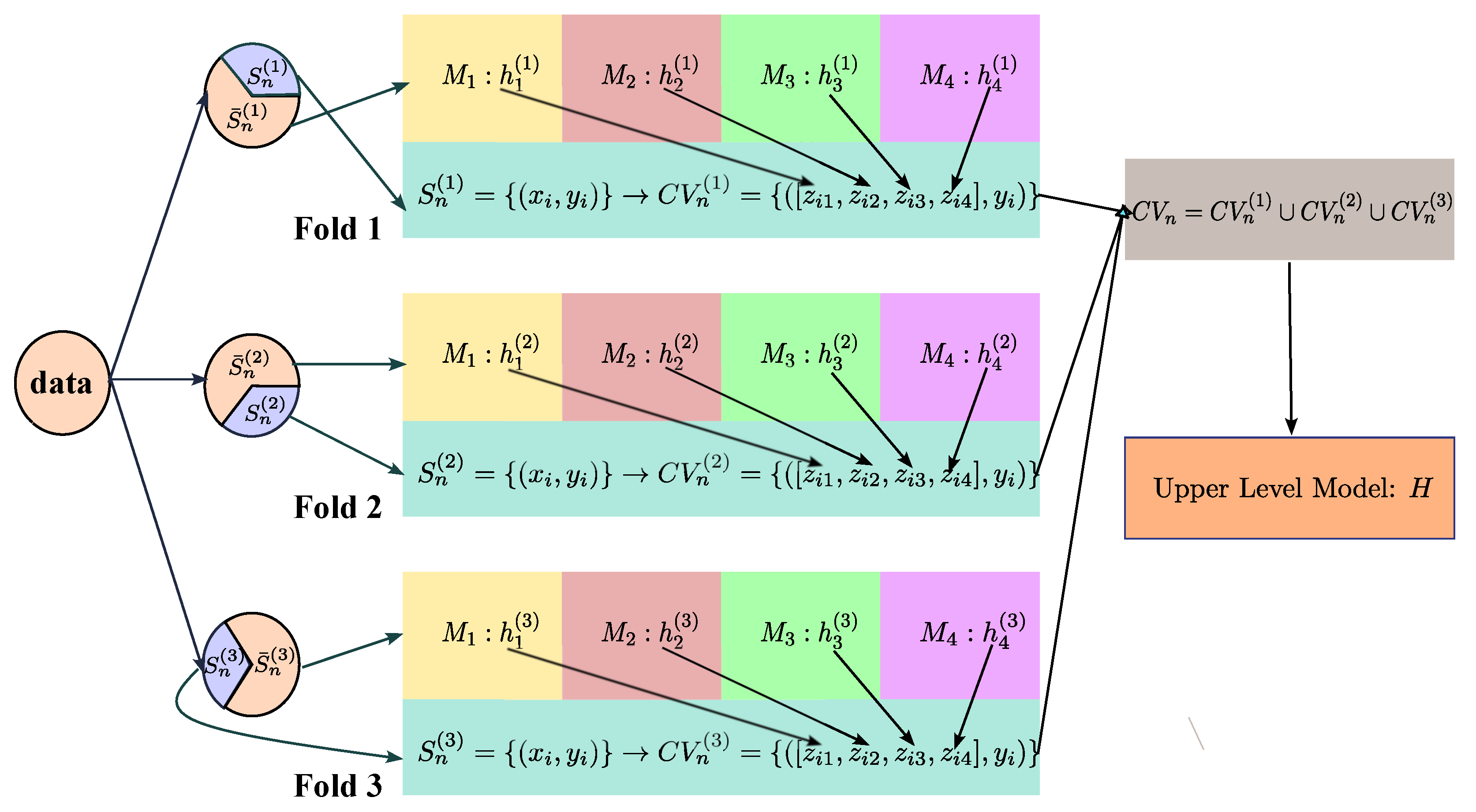
  • How to implement the active learning framework in the context of cross-validation.
Suppose the m-th lower-level model would apply the active learning algorithm A m A on the t-th iteration. The selection function g m G induced by A m takes some extra tuning parameters θ t , m Θ m . Similar to ELTAL in Stacking, each lower-level learner is trained on the cross-validation subset L ¯ t ( k ) and predicted on L t ( k ) on the t-th iteration.
The presented framework introduces a complication stemming from cross-validation. Specifically, each lower-level model is subjected to K iterations on distinct cross-validation subsets, but the selection function is intended to rely solely on a single replica. Consequently, it becomes necessary to construct a virtual hypothesis from the set of K hypotheses obtained from cross-validations. These hypotheses are homogeneous, and approximately ( k 2 ) | L t | / k instances are trained by every two learners simultaneously, which can be expressed mathematically as follows:
| L t ( i ) L t ( j ) | = ( K 2 ) | L t | K , i , j = 1 , 2 , , K
To integrate the results from all hypotheses, we utilize the decision function d ( x ) that was introduced in Section 2.2 for conventional parallel ensemble models. Thus, we treat the cross-validation results as parallel hypotheses that need to be ensembled, with h t , m ( k ) serving as the individual support of each hypothesis that an unlabeled instance belongs to the positive class. Given any x U t and the list of hypotheses h t , m ( 1 ) , h t , m ( 2 ) , , h t , m ( K ) , we define the “virtual” hypothesis h t , m as
h t , m ( · ) = d ( · | h t , m ( 1 ) ( · ) , , h t , m ( K ) ( · ) ) ,
where d ( · | ) denotes the decision function introduced in Section 2.2. The m-th lower-level model’s chosen instance is represented by ξ t , m , which is collected alongside the other selected instances as C t = { ξ t , 1 , ξ t , 2 , , ξ t , M } . When the goal is to introduce a single instance to the labeled dataset, an additional integration operation G must be conducted on C t . However, it is important to note that the labels of the instances in C t cannot be queried until the integration process is complete. It is not reasonable to retain only a single instance-label pair after integration when multiple instances have been labeled since this violates the general principle of active learning. To address this issue, we use the probabilistic output of each hypothesis to construct the integration function, which we refer to as the second-level selection. Algorithm 5 outlines a general framework of ALDEL in Stacking.
Next, we provide some intuition on the second-level selection in Algorithm 5. We select the instance from C t , such that it contribute most to improving the corresponding model. Notice that the selected instance will not be trained until the next iteration. At the ( t + 1 ) -th iteration, the m-th model is trained on L ¯ t + 1 ( k ) , a cross-validated set of L t + 1 and is measured on L t + 1 ( k ) . We define l m ( h m ( x ) , y ) : R × { 1 , + 1 } R + { 0 } as the loss function for the m-th lower-level model. A straightforward example for this loss function could be the cross-entropy loss as
l m ( h m ( x ) , y ) = [ y log h m ( x ) + ( 1 y ) log ( 1 h m ( x ) ) ]
We define ϕ m ( L t ) as the total loss when h t , m ( k ) is measured on L t ( k ) , i.e.,
ϕ m ( L t ) = k = 1 K x L t ( k ) l m ( h t , m ( k ) ( x ) , y )
After adding ξ t , m to the labeled dataset, the updated loss function under the worst case would be max { ϕ m ( L t { ( ξ t , m , 1 ) } ) , ϕ m ( L t { ( ξ t , m , 1 ) } ) } . We select the instance from C t such that ϕ m ( L t ) is increased minimally in the worst case. In other words,
G 1 ( C t ) = arg min ξ t , m C t max η t , m { 1 , + 1 } ϕ m ( L t { ( ξ t , m , η t , m ) } ) ϕ m ( L t ) ϕ m ( L t )
Similarly, we define l H ( H ( z ) , y ) : [ 0 , 1 ] × { 1 , + 1 } R + { 0 } as a loss function such as cross-entropy for the upper-level model. we denote ϕ H ( L t ) as the total upper-level loss when H t is measured on L t , i.e.,
ϕ H ( L t ) = x L t l H ( H t ( z ) , y )
The selection criterion would select the instance such that ϕ H ( L t + 1 ) is minimized, i.e.,
G 2 ( C t ) = arg min ξ t , m C t max η t , m { 1 , + 1 } ϕ H ( L t { ( ξ t , m , η t , m ) } )
Algorithm 5 Active Learning During Ensemble Learning (ALDEL) in Stacking
Stats 07 00008 i005

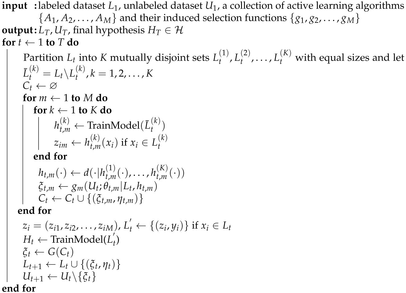
5.3. Direct Selection from the Lower-Level

In addition to the aforementioned two-level selection method, a viable alternative approach is to “take a step back” during the transition from basic to ensemble models in active learning. In other words, we employ the Query by Committee (QBC) technique for ALDEL method in Stacking. QBC is an active learning methodology where the selection is quantified by the degree of disagreement among a committee of pre-trained hypotheses [9,30]. In traditional QBC, the committee members are trained on a randomly selected subset of the labeled dataset, or even be combined with the bagging method [38,39] which employs resampling with replacement on L. The rationale behind this technique stemmed from the goal of inducing disagreement among the candidate hypotheses and thereby reducing the version space, which refers to the set of all hypotheses that perfectly predict all instances in the labeled dataset.
We leverage this idea to ALDEL in Stacking, where the available hypotheses come from M lower-level models. Since the committee of hypotheses in Stacking are outputted from different lower-level models trained on cross-validation datasets, resampling or subsampling procedures prior to traditional QBC are not necessary. The aim of QBC in Stacking should be querying an instance that induces maximal disagreement among all lower-level models. This motivation could alternatively be construed as emphasizing the indispensability of a upper-level model in cases where the degree of disagreement among committee members exceeds the capacity of a basic integration. When the instance is selected directly from the lower-level, the individual selection process in Algorithm 5 is discarded and replaced by a single selection ξ t = g QBC ( U t ; θ t | L t , h t , 1 , , h t , M )
The question to be determined now is the choice of the disagreement measurement. Settles [9] has suggested different choices of the disagreement measurement, including vote entropy, soft vote entropy, Kullback-Leibler (KL) divergence [40] and Jensen-Shannon divergence [41]. The choice of a disagreement metric should be customized to the specifics of the case at hand. Soft vote entropy is useful for measuring uncertainty across different classes, while KL divergence is more suited for assessing the degree of disagreement among committee members. Considering the diversity of models at the lower levels in stacking, KL divergence is the preferred method for identifying instances of disagreement at these levels, which can then be escalated for higher-level evaluation, i.e.,
g QBC ( U t ; θ t | L t , h t , 1 , h t , M ) = arg max x U t 1 M m = 1 M { h t , m ( x ) log h t , m ( x ) h ¯ t ( x ) + ( 1 h t , m ( x ) ) log 1 h t , m ( x ) 1 h ¯ t ( x ) } ,
where h ¯ t ( x ) = ( 1 / M ) m = 1 M h t , m ( x ) is the average decision from the committee.
So far, our attention has been directed towards informative-based querying strategies as classified in Kumar and Gupta [31]. These strategies are developed using information gleaned from a single instance relative to the current learning algorithm and do not take into account the structure inherent in the original data. Due to the selection functions used, the algorithms are often inclined to choose outliers, leading to extreme values in the selection function. To address this challenge, one could employ representative-based querying strategies, as classified in Kumar and Gupta [31], or in other words, exploration of feature correlation exploration techniques in Fu et al. [33].
The density-based approach is one of the most straightforward strategies that fall into this category. This approach entails the introduction of information density, which is defined as the product of an uncertainty measure and the average similarity between a candidate instance and all other unlabeled instances. It is reasonable to conceive lower-level models as a function that maps the set D X to [ 0 , 1 ] M . The columns in L t and U t , originating from lower-level models, effectively represent L t and U t respectively. Utilizing these predictions directly at the upper level makes density-based active learning (AL) on level-1 data a more practical and logical approach compared to using original data. Moreover, predictions from lower-level models often show high correlation for instances in the same fold. While cross-validation frameworks help in preventing overfitting in stacking models, exploring the feature structure of level-1 data remains a worthwhile pursuit. We propose the information density selection as follows
g ID ( U t ; β t | L t , h t , 1 , , h t , M ) = arg max x U t ϕ A ( z ) 1 | U t | z U t sim ( z , z ) β t ,
where ϕ A is an uncertainty measure on the upper-level such as the information entropy ( z log z + ( 1 z ) log ( 1 z ) ) and β t controls the importance tradeoff between the uncertainty and the density term at the t-th iteration. sim ( · , · ) is a similarity measure between a candidate instance and another instance in U t . To better capture the correlation between features in the level-1 data, we concentrate more on direction instead of magnitude when getting the similarity. Consequently, the cosine similarity
sim ( z , z ) = z z z z
is preferred.

6. Numerical Illustrations

6.1. Simulated Datasets

We perform a simulation to illustrate the numerical performances of the algorithms that are introduced in Section 4 and Section 5 in two-class classification tasks. Here the covariates come from a normal distribution, i.e., x i j N ( 0 , 1 ) , i = 1 , 2 , , n , j = 1 , 2 , , 5 , while the binary response vector is generated using the following model.
Pr ( y i = 1 ) = { 1 + exp ( p i 3 + 6 p i 2 9 p i + 2 ) } 1 / 3 , i = 1 , 2 , , n ,
where p i = w T x i and the true parameter is set as w = ( 1 , 1 , 1 , 1 , 1 , 1 ) T . We generate a set of S = 100 simulated datasets and each simulated dataset we generate has n = 5000 instances in total with a train test split of 70:30. In other words, for each of the 100 datasets, we use 3500 instances for training and 1500 for testing. The models with their corresponding active learning selection criteria and hyperparameters are summarized in Table 1. The weak learner to be boosted is chosen as the support vector machine (SVM) [42] with a Radial Basis Function (RBF) kernel that is defined as
K RBF ( x , x ) = exp ( γ | | x x | | 2 ) .
To incorporate active learning querying strategies into support vector machines (SVM) [42], we implement Platt scaling [43] to obtain a probabilistic output. This method involves training a logistic regression model with the distance of each sample from the decision boundary as the input and the true class labels as the output. The BOOST model is obtained by applying Real AdaBoost for 50 iterations to the SVM. Two distinct querying strategies are applied to both SVM and ELTAL in Boosting: UNIF and ENTROPY in (6). For ALDEL in Boosting, the EELM criterion in (9) is applied.
The STACK model employs four lower-level models, namely the support vector machine (SVM) with Radial Basis Function (RBF) kernel, Random Forest (RF) with 100 trees [44], Artificial Neural Networks with one hidden layer [45], and the Gradient Boosting Machine (GBM) [46]. To construct the mapping from L t to L t , we apply a 10-fold cross-validation, and obtain the “virtual” hypothesis from cross-validation as the average function. The upper-level model of the STACK model is logistic regression. In the Random Forest model, we can obtain a probabilistic output by using probability averaging. This method involves taking the average of the class probabilities predicted by each decision tree in the forest for a given input sample. Similar to ELTAL in Boosting, we apply UNIF and ENTROPY querying strategies to ELTAL in Stacking. As for ALDEL, we perform four active learning algorithms. For two-level selection, we employ Entropy in (6) as the first-level querying strategy, and G 1 in (11) and G 2 in (12) as the second-level selection criteria. Additionally, we employ Query by Committee approach in (13) to the lower-level models, utilizing KL divergence as the disagreement measure and a density-based method in (14) with entropy as the measure of uncertainty and cosine similarity as the measure of similarity. The value of the tuning parameter is set to a fixed value of β t = 1 .
In the simulation experiments, we randomly draw 50 instances from the training data, with 25 from each class, to form L 1 for each dataset. All models with an active learning component are initially trained using L 1 , and an instance is selected at each iteration until the stopping criterion is met. We partition the instances in L 1 equally into ten folds with five instances in each fold. This same partition is applied to all stacking-related models, including the STACK model. Specifically, the first selected instance is added to the first fold, and the subsequent instances are added sequentially to subsequent folds.
In terms of performance evaluation, we consider two metrics: Accuracy and Area Under the Receiver Operating Characteristic (ROC) Curve (AUC). The accuracy is defined as 1 err , where err is defined in Section 2. The ROC curve illustrates the trade-off between the true positive rate (TPR) and the false positive rate (FPR) at various threshold settings. The AUC is the area under the ROC curve and provides a single scalar value that summarizes the classifier’s overall performance across all possible threshold settings. At each iteration, the numerical performances of each model are evaluated on the test set.
In this simulation, we aim to demonstrate the numerical performances of active learning algorithms in the following aspects:
  • Comparison of applying the same active learning selection criterion to the weak learner, the boosted learner and the stacked learner. For instance, SVM-ENTROPY vs. ELTALB-ENTROPY vs. ELTALS-ENTROPY.
  • Comparison of different SVM-related and BOOST-related active learning algorithms with the vanilla SVM model, i.e., SVM-UNIF vs. SVM-ENTROPY vs. ELTALB-UNIF vs. ELTALB-ENTROPY vs. ALDEL-EELM.
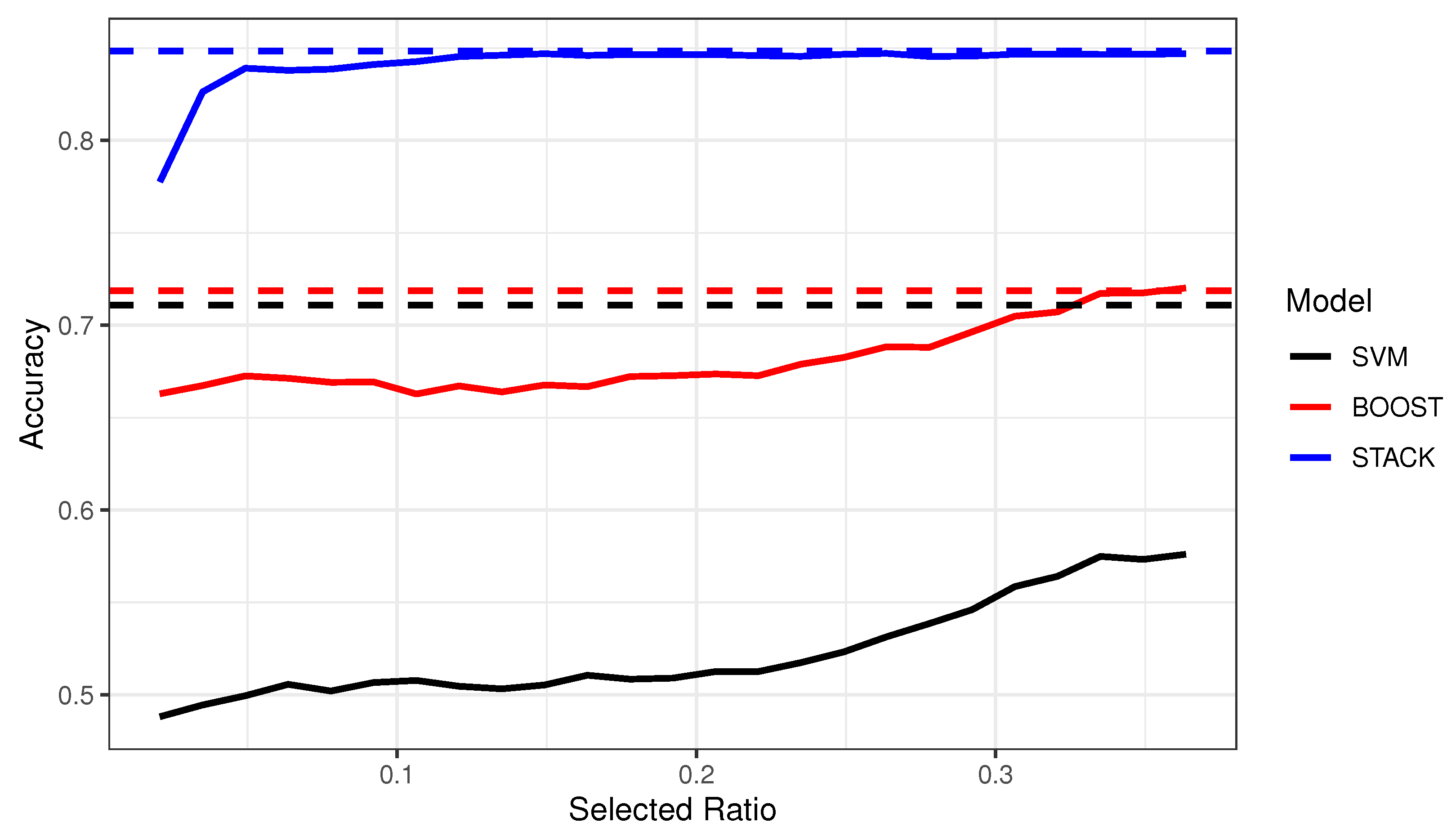
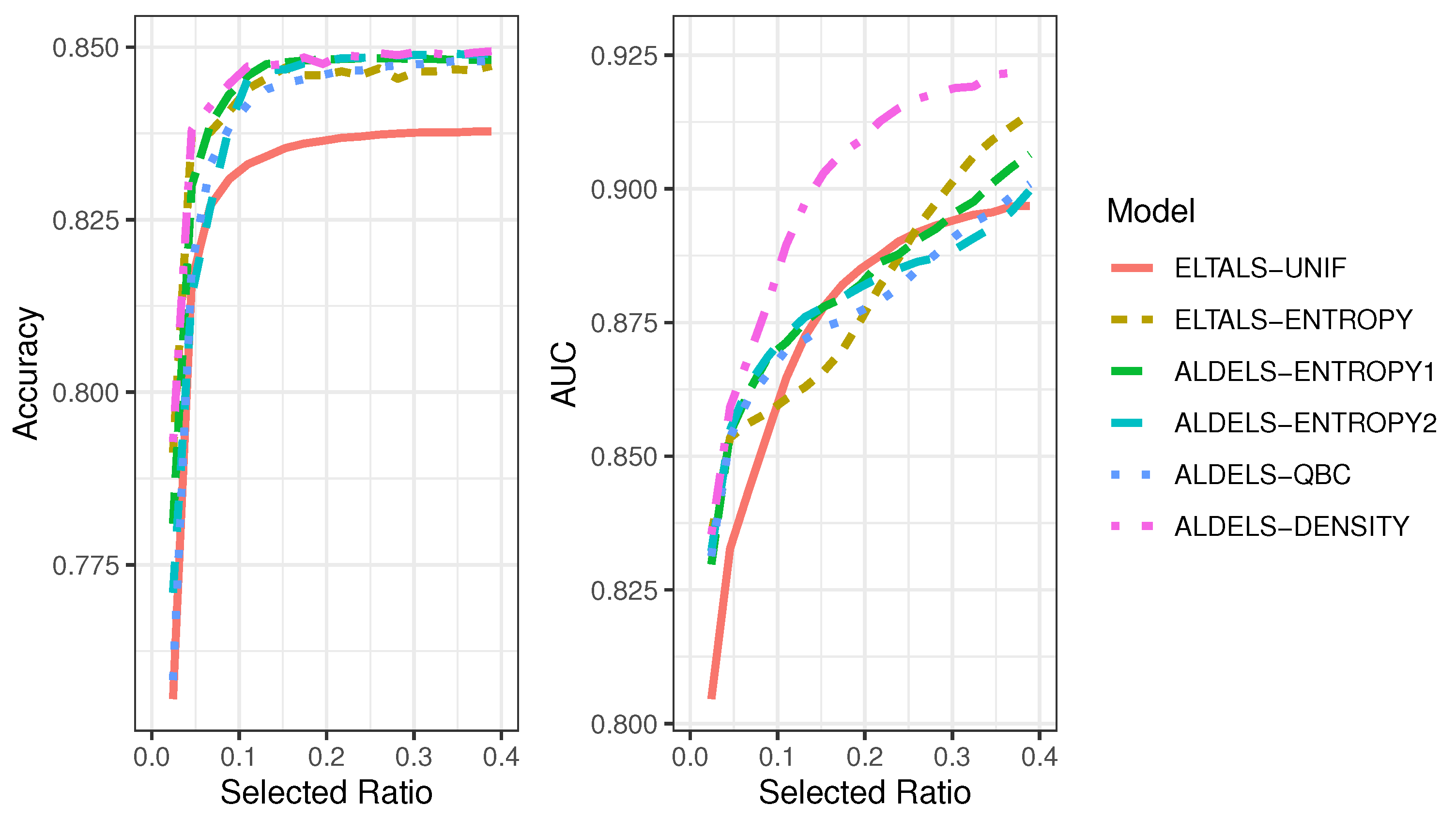
  • Comparison of different stacking-related active learning algorithms with the vanilla stacking model, i.e., STACK vs. ELTALS-UNIF vs. ELTALS-ENTROPY vs. ALDELS-ENTROPY1 vs. ALDEL-ENTROPY2 vs. ALDELS-QBC vs. ALDELS-DENSITY.
In Figure 7, the accuracy of SVM, BOOST, and STACK models trained on both the full dataset and labeled subsets selected by ENTROPY algorithms at different stages are displayed using dashed and solid lines, respectively. These accuracies were averaged across all S = 100 simulations. Concerning the full models, it is evident that both BOOST and STACK models display higher accuracies compared to SVM. Specifically, the accuracy of the STACK model surpasses SVM by an impressive 13%, whereas the BOOST model has a relatively marginal improvement of approximately 1%. As for active learning algorithms, the ranking of the three metric curves remains unaltered compared to those of the curves from full models. However, the accuracies of active learning algorithms are noticeably lower than those of the full models, and the differences between them become less significant as the algorithms select more instances.
Figure 8 presents the results of a comparative analysis of active learning algorithms applied to the SVM and the BOOST models, aimed at investigating the impact of boosting and active learning simultaneously. The figure provides insights into the efficacy of different active learning strategies, with the ENTROPY algorithm outperforming random sampling for both the SVM and the BOOST models, showcasing the potential of active learning. Furthermore, the ELTALB-UNIF and ELTALB-ENTROPY algorithms, applied to the BOOST model, exhibit superior performance compared to the SVM-UNIF and SVM-ENTROPY algorithms, highlighting the power of boosting. ALDELB-EELM, acting as a bridge between the SVM and BOOST models, demonstrates a performance level that falls between the BOOST-related and the SVM-related active learning algorithms when only a few instances are labeled and trained. These findings provide insights into the non-interfering improvement of SVM models from both active learning and Boosting. Boosting is effective for both models from the full and partial data selected by an active learning algorithm. On the other hand, an active learning algorithm can select more informative instances for labeling for both unboosted and boosted models.
Figure 9 illustrates the effectiveness of different active learning algorithms in the context of STACK. Their performances are assessed on test data using average accuracy and AUC metrics. The results show that ELTALS-UNIF significantly underperforms compared to other algorithms. In terms of AUC, ALDELS-DENSITY is more effective, surpassing the performance of both ALDEL and ELTAL algorithms. However, there is no marked performance difference among the other algorithms.
Table 2 presents a detailed summary of the outcomes obtained from the complete SVM, BOOST, and STACK models, in conjunction with the corresponding active learning techniques introduced in Table 1. The row for each full model delineates the time elapsed in seconds during training when 5%, 10%, 25% and 50% of all instances are used and the accuracy assessed on the test data using all available training data. Conversely, the row for each active learning algorithm describes the duration of selecting an unlabeled instance, as well as the improvement and deterioration in accuracy measured on the test data relative to the UNIF active learning algorithm and the full model at each stage of the selection process, respectively. The test data accuracy for the SVM model is reported as 71%, which is surpassed by the BOOST and STACK models, registering accuracies of 72% and 85%, respectively. When considering the training time, the SVM model exhibits a rapid training time of 0.04 s when trained on half of the available data. In comparison, the BOOST and STACK models require a longer training duration of 2.35 s and 4.29 s, respectively. The results from Table 2 demonstrate that the improvement in accuracy, as compared to SVM-UNIF, ELTALB-UNIF, and ELTALS-UNIF models, is consistently positive, indicating that the active learning algorithms employed are effective at all stages of selection.
At a selection ratio of 5%, ALDELB-EELM demonstrates a 13% accuracy improvement over SVM-UNIF, while experiencing a 16.5% reduction in accuracy relative to the full SVM model. It also has a significant improvement over SVM-ENTROPY up until the point where half of the instances are selected for use. The concurrent process of boosting and selection leads to a noteworthy reduction in the time required for instance selection (0.028 s compared to 0.669 s at a selection ratio of 5%). However, this approach also brings a reduction in accuracy of approximately 10% when 5% of instances are selected and about 17% when half of the instances are used.
Among the active learning algorithms associated with the STACK model, ALDELS-DENSITY exhibits a markedly longer selection time compared to its competitors. This is due to the computation of the similarity matrix for the unlabeled dataset at each iteration, as outlined in (14). The duration of this process becomes shorter when there are fewer unlabeled instances at a later stage. On the other hand, its performance is superior to other STACK-related AL algorithms. At a selection ratio of 5%, ALDELS-DENSITY incurs only a 3.5% additional error compared to the full STACK model, whereas other active learning algorithms show error increases ranging from 3.7% to 6.6%. The time taken to select data using ALDELS-ENTROPY1 and ALDELS-ENTROPY2 is longer compared to ELTALS-ENTROPY and ALDELS-QBC. This increased duration is because both ALDELS-ENTROPY1 and ALDELS-ENTROPY2 necessitate retraining of models, either at the lower or upper level, during their second-level selection process. ELTALS-ENTROPY boasts the shortest selection duration among all active learning algorithms linked to the STACK model. However, its selection process takes place only after the complete training of the STACK model, in contrast to other algorithms which require only the training of the lower-level models.
Table 2 demonstrates the mutual benefits of active learning and ensemble learning in enhancing a basic machine learning model. On one hand, active learning can significantly reduce the labeling and computational costs of an ensemble learning model. Despite using only a limited number of labeled instances, active learning can achieve efficiency comparable to that of the ensemble learning model that labels all instances. In other words, active learning addresses the primary computational weakness of ensemble learning models. On the other hand, ensemble learning can further improve the accuracy of a model generated by an active learning algorithm. While the core idea of active learning is to trade off some efficiency for lower labeling and computational costs, by combining with ensemble learning, active learning can create a model that requires labeling only a small number of instances but outperforms the basic model that labels all instances. For example, the SVM model in Table 2 has an accuracy of 71.1%. However, by labeling only 10% of the instances and with a negligible selection time of 0.64 s, ALDELS-QBC can build a stacking model with an accuracy of 78.2%.

6.2. Real Data Application

In this Section, we illustrate the performances of different active learning algorithms by two real data applications: fitness exercise pose classification and smoke detection.
The fitness exercise poses classification dataset includes physical poses from 500 Youtube video clips of people exercising. The fitness exercise dataset analyzed in this subsection is publicly available in the Kaggle repository, https://www.kaggle.com/datasets/muhannadtuameh/exercise-recognition, accessed on 27 February 2023. These videos are part of Countix, which is a real-world dataset that is focused on repeated actions. The covariates in the dataset are extracted from the MediaPipe framework which takes the video as an input and predicts the location of 33 pose landmarks such as left eye inner, left eye outer, left heel, etc. All instances come from 10 physical poses that can be further integrated into five different exercises. The accurate classification of the fitness exercises requires expertise in fitness training and thus we hope to apply active learning to mitigate the cost of manual labeling. We only keep the 296 cases from the jumping-jack and 231 from the pull-up classes for binary classification and there are 100 covariates in total.
The smoke detection dataset comprises numeric recordings of various indoor conditions and gas concentrations. Based on this, the detector decides whether it is alarming or not and is treated as the response variable. This dataset is publicly available in the Kaggle repository, https://www.kaggle.com/datasets/deepcontractor/smoke-detection-dataset, accessed on 28 February 2023. The original dataset has 60,000 observations and 13 covariates. Due to the imbalances between the two classes, 2500 instances are selected from each class to construct the dataset and all covariates are standardized.
For both real-world applications, 80% of instances are picked for training data, leaving the remaining to form the test data for measuring the classification models’ performances. The models are put to the test in S = 100 simulations of varying initializations, and all are trained on the same 50 instances, 25 from each class. We implement all models using the full dataset and all active learning algorithms introduced in Table 1 then feverishly query and label instances in sequence until the training dataset is depleted.
Table 3 and Table 4 show the average and standard error of Accuracy and F1-score metrics for all the active learning algorithms listed in Table 1 on the fitness exercise and smoke detection datasets, respectively. They illustrate how these algorithms perform with varying proportions of training data selected for labeling. The optimal non-stacking-related AL algorithm is highlighted in bold red, whereas the best stacking-related AL algorithm is represented in bold blue for each selection ratio.
In Table 3, the full SVM model achieves an accuracy of 80.2% on the test set, which is considerably lower than the boosted model’s accuracy of 96.23% and the stacking model’s accuracy of 94.08%. During the selection process, the SVM model with random selection performs better than the ENTROPY variant in uncertainty sampling. ELTALB-ENTROPY stands out by outperforming all other algorithms in terms of both accuracy and F1-score, which showcases the strength of active learning combined with boosting techniques. Although ALDELB-EELM does not surpass other boosting-related algorithms in terms of performance, it still exhibits superior accuracy and F1-score compared to the SVM-related active learning algorithms. As for stacking-related algorithms, all proposed active learning algorithms are superior to ELTALS-UNIF at all selection stages in terms of both accuracy and F1-score. Among these, ELTALS-ENTROPY becomes the winner among the rest, while ALDELS-DENSITY has a relative lower standard error but also a slightly lower averaged measurement. However, the selection of ALDELS-DENSITY does not depend on the training of upper-level, which is a plus for the algorithm compared to ELTALS-ENTROPY.
In Table 4, the full stacking model has a staggering 99.7% of accuracy and F1-score, which makes it more superior to the boosting model. With an approximate 90% of accuracy and F1-score, SVM still remains the worst full model. Here ELTALB-ENTROPY is still the best overall algorithm among all the SVM and boosting-related algorithms although the difference between ELTALB-UNIF and ELTALB-ENTROPY is no longer evident. For stacking-related algorithms, ALDELS-ENTROPY1, ALDELS-ENTROPY2 and ELTALS-ENTROPY all have a similar performance and those algorithms can create a stacking model that has 99.8% of accuracy when a merely 5% of instances are labeled and trained. The standard error of those three algorithms’ accuracy and F1-score remain as low as 0.01%, which makes them even more competitive.
Based on the analysis of real data applications, both the stacking and boosting approaches outperform the full SVM model. Throughout the selection stages, ELTALB-ENTROPY almost consistently proves to be the most competitive among all SVM and boosting-related models. Regarding stacking-related algorithms, each active learning algorithm demonstrates greater efficiency than the full SVM model, even when a small number of instances are selected. These findings motivate the adoption of active learning algorithms in ensemble learning models with a limited number of labeled instances instead of utilizing all the data and constructing a basic machine learning model. It is worth noting that while ALDELS-ENTROPY1 and ALDELS-ENTROPY2 employ different selection criteria based on loss at different levels, their performances are quite similar. Although it is challenging to pick a single preferred stacking-related active learning algorithm among the others, all of them exhibit significant improvements compared to random selection.

7. Discussion and Future Directions

This article presents a comprehensive framework for incorporating active learning into AdaBoost and stacking models. We introduce two distinct directions, namely ELTAL and ALDEL, which integrate active learning with ensemble learning based on the timing of instance selection. For each direction, we propose generalized algorithms applicable to both boosting and stacking.
In ELTAL algorithms, we provide examples using uncertainty sampling and random sampling to illustrate their application. In ALDEL for boosting, we introduce a query strategy that aims to select instances maximizing the expected exponential loss for labeling. The selected instance is then incorporated into the current labeled dataset for further boosting and training. In ALDEL for stacking, we present four active learning algorithms categorized as direct selection and two-level selection. The two-level selection allows individual lower-level models to independently select instances, followed by a second-level selection from the candidate instances. The direct selection treats lower-level training as a transformation of the input data and applies existing active learning algorithms to the probabilistic output of the lower-level models.
We evaluate all proposed algorithms against basic support vector machine model using simulated datasets and two real-world applications. The results demonstrate the significant performance enhancement achieved by ensemble learning, whether utilizing full data or partially labeled data from active learning algorithms. Moreover, we find that even a sub ensemble learning model trained on a small number of instances selected by an active learning algorithm can outperform a support vector machine trained on the entire dataset. The slight decrease in performance compared to the ensemble learning model trained on all instances is negligible.
There are certain limitations in this work that warrant further investigation. Firstly, the proposed active learning algorithms lack a solid theoretical foundation. While the success of AdaBoost is supported by the minimization of exponential loss and the conversion from weak learners to strong learners, the introduction of ALDEL for Boosting and the related query strategy are derived from intuition and demonstrated through numerical examples. Secondly, it is important to explore the optimization of ALDEL for Stacking. While the two-level selection allows each lower-level model to select their preferred instances independently, the independent selection process could be further enhanced by considering the most suitable query strategy for each model. This can draw insights from a wide range of active learning research conducted for different models. In our numerical illustrations, all lower-level selections are based on uncertainty sampling using cross-entropy. However, exploring different query strategies and determining their efficacy for specific real-world applications would be valuable. Currently, we have not provided sufficient intuition on when to utilize each query strategy or the rationale behind a query strategy being more competitive for a particular application.
To enhance our grasp and use of active learning algorithms within ensemble learning models, it’s crucial to overcome current limitations. Future research should concentrate on three key areas: providing theoretical foundations, optimizing active learning for Stacking methods, and determining the most effective query strategies for particular use cases. While we’ve laid out a basic framework for integrating active learning into ensemble learning, there’s a need for more detailed studies and advancements in optimization techniques in upcoming research.

Author Contributions

Conceptualization, Q.S.; methodology, Q.S.; software, Q.S.; validation, Q.S.; formal analysis, Q.S.; investigation, Q.S.; resources, Q.S.; data curation, Q.S.; writing—original draft preparation, Q.S.; writing—review and editing, S.K.G.; visualization, Q.S.; supervision, S.K.G.; project administration, Q.S. All authors have read and agreed to the published version of the manuscript.

Funding

This research received no external funding.

Institutional Review Board Statement

Not applicable.

Informed Consent Statement

This study utilized two publicly available datasets obtained from Kaggle, an online community of data scientists and machine learning practitioners. The datasets used are exercise recognition and smoke detection. Prior to their inclusion in this study, the datasets were reviewed for any ethical concerns. The datasets on Kaggle are provided under specific licenses that permit their free and open use for analytical and scientific research. The licenses associated with these datasets do not require individual consent as the data has been collected and processed in a manner consistent with Kaggle’s terms of service, which ensure that data providers have obtained all necessary consents and permissions for data collection and sharing.

Data Availability Statement

The data that were used in this article are publicly available in the Kaggle repository at https://www.kaggle.com/datasets/muhannadtuameh/exercise-recognition, accessed on 27 February 2023. and https://www.kaggle.com/datasets/deepcontractor/smoke-detection-dataset, accessed on 28 February 2023.

Conflicts of Interest

The authors declare that they have no competing interests.

References

  1. Sagi, O.; Rokach, L. Ensemble learning: A survey. Wiley Interdiscip. Rev. Data Min. Knowl. Discov. 2018, 8, e1249. [Google Scholar] [CrossRef]
  2. Freund, Y.; Schapire, R.E. Experiments with a new boosting algorithm. ICML 1996, 96, 148–156. [Google Scholar]
  3. Freund, Y.; Schapire, R.E. Game theory, on-line prediction and boosting. In Proceedings of the Ninth Annual Conference on Computational Learning Theory, Desenzano del Garda, Italy, 28 June–1 July 1996; pp. 325–332. [Google Scholar]
  4. Freund, Y.; Schapire, R.E. A decision-theoretic generalization of on-line learning and an application to boosting. J. Comput. Syst. Sci. 1997, 55, 119–139. [Google Scholar] [CrossRef]
  5. Friedman, J.H. Stochastic gradient boosting. Comput. Stat. Data Anal. 2002, 38, 367–378. [Google Scholar] [CrossRef]
  6. Wolpert, D.H. Stacked generalization. Neural Netw. 1992, 5, 241–259. [Google Scholar] [CrossRef]
  7. Breiman, L. Stacked regressions. Mach. Learn. 1996, 24, 49–64. [Google Scholar] [CrossRef]
  8. Lewis, D.D.; Gale, W.A. A sequential algorithm for training text classifiers. In Proceedings of the SIGIR’94, Dublin, Ireland, 3–6 July 1994; pp. 3–12. [Google Scholar]
  9. Settles, B. Active Learning Literature Survey; University of Wisconsin-Madison Department of Computer Sciences: Madison, WI, USA, 2009. [Google Scholar]
  10. Roy, N.; McCallum, A. Toward optimal active learning through sampling estimation of error reduction. Int. Conf. Mach. Learn. 2001, 441–448. [Google Scholar]
  11. Müller, B.; Reinhardt, J.; Strickland, M.T. Neural Networks: An Introduction; Springer Science & Business Media: Berlin/Heidelberg, Germany, 1995. [Google Scholar]
  12. Ren, P.; Xiao, Y.; Chang, X.; Huang, P.Y.; Li, Z.; Gupta, B.B.; Chen, X.; Wang, X. A survey of deep active learning. ACM Comput. Surv. (CSUR) 2021, 54, 1–40. [Google Scholar] [CrossRef]
  13. Abdar, M.; Pourpanah, F.; Hussain, S.; Rezazadegan, D.; Liu, L.; Ghavamzadeh, M.; Fieguth, P.; Cao, X.; Khosravi, A.; Acharya, U.R.; et al. A review of uncertainty quantification in deep learning: Techniques, applications and challenges. Inf. Fusion 2021, 76, 243–297. [Google Scholar] [CrossRef]
  14. Gal, Y.; Islam, R.; Ghahramani, Z. Deep bayesian active learning with image data. In Proceedings of the International Conference on Machine Learning, PMLR, Sydney, Australia, 6–11 August 2017; pp. 1183–1192. [Google Scholar]
  15. Beluch, W.H.; Genewein, T.; Nürnberger, A.; Köhler, J.M. The power of ensembles for active learning in image classification. In Proceedings of the IEEE Conference on Computer Vision and Pattern Recognition, Salt Lake City, UT, USA, 18–23 June 2018; pp. 9368–9377. [Google Scholar]
  16. Sener, O.; Savarese, S. A geometric approach to active learning for convolutional neural networks. arXiv 2017, arXiv:1708.00489. [Google Scholar]
  17. Pop, R.; Fulop, P. Deep ensemble bayesian active learning: Addressing the mode collapse issue in monte carlo dropout via ensembles. arXiv 2018, arXiv:1811.03897. [Google Scholar]
  18. Valiant, L.G. A theory of the learnable. Commun. ACM 1984, 27, 1134–1142. [Google Scholar] [CrossRef]
  19. Schapire, R.E. The strength of weak learnability. Mach. Learn. 1990, 5, 197–227. [Google Scholar] [CrossRef]
  20. Zhang, T.; Yu, B. Boosting with early stopping: Convergence and consistency. Ann. Stat. 2005, 1538. [Google Scholar] [CrossRef]
  21. Mease, D.; Wyner, A. Evidence Contrary to the Statistical View of Boosting. J. Mach. Learn. Res. 2008, 9, 131–156. [Google Scholar]
  22. Schapire, R.E.; Singer, Y. Improved boosting algorithms using confidence-rated predictions. In Proceedings of the Eleventh Annual Conference on Computational Learning Theory, Madison, WI, USA, 24–26 July 1998; pp. 80–91. [Google Scholar]
  23. Friedman, J.; Hastie, T.; Tibshirani, R. Additive logistic regression: A statistical view of boosting (with discussion and a rejoinder by the authors). Ann. Stat. 2000, 28, 337–407. [Google Scholar] [CrossRef]
  24. Polikar, R. Ensemble learning. In Ensemble Machine Learning: Methods and Applications; Springer: New York, NY, USA, 2012; pp. 1–34. [Google Scholar]
  25. Raftery, A.E.; Madigan, D.; Hoeting, J.A. Bayesian model averaging for linear regression models. J. Am. Stat. Assoc. 1997, 92, 179–191. [Google Scholar] [CrossRef]
  26. Hoeting, J.A.; Madigan, D.; Raftery, A.E.; Volinsky, C.T. Bayesian model averaging: A tutorial (with comments by M. Clyde, David Draper and EI George, and a rejoinder by the authors. Stat. Sci. 1999, 14, 382–417. [Google Scholar] [CrossRef]
  27. Wasserman, L. Bayesian model selection and model averaging. J. Math. Psychol. 2000, 44, 92–107. [Google Scholar] [CrossRef]
  28. Clarke, B. Comparing Bayes model averaging and stacking when model approximation error cannot be ignored. J. Mach. Learn. Res. 2003, 4, 683–712. [Google Scholar]
  29. Zhou, Z.H. Machine Learning; Springer Nature: Singapore, 2021. [Google Scholar]
  30. Seung, H.S.; Opper, M.; Sompolinsky, H. Query by committee. In Proceedings of the Fifth Annual Workshop on Computational Learning Theory, Pittsburgh, PA, USA, 27–29 July 1992; pp. 287–294. [Google Scholar]
  31. Kumar, P.; Gupta, A. Active learning query strategies for classification, regression, and clustering: A survey. J. Comput. Sci. Technol. 2020, 35, 913–945. [Google Scholar] [CrossRef]
  32. Settles, B.; Craven, M.; Ray, S. Multiple-instance active learning. Adv. Neural Inf. Process. Syst. 2007, 20, 1289–1296. [Google Scholar]
  33. Fu, Y.; Zhu, X.; Li, B. A survey on instance selection for active learning. Knowl. Inf. Syst. 2013, 35, 249–283. [Google Scholar] [CrossRef]
  34. Wu, Y.; Kozintsev, I.; Bouguet, J.Y.; Dulong, C. Sampling strategies for active learning in personal photo retrieval. In Proceedings of the 2006 IEEE International Conference on Multimedia and Expo, Toronto, ON, Canada, 9–12 July 2006; pp. 529–532. [Google Scholar]
  35. Li, X.; Guo, Y. Adaptive active learning for image classification. In Proceedings of the IEEE Conference on Computer Vision and Pattern Recognition, Portland, OR, USA, 23–28 June 2013; pp. 859–866. [Google Scholar]
  36. Yang, Y.; Loog, M. A variance maximization criterion for active learning. Pattern Recognit. 2018, 78, 358–370. [Google Scholar] [CrossRef]
  37. Wang, L.M.; Yuan, S.M.; Li, L.; Li, H.J. Boosting Naïve Bayes by active learning. In Proceedings of the 2004 International Conference on Machine Learning and Cybernetics (IEEE Cat. No. 04EX826), Shanghai, China, 26–29 August 2004; Volume 3, pp. 1383–1386. [Google Scholar]
  38. Abe, N. Query learning strategies using boosting and bagging. In Proceedings of the Fifteenth International Conference on Machine Learning, San Francisco, CA, USA, 24–27 July 1998; pp. 1–9. [Google Scholar]
  39. Breiman, L. Bagging predictors. Mach. Learn. 1996, 24, 123–140. [Google Scholar] [CrossRef]
  40. Kullback, S.; Leibler, R.A. On information and sufficiency. Ann. Math. Stat. 1951, 22, 79–86. [Google Scholar] [CrossRef]
  41. Menéndez, M.; Pardo, J.; Pardo, L.; Pardo, M. The jensen-shannon divergence. J. Frankl. Inst. 1997, 334, 307–318. [Google Scholar] [CrossRef]
  42. Hearst, M.A.; Dumais, S.T.; Osuna, E.; Platt, J.; Scholkopf, B. Support vector machines. IEEE Intell. Syst. Their Appl. 1998, 13, 18–28. [Google Scholar] [CrossRef]
  43. Platt, J. Probabilistic Outputs for Support Vector Machines and Comparisons to Regularized Likelihood Methods. Adv. Large Margin Classif. 2000, 10, 61–74. [Google Scholar]
  44. Breiman, L. Random forests. Mach. Learn. 2001, 45, 5–32. [Google Scholar] [CrossRef]
  45. Rumelhart, D.E.; Hinton, G.E.; Williams, R.J. Learning representations by back-propagating errors. Nature 1986, 323, 533–536. [Google Scholar] [CrossRef]
  46. Friedman, J.H. Greedy function approximation: A gradient boosting machine. Ann. Stat. 2001, 29, 1189–1232. [Google Scholar] [CrossRef]
Figure 1. An illustration of ensemble learning model.
Stats 07 00008 g001
Figure 2. A transition from classic active learning to ensemble active learning.
Stats 07 00008 g002
Figure 3. An illustration of cross-validated stacking model.
Stats 07 00008 g003
Figure 4. A visualization of ALDEL in Boosting and ELTAL in Boosting.
Stats 07 00008 g004
Figure 5. A visualization of ALDEL in Stacking and ELTAL in Stacking.
Stats 07 00008 g005
Figure 6. A visualization of ALDEL in Boosting.
Stats 07 00008 g006
Figure 7. A comparison of the average Accuracy for SVM, BOOST and STACK models trained on both full data and labeled subsets obtained through the ENTROPY active learning algorithms. The classification metrics are assessed on the test datasets at various stages of instance selection. Results for SVM, BOOST, and STACK are depicted with dashed lines, while solid lines represent the performances of the corresponding ENTROPY-variant models (i.e., SVM-ENTROPY, BOOST-ENTROPY, and ELTALB-ENTROPY, respectively).
Stats 07 00008 g007
Figure 8. A comparison of the average Accuracy and AUC for SVM models trained on the labeled subsets selected by various SVM-related or Boosting-related active learning algorithms. The classification metrics are assessed on the test datasets at various stages of instance selection.
Stats 07 00008 g008
Figure 9. A comparison of the average Accuracy and AUC for STACK models trained on the labeled subsets selected by various STACK-related active learning algorithms. The classification metrics are assessed on the test datasets at various stages of instance selection.
Stats 07 00008 g009
Table 1. A list of all models in the Simulation studies.
NameDescriptionActive Learning Selection CriterionHyperparameters
SVMSupport Vector Machine with
Radial Basis Function (RBF) kernel
N/Akernel parameter γ ,
regularization constant C
SVM-UNIFSame as SVMRandom selection
SVM-EntropySame as SVM Entropy variant in (6)
BOOSTReal AdaBoost Algorithm.
The basic learner is taken as SVM.
N/ABasic setup is the same as SVM;
SVM is boosted for
M = 50 times
ELTALB-UNIFELTAL in Boosting using Real AdaBoost
The basic learner is taken as SVM.
Random selection
ELTALB-EntropyELTAL in Boosting using Real AdaBoost
The basic learner is taken as SVM.
Entropy variant in (6)
ALDEL-EELMALDEL in Boosting using Real AdaBoost
The basic learner is taken as SVM.
EELM in (9)
STACKA Stacking Model. Lower-level models are
taken as SVM, Random Forest,
Artificial Neural Networks (ANN) and
Gradient Boosting Machine (GBM).
The upper-level
model is a logistic regression model.
N/ASVM: same as above

Random Forest:
number of trees: 100,
number of variables used
for splitting

ANN:
number of units, weight decay

GBM:
max depth, learning rate,
minimum number of
observations in each node,
number of trees: 100
ELTALS-UNIFELTAL in Stacking,
Models on both levels are the same as STACK.
Random selection
ELTALS-ENTROPYELTAL in Stacking,
Models on both levels are the same as STACK.
Entropy variant in uncertainty sampling
ALDELS-ENTROPY1ALDEL in Stacking,
Models on both levels are the same as STACK.
Lower-level selection is based on entropy
Upper-level selection is implemented using G 1
ALDELS-ENTROPY2ALDEL in Stacking,
Models on both levels are the same as STACK.
Lower-level selection is based on entropy
Upper-level selection is implemented using G 2
ALDELS-QBCALDEL in Stacking,
Models on both levels are the same as STACK.
Apply QBC to lower-level models.
KL divergence as the disagreement measure
ALDELS-DENSITYALDEL in Stacking,
Models on both levels are the same as STACK.
Apply Information Density AL on U t . Information
entropy is taken as ϕ A . Cosine similarity is used
Set β = 1
Table 2. Numerical Summaries of all SVM, BOOST and STACK-related active learning algorithms compared to the full model and the corresponding random sampling active learning algorithm in terms of average time elapsed during querying, training and the average improvement of Accuracy for the first 5%, 10%, 25%, 50% instances selected.
5%10%25%50%
Time vs. UNIF
vs. Full
Time vs. UNIF
vs. Full
Time vs. UNIF
vs. Full
Time vs. UNIF
vs. Full
SVM0.0060.7110.0070.7110.0160.7110.0400.711
SVM-
ENTROPY
0.0170.0710.0190.0320.0280.0090.0430.02
−0.218−0.211−0.204−0.180
ALDELB-
EELM
0.0280.1300.0310.0690.0470.0350.0840.031
−0.165−0.181−0.185−0.181
BOOST0.3320.7190.4200.7190.9240.7192.3490.719
ELTALB-
ENTROPY
0.6690.0320.8090.0341.3270.0292.0420.042
−0.052−0.049−0.048−0.020
STACK2.1620.8482.2200.8482.7970.8484.2870.848
ELTALS-
ENTROPY
0.5960.0300.6330.0190.7570.0140.8920.011
−0.037−0.021−0.009−0.005
ALDELS-
ENTROPY1
1.3750.0211.4510.0161.8770.0132.6890.012
−0.047−0.024−0.009−0.004
ALDELS-
ENTROPY2
1.7030.0081.8060.0052.2420.0093.2450.010
−0.059−0.035−0.013−0.006
ALDELS-
QBC
0.5990.0020.6440.0050.7490.0080.8780.009
−0.066−0.035−0.015−0.007
ALDELS-
DENSITY
44.160.03341.970.02239.010.01635.040.013
−0.035−0.018−0.007−0.003
Table 3. A summary of the mean and standard error of the accuracy and F1 score measured on the test set of the fitness exercise dataset when different sizes of instances are labeled and trained. Results from all full models and the sub models trained using the labeled subsets selected by different active learning algorithms are displayed. The accuracy and F-1 score are measured for S = 100 times with different initializations.
AccuracyF1 Score
Selected Ratio 20% 30% 50% 100% 20% 30% 50% 100%
SVM-UNIF79.64
(0.24)
80.17
(0.23)
79.61
(0.17)
80.2076.68
(0.43)
77.78
(0.45)
77.36
(0.29)
77.89
SVM-ENTROPY75.50
(1.46)
70.16
(2.22)
73.42
(1.01)
80.2072.82
(2.76)
60.26
(5.29)
73.00
(1.98)
77.89
ELTALB-UNIF85.16
(0.54)
87.33
(0.63)
87.91
(0.85)
96.2382.95
(1.45)
86.11
(1.61)
87.36
(2.00)
96.79
ELTALB-ENTROPY89.60
(0.62)
91.97
(1.01)
93.51
(0.61)
96.2387.60
(1.93)
91.64
(2.07)
93.75
(1.09)
96.79
ALDELB-EELM75.73
(1.72)
80.10
(1.61)
79.92
(1.66)
80.2077.58
(2.89)
81.60
(3.09)
62.80
(3.73)
77.89
ELTALS-UNIF80.45
(0.68)
83.49
(0.53)
85.86
(0.69)
94.0877.04
(1.14)
80.00
(1.31)
83.94
(1.12)
93.38
ELTALS-ENTROPY87.01
(0.68)
90.94
(0.70)
92.80
(0.50)
94.0887.35
(0.62)
90.13
(1.19)
92.51
(0.13)
93.38
ALDELS-ENTROPY182.05
(0.63)
87.62
(1.11)
91.31
(0.89)
94.0882.14
(2.11)
88.47
(1.23)
90.99
(1.17)
93.38
ALDELS-ENTROPY282.15
(1.27)
86.97
(1.34)
90.87
(0.90)
94.0884.73
(1.12)
87.08
(1.85)
90.19
(1.63)
93.38
ALDELS-QBC80.73
(1.00)
86.30
(0.62)
90.83
(0.42)
94.0878.96
(1.92)
84.11
(1.50)
89.54
(0.56)
93.38
ALDELS-DENSITY86.31
(0.33)
90.79
(0.23)
92.02
(0.28)
94.0885.04
(0.58)
89.90
(0.38)
91.73
(0.43)
93.38
Table 4. A summary of the mean and standard error of the accuracy and F1 score measured on the test set of the smoke detection dataset when different sizes of instances are labeled and trained. Results from all full models and the sub models trained using the labeled subsets selected by different active learning algorithms are displayed. The accuracy and F-1 are measured for S = 100 times with different initializations.
AccuracyF1 Score
Selected Ratio 5% 10% 25% 100% 5% 10% 25% 100%
SVM-UNIF88.66
(0.28)
88.94
(0.28)
89.64
(0.17)
89.7989.21
(0.27)
89.50
(0.29)
90.18
(0.19)
90.26
SVM-ENTROPY83.99
(3.05)
89.36
(1.21)
86.88
(1.52)
89.7983.41
(3.16)
89.42
(1.57)
85.80
(2.31)
90.26
ELTALB-UNIF89.03
(2.15)
91.23
(1.43)
92.87
(0.72)
95.0586.17
(3.63)
91.87
(2.04)
93.49
(0.50)
95.25
ELTALB-ENTROPY89.34
(2.95)
94.66
(1.98)
92.57
(2.32)
95.0585.43
(4.31)
94.45
(2.34)
90.87
(3.29)
95.25
ALDELB-EELM71.78
(3.47)
65.19
(2.92)
59.75
(2.85)
89.7963.61
(5.12)
65.47
(3.72)
62.85
(3.95)
90.26
ELTALS-UNIF98.60
(0.10)
99.05
(0.06)
99.53
(0.04)
99.7098.69
(0.10)
99.15
(0.05)
99.58
(0.03)
99.70
ELTALS-ENTROPY99.87
(0.01)
99.71
(0.01)
99.71
(0.01)
99.7099.86
(0.01)
99.71
(0.01)
99.71
(0.01)
99.70
ALDELS-ENTROPY199.85
(0.02)
99.77
(0.02)
99.69
(0.01)
99.7099.88
(0.01)
99.76
(0.01)
99.69
(0.01)
99.70
ALDELS-ENTROPY299.87
(0.01)
99.72
(0.01)
99.71
(0.01)
99.7099.87
(0.01)
99.73
(0.01)
99.71
(0.01)
99.70
ALDELS-QBC97.78
(0.26)
98.15
(0.17)
98.16
(0.22)
99.7099.73
(0.27)
98.13
(0.15)
98.15
(0.20)
99.70
ALDELS-DENSITY99.51
(0.23)
99.47
(0.18)
99.52
(0.13)
99.7099.53
(0.22)
99.48
(0.17)
99.53
(0.12)
99.70
Disclaimer/Publisher’s Note: The statements, opinions and data contained in all publications are solely those of the individual author(s) and contributor(s) and not of MDPI and/or the editor(s). MDPI and/or the editor(s) disclaim responsibility for any injury to people or property resulting from any ideas, methods, instructions or products referred to in the content.

