
Optimal Estimators of Cross-Partial Derivatives and Surrogates of Functions

1
Department DFR-ST, University of Guyane, 97346 Cayenne, France
2
228-UMR Espace-Dev, University of Guyane, University of Réunion, IRD, University of Montpellier, 34090 Montpellier, France
Stats 2024, 7(3), 697-718; https://doi.org/10.3390/stats7030042
Submission received: 31 May 2024
/
Revised: 4 July 2024
/
Accepted: 12 July 2024
/
Published: 14 July 2024
(This article belongs to the Section Statistical Methods)
Abstract
:Computing cross-partial derivatives using fewer model runs is relevant in modeling, such as stochastic approximation, derivative-based ANOVA, exploring complex models, and active subspaces. This paper introduces surrogates of all the cross-partial derivatives of functions by evaluating such functions at N randomized points and using a set of L constraints. Randomized points rely on independent, central, and symmetric variables. The associated estimators, based on model runs, reach the optimal rates of convergence (i.e., ), and the biases of our approximations do not suffer from the curse of dimensionality for a wide class of functions. Such results are used for (i) computing the main and upper bounds of sensitivity indices, and (ii) deriving emulators of simulators or surrogates of functions thanks to the derivative-based ANOVA. Simulations are presented to show the accuracy of our emulators and estimators of sensitivity indices. The plug-in estimates of indices using the U-statistics of one sample are numerically much stable.
Keywords:
derivative-based ANOVA; high-dimensional models; independent input variables; optimal estimators of derivatives; sensitivity analysisMSC:
62Fxx; 62J10; 49-XX; 26D101. Introduction
Derivatives are relevant in modeling, such as inverse problems, first-order and second-order stochastic approximation methods [1,2,3,4], exploring complex mathematical models or simulators, derivative-based ANOVA (Db-ANOVA) or exact expansions of functions, and active subspaces. First-order derivatives or gradients are sometime available in modeling. Instances are (i) models defined via their rates of change with respect to their inputs; (ii) implicit functions defined via their derivatives [5,6]; (iii) cases listed in [7,8] and the references therein.
In FANOVA and sensitivity analysis user and developer communities (see, e.g., [9,10,11,12,13,14]), screening of input variables and interactions of high-dimensional simulators is often performed before building emulators of such models using Gaussian processes [15,16,17,18,19], polynomial chaos expansions and SS-ANOVA [20,21], or other machine learning approaches. Emulators are fast-evaluated models that better approximate complex and/or too-expansive simulators. Efficient variance-based screening methods rely on the upper bounds of generalized sensitivity indices, including Sobol’ indices (see [14,22,23,24,25,26] for independent inputs and [27,28,29] for non-independent variables). Such upper bounds require the computations of cross-partial derivatives, even for simulators for which these computations are time-demanding or impossible. Also, active subspaces rely on the first-order derivatives for performing dimension reduction and then for approximating complex models [30,31,32,33].
For functions with full interactions, all the cross-partial derivatives are used in the integral representations of the infinitesimal increment of functions [34], and in the unanchored decompositions of functions in the Sobolev space [35]. Recently, such derivatives have become crucial in the Db-ANOVA representation of every smooth function, such as high-dimensional PDE models. Indeed, it is known, in [14], that every smooth function f admits an exact Db-ANOVA decomposition, that is, ,
where stands for the cross-partial derivative with respect to for any ; is a random vector of independent variables, supported on an open with margins s and densities s (i.e., ).
Computing all the cross-partial derivatives using a few model runs or evaluations of functions is challenging. Direct computations of accurate cross-partial derivatives were considered in [36,37] using the generalization of Richardson’s extrapolation. Such approximations of all the cross-partial derivatives require a number of model runs that strongly depends on the dimensionality (i.e., d). While adjoint-based methods can provide the gradients for some POE/PDE-based models using only one simulation of the adjoint models [38,39,40,41,42,43], note that computing the Hessian matrix requires running d second-order adjoint models in general, provided that such models are available (see [38,44]).
Stochastic perturbations methods or Monte Carlo approaches have been used in stochastic approximations (see, e.g., [1,2,3,4]), including derivative-free optimization (see [2,3,4,45,46,47,48] and the references therein), for computing the gradients and Hessian of functions. Such approaches lead to the estimates of gradients using a number of model runs that can be less than the dimensionality [48,49]. While gradients computations and the convergence analysis are considered in the first-order stochastic approximations, estimators of the Hessian matrices are investigated in the second-order stochastic approximations [2,50,51,52,53]. Most of such approaches rely on the Taylor expansions of functions and randomized kernels and/or a random vector that is uniformly distributed on the unit sphere. Nevertheless, independent variables are used in [48,50,53], and the approaches considered in [53,54] rely on the Stein identity [55]. Note that the upper bounds of the biases of such approximations depend on the dimensionality, except in the work [48] for the gradients only. Moreover, the convergence analysis for more than the second-order cross-partial derivatives are not available according to our knowledge.
Given a smooth function defined on , the motivation of this paper consists of proposing new approaches for deriving surrogates of cross-partial derivatives and derivative-based emulators of functions that
- Are simple to use and generic by making use of d independent variables that are symmetrically distributed about zero and a set of constraints;
- Lead to dimension-free upper bounds of the biases related to the approximations of cross-partial derivatives for a wide class of functions;
- Provide estimators of cross-partial derivatives that reach the optimal and parametric rates of convergence;
- Can be used for computing all the cross-partial derivatives and emulators of functions at given points using a small number of model runs.
In this paper, new expressions of cross-partial derivatives of any order are derived in Section 3 by combining the properties of (i) the generalized Richardson extrapolation approach so as to increase the approximations accuracy, and (ii) the Monte Carlo approaches based only on independent random variables that are symmetrically distributed about zero. Such expressions are followed by their order of approximations and biases. We also derive the estimators of such new expressions and their associated mean squared errors, including the rates of convergence for some classes of functions (see Section 3.3). Section 3.4 provides the derivative-based emulators of functions, depending on the strength of the interactions or (equivalently) the cross-partial derivatives, thanks to Equation (1). The strength of the interactions can be assessed using sensitivity analysis. Thus, Section 4 deals with the derivation of new expressions of sensitivity indices and their estimators by making use of the proposed surrogates of cross-partial derivatives. Simulations based on test functions are considered in Section 5 to show the accuracy of our approach, and we conclude this work in Section 6.
2. Preliminary
For an integer , let be a random vector of d independent and continuous variables with marginal cumulative distribution functions (CDFs) and probability density functions (PDFs) .
For a non-empty subset , we use for its cardinality (i.e., the number of elements in u) and . Also, we use for a subset of inputs, and we have the partition . Assume that:
Assumption 1
(A1). is a random vector of independent variables, supported on Ω.
Working with partial derivatives requires a specific mathematical space. Given an integer and an open set , consider a weak partial differentiable function [56,57] and a subset with . Namely, we use for the -th weak cross-partial derivatives of each component of f with respect to each with .
Likewise, given , denote and if and zero otherwise. Thus, taking yields . Moreover, denote , , and consider the Hölder space of -smooth functions given by
with , , and as weak cross-partial derivatives. We use for the Euclidean norm, for the -norm, for the expectation, and for the variance.
3. Surrogates of Cross-Partial Derivatives and New Emulators of Functions
3.1. New Expressions of Cross-Partial Derivatives
This section aims at providing expressions of cross-partial derivatives using the model of interest, and new independent random vectors. We provide approximated expressions of for all and the associated orders of approximations.
Given , consider with , , and denote with as d-dimensional random vectors of independent variables satisfying
Random vectors of d independent variables that are symmetrically distributed about zero are instances of , including the standard Gaussian random vector and symmetric uniform distributions about zero.
- Denote . The reals s are used for controlling the order of derivatives (i.e., ) we are interested in, while s help in selecting one particular derivative of order . Finally, s aim at defining a neighborhood of a sample point of that will be used. Thus, using and keeping in mind the variance of , we assume that
Assumption 2
(A2). .
Based on the above framework, Theorem 1 provides a new expression of the cross-partial derivatives of f. Recall that is the cardinality of u and .
Theorem 1.
Consider distinct s, and assume that with and (A2) holds. Then, for any with , there exists and coefficients such that
Proof.
The detailed proof is provided in Appendix A. □
In view of Theorem 1, we are able to compute all the cross-partial derivatives using the same evaluations of functions with the same or different order of approximations, depending on the constraints imposed to determine the coefficients (see Appendix A). While the setting or the constraints ; lead to the order , one can increase that order up to by using either or the full constraints given by . The last setting is going to improve the approximations and numerical computations of derivatives. Since increasing the number of constraints requires more evaluations of simulators, and in ANOVA-like decomposition of , it is common to neglect the higher-order components or, equivalently, the higher-order cross-partial derivatives thanks to Equation (1), the following parsimony number of constraints may be considered. Given an integer , controlling the partial derivatives of order up to can be performed using the constraints
Equation (3) gives approximations of all the cross-partial derivatives of where and if o is even and otherwise. This equation relies on the Vandermonde matrices and the generalized Vandermonde matrices, which ensure the existence and uniqueness of the coefficients for distinct values of s (i.e., ) because the determinant is of the form (see [58,59] for more details and the inverse of such matrices).
Remark 1.
When , we must have , . Thus, the coefficient does not necessarily depend on . Taking L for an even integer, the following nodes may be considered: . When L is odd, one may add 0 to the above set. Of course, other possibilities can be considered provided that .
Remark 2.
For a given , if we are only interested in all the cross-partial derivatives with , it is better to set in Equation (2).
Remark 3.
Links to other works.
Consider , and with . Using or or , our estimators of the first-order and the second-order cross-partial derivatives are very similar to the results obtained in [53].
Using the uniform perturbations and and , our estimators of the first-order and the second-order cross-partial derivatives are similar to those provided in [50]. However, we will see later that specific uniform distributions allow for obtaining dimension-free upper bounds of the biases.
3.2. Upper Bounds of Biases
To derive precise biases of our approximations provided in Theorem 1, different structural assumptions on the deterministic functions f and are considered. Assume that with is sufficient to define for any . Note that such an assumption does not depend on the dimensionality d. For the sequel of generality, we provide the upper bounds of the biases for any value of L by considering two sets of constraints.
Denote with a d-dimensional random vector of independent variables that are centered about zero and standardized (i.e., , ), and the set of such random vectors. For any , define
Corollary 1.
Consider distinct s and the constraints with . If and (A2) hold, then there is such that
Moreover, if with and , then
Proof.
See Appendix B for the detailed proof. □
In view of Corollary 1, one obtains the upper bounds that do not depend on the dimensionality d by choosing for instance. When , the choice is more appropriate. Corollary 1 provides the results for highly smooth functions. To be able to derive the optimal rates of convergence for a wide class of functions (i.e., ), Corollary 2 starts providing the biases for this class of functions under a specific set of constraints. To that end, define
Corollary 2.
For distinct s, consider and the constraints with . If and (A2) hold, then there is such that
Moreover, if with and , then
Proof.
See Appendix C. □
Note that the upper bounds derived in Corollary 2 depend on through and . Thus, taking and will give a dimension-free upper bound that does not increase with . The crucial role and importance of is highlighted in Section 3.3.
Remark 4.
Remark 5.
It is worth noting that we obtain exact approximations of in Corollary 1 for the class of functions described by
In general, exact approximations of are obtained when for highly smooth functions.
3.3. Convergence Analysis
Given a sample of , that is, and using Equation (2), the method of moments implies that the estimator of is given by
Statistically, it is common to measure the quality of an estimator using the mean squared error (MSE), including the rates of convergence. The MSEs can also help in determining the optimal value of . Theorem 2 provides such quantities under different assumptions. To that end, define
Theorem 2.
For distinct s, consider and with and . If and (A2) hold, then
Moreover, if with , then
Proof.
See Appendix D for the detailed proof. □
Theorem 2 provides the upper bounds of MSEs for the anisotropic case. Using a uniform bandwidth, that is, , reveals that such upper bounds clearly depend on the dimensionality of the function of interest. Indeed, we can check that the upper bounds of the MSEs provided in Equations (8) and (9) become, respectively,
By minimizing such upper bounds with respect to h, the optimal rates of convergence of the proposed estimators are derived in Corollary 3.
Corollary 3.
Under the assumptions made in Theorem 2, if , then
Proof.
See Appendix E for the detailed proof. □
The optimal rates of convergence obtained in Corollary 3 are far away from the parametric ones, and such rates decrease with . Nevertheless, such optimal rates are function of for any using . The maximum rate of convergence that can be reached is by taking .
To derive the optimal and parametric rates of convergence, let us now choose and with . Thus, we can see that the second terms of the upper bounds of the MSEs (provided in Theorem 2) are function of , but they are independent of h. This key observation leads to Corollary 4.
Corollary 4.
Under the assumptions made in Theorem 2, if ; and with , then we have
Proof.
The proof is straightforward since and if . □
It is worth noting that the upper bound of the squared bias obtained in Corollary 4 does not depend on the dimensionality thanks to . Also, the optimal and parametric rates of convergence are reached by means of model evaluations, and such model runs can still be used for computing for every with . Based on the same assumptions, it appears that the results provided in Corollary 4 are much more convenient for in higher dimensions, while those obtained in Corollary 3 are well suited for higher dimensions and for higher values of .
For highly smooth functions and for large values of and d, we are able to derive intermediate rates of convergence of the estimator of (see Theorem 3). To that end, consider an integer , , and denote with the largest integer that is less than b for any real b.
Theorem 3.
For an integer , consider . If and (A2) hold, then
Moreover, if with and , then
For a given , taking leads to
Proof.
Detailed proofs are provided in Appendix F. □
It turns out that the optimal rate of convergence derived in Theorem 3 is a trade-off between the sample size N and the dimensionality d. For instance, when , the optimal rate becomes , which improves the rate obtained in Corollary 3, but under different assumptions.
Remark 6.
Since the bias vanishes for the class of functions , taking yields (see Appendix G). Note that such an optimal rate of convergence is dimension-free.
3.4. Derivative-Based Emulators of Smooth Functions
Using Equation (1) and bearing in mind the estimators of the cross-derivatives provided in Section 3.3, this section aims at providing surrogates of smooth functions, also known as emulators. The general expression of the surrogate of f is given below.
Corollary 5.
For any , consider , . Assume that and (A1) and (A2) hold. Then, an approximation of f at is given by
The above plug-in estimator is consistent using the law of large numbers. For a given , it is worth noting that the choice of s is arbitrary, provided that such distributions are supported on an open neighborhood of .
Often, the higher-order cross-partial derivatives or, equivalently, the higher-order interactions among the model inputs almost vanish, leading us to consider the truncated expressions. Given an integer s with and keeping in mind the ANOVA decomposition, consider the class of functions that admit at most the s-th-order interactions, that is, . Truncating the functional expansion is a standard practice within the ANOVA-community, that is, is assumed in higher dimensions [10,12]. For such a class of functions, requiring with is sufficient to derive our results. Thus, the truncated surrogate of f is given by
Under the assumptions made in Corollary 5, reaches the optimal and parametric rate of convergence for the class of functions . For instance, taking leads to the first-order emulator of f, which relies only on the gradient information. Thus, provides accurate estimates of additive models of the form , where s are given functions. Likewise, allows for incorporating the second-order terms, but it requires the second-order cross-partial derivatives. Thus, it is relevant to find the class of functions which contains the model of interest before building emulators. The following section deals with such issues.
4. Applications: Computing Sensitivity Indices
In high-dimensional settings, reducing the dimension of functions is often achieved by using screening measures, that is, measures that can be used for quickly identifying non-relevant input variables. Screening measures based on the upper bounds of the total sensitivity indices rely on derivatives [14,23,24,25,60,61]. This section aims at providing optimal computations of upper bounds of the total indices, followed by the computations of the main indices using derivatives.
By evaluating the function f given by Equation (1) at a random vector using , one obtains a random vector of the model outputs. Generalized sensitivity indices, including Sobol’s indices, rely on the variance–covariance of sensitivity functionals (SFs), which are also random vectors containing the information about the overall contributions of inputs [14,26,62]. The derivative-based expressions of SFs are given below (see [14] for more details). Given , the interaction SF of the inputs is given by
and the first-order SF of is given by
Likewise, the total-interaction SF of is given by [14]
and the total SF of is given as [14]
For a single input , we have and . Among similarity measures [28,29], taking the variance–covariances of SFs, that is, , and , leads to [14]
Thus, is the upper bound of . Likewise, is the upper bound of (i.e., ), and it can be used for screening the input variables.
To provide new expressions of the screening measures and the main induces in the following proposition, denote with an i.i.d. copy of , and assume that
Assumption 3
(A3). has finite second-order moments.
Proposition 1.
Under the assumptions made in Corollary 4, assume that (A1)–(A3) hold. Then,
Proof.
The method of moments allows for deriving the estimators of and for all . For screening inputs of models, we provide the estimators of and for any . To that end, we are given four independent samples, that is, from , from , from , and from . Consistent estimators of and are, respectively, given by
The above (direct) estimators require model runs for obtaining the estimates for any . Additionally to such estimators, we derive the plug-in estimators, which are relevant in the presence of given data about the estimates of the first-order derivatives. To provide such estimators, we denote with a sample of known or estimates of the first-order derivatives (i.e., ). Using Equation (2), such estimates are obtained by considering or or and N. Keeping in mind Equations (12) and (13) and the U-statistic theory for one sample, the plug-in estimator of the main index of is given by
Likewise, the plug-in estimator of the upper bound of the total index of is given by
Note that the plug-in estimators are consistent and require a total of model runs for computing such indices, where is the number of model runs used for computing the gradient of f at .
5. Illustrations: Screening and Emulators of Models
5.1. Test Functions
5.1.1. Ishigami’s Function ()
The Ishigami function includes three independent inputs following a uniform distribution on , and it is given by
The sensitivity indices are , , , , , and .
5.1.2. Sobol’s g-Function ()
The g-function [63] includes ten independent inputs following a uniform distribution on , and it is defined as follows:
Note that such a function is differentiable almost everywhere. According to the values of , this function has different properties [23]:
- If , the values of sensitivity indices are , , , , and , . Thus, this function has a low effective dimension (function of type A), and it belongs to with (see Section 3.4).
- If , the first and total indices are given as follows: , . Thus, all inputs are important, but there is no interaction among these inputs. This function has a high effective dimension (function of type B). Note that it belongs to .
- If , the function belongs to the class of functions with important interactions among inputs. Indeed, we have and , . All the inputs are relevant due to important interactions (function of type C). Then, this function belongs to with .
5.2. Numerical Comparisons of Estimators
This section provides a comparison of the direct and plug-in estimators of the main indices and the upper bounds of the total indices using the test functions of Section 5.1. Different total budgets for the model evaluations are considered in this paper, that is, , 1000, 1500, 2000, 3000, 5000, 10,000, 15,000, 20,000. In the case of the plug-in estimators, we used . For generating different random values, Sobol’s sequence (scrambled = 3) from the R-package randtoolbox [64] is used. We replicated each estimation 30 times by randomly choosing the seed, and the reported results are the average of the 30 estimates.
Figure 1, Figure 2, Figure 3 and Figure 4 show the mean squared errors related to the estimates of the main indices for the Ishigami function, the g-functions of type A, type B, and type C, respectively. Each figure depicts the results for and . All the figures show the convergence and accuracy of our estimates using either or .
Likewise, Figure 5, Figure 6, Figure 7 and Figure 8 show the mean squared gaps (differences) between the true total index and its estimated upper bound for the Ishigami function, the g-functions of type A, type B, and type C, respectively.
It turns out that the plug-in estimators outperform the direct ones. Also, increasing the values of L gives the same results. Moreover, the direct estimators associated with fail to provide accuracy estimates (we do not report such results here). On the contrary, the plug-in estimates using are reported in Table 1 for the Ishigami function and in Table 2 for the three types of the g-function. Such results suggest considering or with for plug-in estimators when the total budget of model runs is small. For a larger budget of model runs, the direct estimators associated with and can be considered as well in practice.
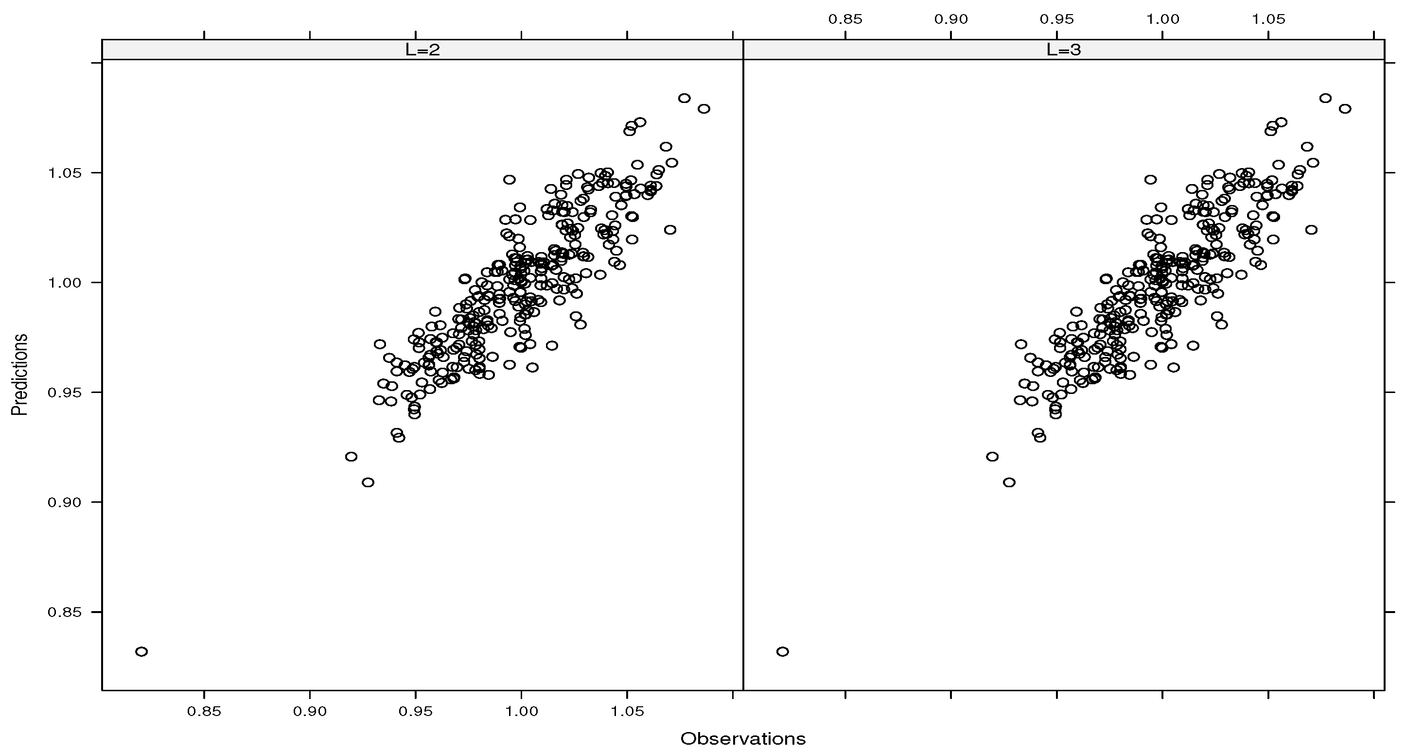
5.3. Emulations of the g-Function of Type B
Based on the results obtained in Section 5.2 (see Table 2), all the inputs are important in the case of the g-function of type B, meaning that the dimension reduction is not possible. Also, the estimated upper bounds suggest weak interactions among inputs. As expected, our estimated results confirm that the g-function of type B belongs to . Thus, an emulator of f based only on the first-order derivatives is sufficient. Using this information, we have derived the emulator of that function (i.e., ) under the assumptions made in Corollary 5 () and using with . For a given L, we used 300 model runs to build the emulator, and Figure 9 depicts the approximations of that function (called predictions) at the sample points involved in the construction of the emulator. Note that the evaluations of f at such sample points (called observations) are not directly used in the construction of such an emulator. It turns out from Figure 9 that provides predictions that are in line with the observations, showing the accuracy of our emulator.
6. Conclusions
In this paper, we firstly provided i) stochastic expressions of cross-partial derivatives of any order, followed by their biases, and ii) estimators of such expressions. Our estimators of the -th cross-partial derivatives () reach the parametric rates of convergence (i.e., ) by means of a set of constraints for the Hölder space of -smooth functions with . Moreover, we showed that the upper bounds of the biases of such estimators do not suffer from the curse of dimensionality. Secondly, the proposed surrogates of cross-partial derivatives are used for deriving (i) new derivative-based emulators of simulators or surrogates of models, even when a large number of model inputs contribute to the model outputs, and (ii) new repressions of the main sensitivity indices and the upper bounds of the total sensitivity indices.
Numerical simulations confirmed the accuracy of our approaches for not only screening the input variables, but also for identifying the class of functions that contains our simulator of interest, such as the class of functions with important or no interaction among inputs. This relevant information allows for designing and building the appropriate emulators of functions. In the case of the g-function of type B, our emulator of this function (based only on the first-order derivatives) provided approximations or predictions that are in line with the observations.
For functions with important interactions or, equivalently, for higher-order cross-partial derivatives, further numerical schemes are necessary to increase the numerical accuracy of the computations of such derivatives and predictions. Such perspectives will be investigated in the near future as well as the computations of the total sensitivity indices using the proposed surrogates of derivatives. Moreover, there is a need for a theoretical investigation to expect derivation of the parametric rates of convergence of the above estimators that do not suffer from the course of dimensionality. Working in rather than in may be helpful.
Funding
This research received no external funding.
Institutional Review Board Statement
Not applicable.
Informed Consent Statement
Not applicable.
Data Availability Statement
Data are contained within the article.
Acknowledgments
I would like to thank the three reviewers for their comments that helped improve my manuscript.
Conflicts of Interest
The author declares no conflict of interest.
Appendix A. Proof of Theorem 1
Firstly, as , denote and . The Taylor expansion of about of order is given by
Multiplying such an expansion by the constant , and taking the sum over , the expectation becomes
We can see that iff . Equation implies if and otherwise. Thus, using when is much more convenient, and it leads to , , which also implies that . We then obtain when or , and the fact that by independence. We can then write
using the change of variable . At this point, setting , and results in the approximation of of order .
Secondly, for , the constraints allow to eliminate some higher-order terms so as to reach the order . One can also use to increase the accuracy of approximations, but keeping the order when .
Appendix B. Proof of Corollary 1
- Let , , and consider the set . As , the expansion of giveswith the remainder term . Thus, and
Using , Theorem 1 implies that the absolute value of the bias is given by
as .
Using , the results hold because .
For with and , we have .
Appendix C. Proof of Corollary 2
- Let . As , we can writewith the remainder term . Using and Theorem 1, the results hold by analogy to the proof of Corollary 1. Indeed, if , then
For with and , we have
Appendix D. Proof of Theorem 2
As implies that with , we have
Using the fact that for , we can write
which leads to .
By taking the variance of the proposed estimator, we have
where .
If , .
The results hold using Corollary 2 and the fact that .
Appendix E. Proof of Corollary 3
Let , and . By minimizing , we obtain
and
Appendix F. Proof of Theorem 3
The first two results hold by combining the biases obtained in Corollary 1 and the upper bounds of the variance provided in Theorem 2.
For the last result, let , and . By minimizing the last upper bound, we obtain and
Appendix G. On Remark 6
The variance is and
References
- Robbins, H.; Monro, S. A Stochastic Approximation Method. Ann. Math. Stat. 1951, 22, 400–407. [Google Scholar] [CrossRef]
- Fabian, V. Stochastic approximation. In Optimizing Methods in Statistics; Elsevier: Amsterdam, The Netherlands, 1971; pp. 439–470. [Google Scholar]
- Nemirovsky, A.; Yudin, D. Problem Complexity and Method Efficiency in Optimization; Wiley & Sons: New York, NY, USA, 1983. [Google Scholar]
- Polyak, B.; Tsybakov, A. Optimal accuracy orders of stochastic approximation algorithms. Probl. Peredachi Inf. 1990, 2, 45–53. [Google Scholar]
- Cristea, M. On global implicit function theorem. J. Math. Anal. Appl. 2017, 456, 1290–1302. [Google Scholar] [CrossRef]
- Lamboni, M. Derivative formulas and gradient of functions with non-independent variables. Axioms 2023, 12, 845. [Google Scholar] [CrossRef]
- Morris, M.D.; Mitchell, T.J.; Ylvisaker, D. Bayesian design and analysis of computer experiments: Use of derivatives in surface prediction. Technometrics 1993, 35, 243–255. [Google Scholar] [CrossRef]
- Solak, E.; Murray-Smith, R.; Leithead, W.; Leith, D.; Rasmussen, C. Derivative observations in Gaussian process models of dynamic systems. In Advances in Neural Information Processing Systems 15; MIT Press: Cambridge, MA, USA, 2002. [Google Scholar]
- Hoeffding, W. A class of statistics with asymptotically normal distribution. Ann. Math. Stat. 1948, 19, 293–325. [Google Scholar] [CrossRef]
- Efron, B.; Stein, C. The jacknife estimate of variance. Ann. Stat. 1981, 9, 586–596. [Google Scholar] [CrossRef]
- Sobol, I.M. Sensitivity analysis for non-linear mathematical models. Math. Model. Comput. Exp. 1993, 1, 407–414. [Google Scholar]
- Rabitz, H. General foundations of high dimensional model representations. J. Math. Chem. 1999, 25, 197–233. [Google Scholar] [CrossRef]
- Saltelli, A.; Chan, K.; Scott, E. Variance-Based Methods, Probability and Statistics; John Wiley and Sons: Hoboken, NJ, USA, 2000. [Google Scholar]
- Lamboni, M. Weak derivative-based expansion of functions: ANOVA and some inequalities. Math. Comput. Simul. 2022, 194, 691–718. [Google Scholar] [CrossRef]
- Currin, C.; Mitchell, T.; Morris, M.; Ylvisaker, D. Bayesian prediction of deterministic functions, with applications to the design and analysis of computer experiments. J. Am. Stat. Assoc. 1991, 86, 953–963. [Google Scholar] [CrossRef]
- Oakley, J.E.; O’Hagan, A. Probabilistic sensitivity analysis of complex models: A bayesian approach. J. R. Stat. Soc. Ser. B Stat. Methodol. 2004, 66, 751–769. [Google Scholar] [CrossRef]
- Conti, S.; O’Hagan, A. Bayesian emulation of complex multi-output and dynamic computer models. J. Stat. Plan. Inference 2010, 140, 640–651. [Google Scholar] [CrossRef]
- Haylock, R.G.; O’Hagan, A.; Bernardo, J.M. On inference for outputs of computationally expensive algorithms with uncertainty on the inputs. In Bayesian Statistics 5: Proceedings of the Fifth Valencia International Meeting; Oxford Academic: Oxford, UK, 1996; Volume 5, pp. 629–638. [Google Scholar]
- Kennedy, M.C.; O’Hagan, A. Bayesian calibration of computer models. J. R. Stat. Soc. Ser. B Stat. Methodol. 2001, 63, 425–464. [Google Scholar] [CrossRef]
- Sudret, B. Global sensitivity analysis using polynomial chaos expansions. Reliab. Eng. Syst. Saf. 2008, 93, 964–979. [Google Scholar] [CrossRef]
- Wahba, G. An introduction to (smoothing spline) anova models in rkhs with examples in geographical data, medicine, atmospheric science and machine learning. arXiv 2004, arXiv:math/0410419. [Google Scholar] [CrossRef]
- Sobol, I.M.; Kucherenko, S. Derivative based global sensitivity measures and the link with global sensitivity indices. Math. Comput. Simul. 2009, 79, 3009–3017. [Google Scholar] [CrossRef]
- Kucherenko, S.; Rodriguez-Fernandez, M.; Pantelides, C.; Shah, N. Monte Carlo evaluation of derivative-based global sensitivity measures. Reliab. Eng. Syst. Saf. 2009, 94, 1135–1148. [Google Scholar] [CrossRef]
- Lamboni, M.; Iooss, B.; Popelin, A.-L.; Gamboa, F. Derivative-based global sensitivity measures: General links with Sobol’ indices and numerical tests. Math. Comput. Simul. 2013, 87, 45–54. [Google Scholar] [CrossRef]
- Roustant, O.; Fruth, J.; Iooss, B.; Kuhnt, S. Crossed-derivative based sensitivity measures for interaction screening. Math. Comput. Simul. 2014, 105, 105–118. [Google Scholar] [CrossRef]
- Lamboni, M. Derivative-based generalized sensitivity indices and Sobol’ indices. Math. Comput. Simul. 2020, 170, 236–256. [Google Scholar] [CrossRef]
- Lamboni, M.; Kucherenko, S. Multivariate sensitivity analysis and derivative-based global sensitivity measures with dependent variables. Reliab. Eng. Syst. Saf. 2021, 212, 107519. [Google Scholar] [CrossRef]
- Lamboni, M. Measuring inputs-outputs association for time-dependent hazard models under safety objectives using kernels. Int. J. Uncertain. Quantif. 2024, 1–17. [Google Scholar] [CrossRef]
- Lamboni, M. Kernel-based measures of association between inputs and outputs using ANOVA. Sankhya A 2024. [CrossRef]
- Russi, T.M. Uncertainty Quantification with Experimental Data and Complex System Models; Spring: Berlin/Heidelberg, Germany, 2010. [Google Scholar]
- Constantine, P.; Dow, E.; Wang, S. Active subspace methods in theory and practice: Applications to kriging surfaces. SIAM J. Sci. Comput. 2014, 36, 1500–1524. [Google Scholar] [CrossRef]
- Zahm, O.; Constantine, P.G.; Prieur, C.; Marzouk, Y.M. Gradient-based dimension reduction of multivariate vector-valued functions. SIAM J. Sci. Comput. 2020, 42, A534–A558. [Google Scholar] [CrossRef]
- Kucherenko, S.; Shah, N.; Zaccheus, O. Application of Active Subspaces for Model Reduction and Identification of Design Space; Springer: Berlin/Heidelberg, Germany, 2024; pp. 412–418. [Google Scholar]
- Kubicek, M.; Minisci, E.; Cisternino, M. High dimensional sensitivity analysis using surrogate modeling and high dimensional model representation. Int. J. Uncertain. Quantif. 2015, 5, 393–414. [Google Scholar] [CrossRef]
- Kuo, F.; Sloan, I.; Wasilkowski, G.; Woźniakowski, H. On decompositions of multivariate functions. Math. Comput. 2010, 79, 953–966. [Google Scholar] [CrossRef]
- Bates, D.; Watts, D. Relative curvature measures of nonlinearity. J. Royal Stat. Soc. Ser. B 1980, 42, 1–25. [Google Scholar] [CrossRef]
- Guidotti, E. calculus: High-dimensional numerical and symbolic calculus in R. J. Stat. Softw. 2022, 104, 1–37. [Google Scholar] [CrossRef]
- Le Dimet, F.-X.; Talagrand, O. Variational algorithms for analysis and assimilation of meteorological observations: Theoretical aspects. Tellus A Dyn. Meteorol. Oceanogr. 1986, 38, 97–110. [Google Scholar] [CrossRef]
- Le Dimet, F.X.; Ngodock, H.E.; Luong, B.; Verron, J. Sensitivity analysis in variational data assimilation. J. Meteorol. Soc. Jpn. 1997, 75, 245–255. [Google Scholar] [CrossRef]
- Cacuci, D.G. Sensitivity and Uncertainty Analysis—Theory, Chapman & Hall; CRC: Boca Raton, FL, USA, 2005. [Google Scholar]
- Gunzburger, M.D. Perspectives in Flow Control and Optimization; SIAM: Philadelphia, PA, USA, 2003. [Google Scholar]
- Borzi, A.; Schulz, V. Computational Optimization of Systems Governed by Partial Differential Equations; SIAM: Philadelphia, PA, USA, 2012. [Google Scholar]
- Ghanem, R.; Higdon, D.; Owhadi, H. Handbook of Uncertainty Quantification; Springer International Publishing: Berlin/Heidelberg, Germany, 2017. [Google Scholar]
- Wang, Z.; Navon, I.M.; Le Dimet, F.-X.; Zou, X. The second order adjoint analysis: Theory and applications. Meteorol. Atmos. Phys. 1992, 50, 3–20. [Google Scholar] [CrossRef]
- Agarwal, A.; Dekel, O.; Xiao, L. Optimal algorithms for online convex optimization with multi-point bandit feedback. In Proceedings of the 23rd Conference on Learning Theory, Haifa, Israel, 27–29 June 2010; pp. 28–40. [Google Scholar]
- Bach, F.; Perchet, V. Highly-smooth zero-th order online optimization. In Proceedings of the 29th Annual Conference on Learning Theory, New York, NY, USA, 23–26 June 2016; Feldman, V., Rakhlin, A., Shamir, O., Eds.; Volume 49, pp. 257–283. [Google Scholar]
- Akhavan, A.; Pontil, M.; Tsybakov, A.B. Exploiting Higher Order Smoothness in Derivative-Free Optimization and Continuous Bandits, NIPS’20; Curran Associates Inc.: Red Hook, NY, USA, 2020. [Google Scholar]
- Lamboni, M. Optimal and efficient approximations of gradients of functions with nonindependent variables. Axioms 2024, 13, 426. [Google Scholar] [CrossRef]
- Patelli, E.; Pradlwarter, H. Monte Carlo gradient estimation in high dimensions. Int. J. Numer. Methods Eng. 2010, 81, 172–188. [Google Scholar] [CrossRef]
- Prashanth, L.; Bhatnagar, S.; Fu, M.; Marcus, S. Adaptive system optimization using random directions stochastic approximation. IEEE Trans. Autom. Control. 2016, 62, 2223–2238. [Google Scholar]
- Agarwal, N.; Bullins, B.; Hazan, E. Second-order stochastic optimization for machine learning in linear time. J. Mach. Learn. Res. 2017, 18, 4148–4187. [Google Scholar]
- Zhu, J.; Wang, L.; Spall, J.C. Efficient implementation of second-order stochastic approximation algorithms in high-dimensional problems. IEEE Trans. Neural Netw. Learn. Syst. 2020, 31, 3087–3099. [Google Scholar] [CrossRef] [PubMed]
- Zhu, J. Hessian estimation via stein’s identity in black-box problems. In Proceedings of the 2nd Mathematical and Scientific Machine Learning Conference, Online, 15–17 August 2022; Bruna, J., Hesthaven, J., Zdeborova, L., Eds.; Volume 145 of Proceedings of Machine Learning Research, PMLR. pp. 1161–1178. [Google Scholar]
- Erdogdu, M.A. Newton-stein method: A second order method for glms via stein’ s lemma. In Advances in Neural Information Processing Systems; Cortes, C., Lawrence, N., Lee, D., Sugiyama, M., Garnett, R., Eds.; Curran Associates, Inc.: Red Hook, NY, USA, 2015; Volume 28. [Google Scholar]
- Stein, C.; Diaconis, P.; Holmes, S.; Reinert, G. Use of exchangeable pairs in the analysis of simulations. Lect.-Notes-Monogr. Ser. 2004, 46, 1–26. [Google Scholar]
- Zemanian, A. Distribution Theory and Transform Analysis: An Introduction to Generalized Functions, with Applications, Dover Books on Advanced Mathematics; Dover Publications: Mineola, NY, USA, 1987. [Google Scholar]
- Strichartz, R. A Guide to Distribution Theory and Fourier Transforms, Studies in Advanced Mathematics; CRC Press: Boca, FL, USA, 1994. [Google Scholar]
- Rawashdeh, E. A simple method for finding the inverse matrix of Vandermonde matrix. Math. Vesn. 2019, 71, 207–213. [Google Scholar]
- Arafat, A.; El-Mikkawy, M. A fast novel recursive algorithm for computing the inverse of a generalized Vandermonde matrix. Axioms 2023, 12, 27. [Google Scholar] [CrossRef]
- Morris, M. Factorial sampling plans for preliminary computational experiments. Technometrics 1991, 33, 161–174. [Google Scholar] [CrossRef]
- Roustant, O.; Barthe, F.; Iooss, B. Poincaré inequalities on intervals-application to sensitivity analysis. Electron. J. Stat. 2017, 11, 3081–3119. [Google Scholar] [CrossRef]
- Lamboni, M. Multivariate sensitivity analysis: Minimum variance unbiased estimators of the first-order and total-effect covariance matrices. Reliab. Eng. Syst. Saf. 2019, 187, 67–92. [Google Scholar] [CrossRef]
- Homma, T.; Saltelli, A. Importance measures in global sensitivity analysis of nonlinear models. Reliab. Eng. Syst. Saf. 1996, 52, 1–17. [Google Scholar] [CrossRef]
- Dutang, C.; Savicky, P. R Package, version 1.13. Randtoolbox: Generating and Testing Random Numbers. The R Foundation: Vienna, Austria, 2013. [Google Scholar]
Figure 1.
Average of mean squared errors using the Ishigami function (○ the direct estimator (16) and + for the plug-in estimator (18)).

Figure 2.
Average of mean squared errors using the g-function of type A (○ the direct estimator (16) and + for the plug-in estimator (18)).
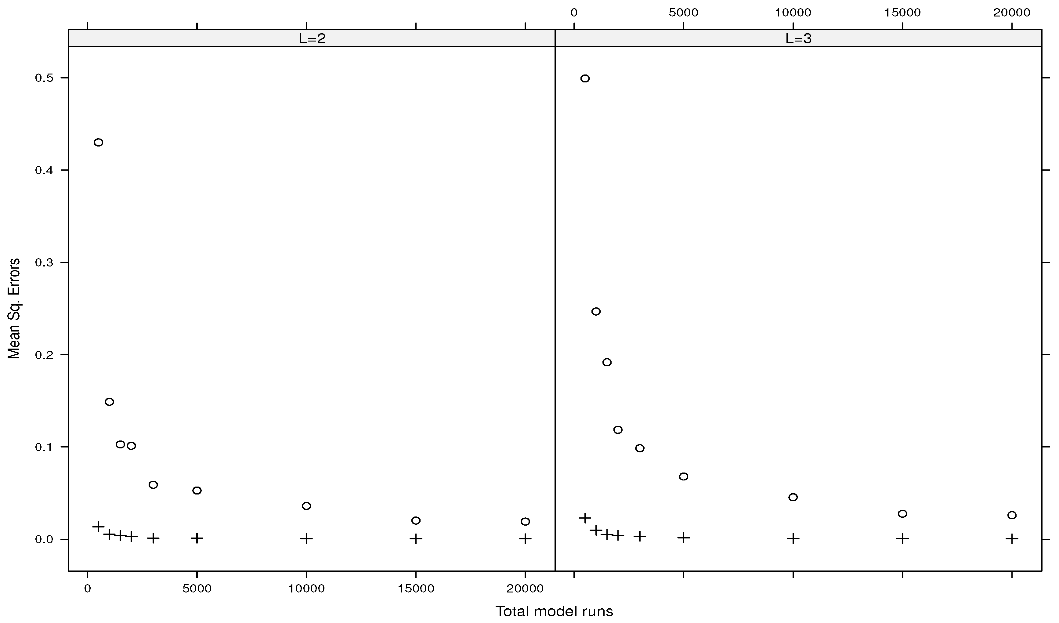
Figure 3.
Average of mean squared errors using the g-function of type B (○ the direct estimator (16) and + for the plug-in estimator (18)).
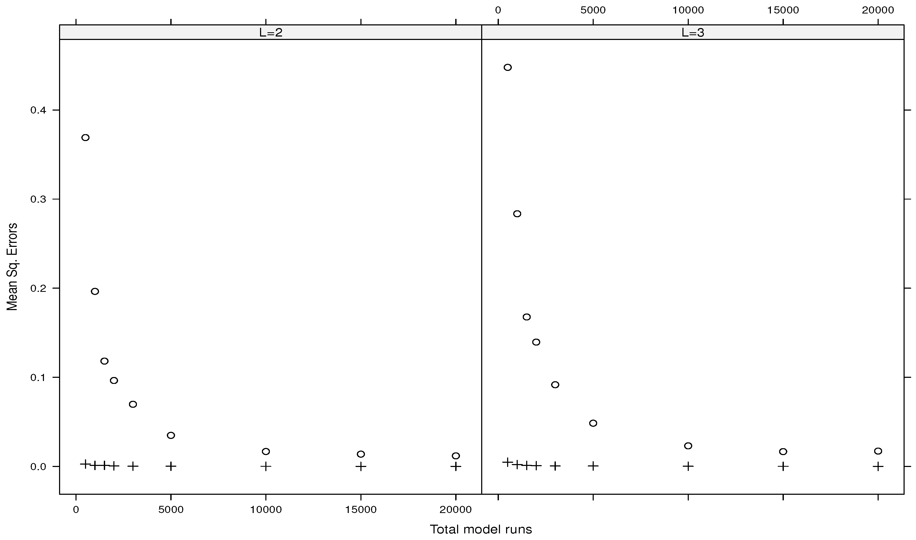
Figure 4.
Average of mean squared errors using the g-function of type C (○ the direct estimator (16) and + for the plug-in estimator (18)).
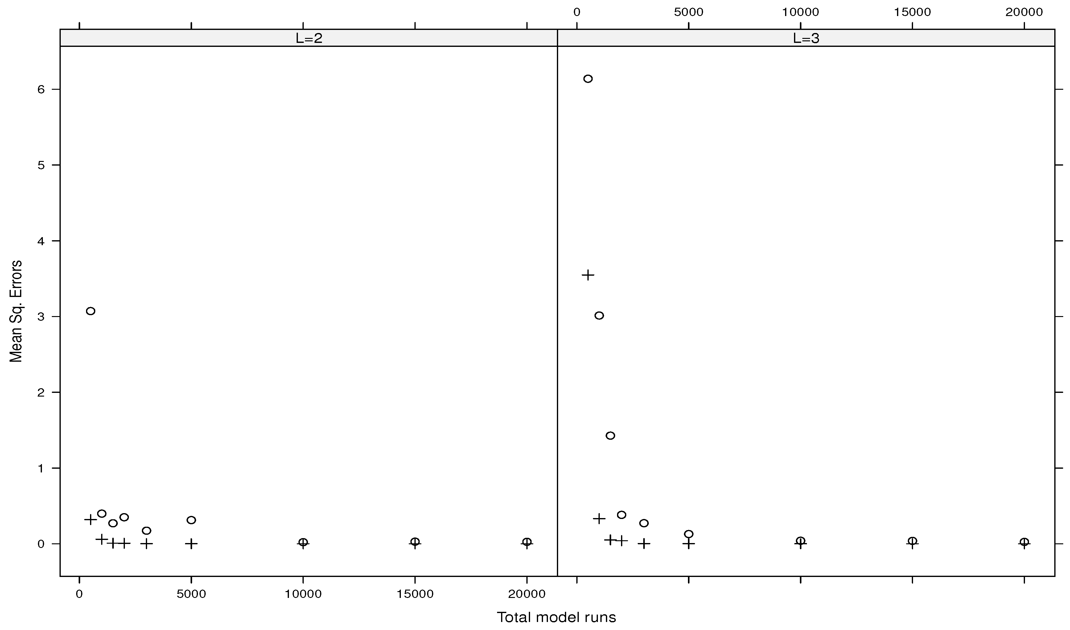
Figure 5.
Average of mean squared gaps using the Ishigami function (○ the direct estimator (17) and + for the plug-in estimator (19)).

Figure 6.
Average of mean squared gaps using the g-function of type A (○ the direct estimator (17) and + for the plug-in estimator (19)).
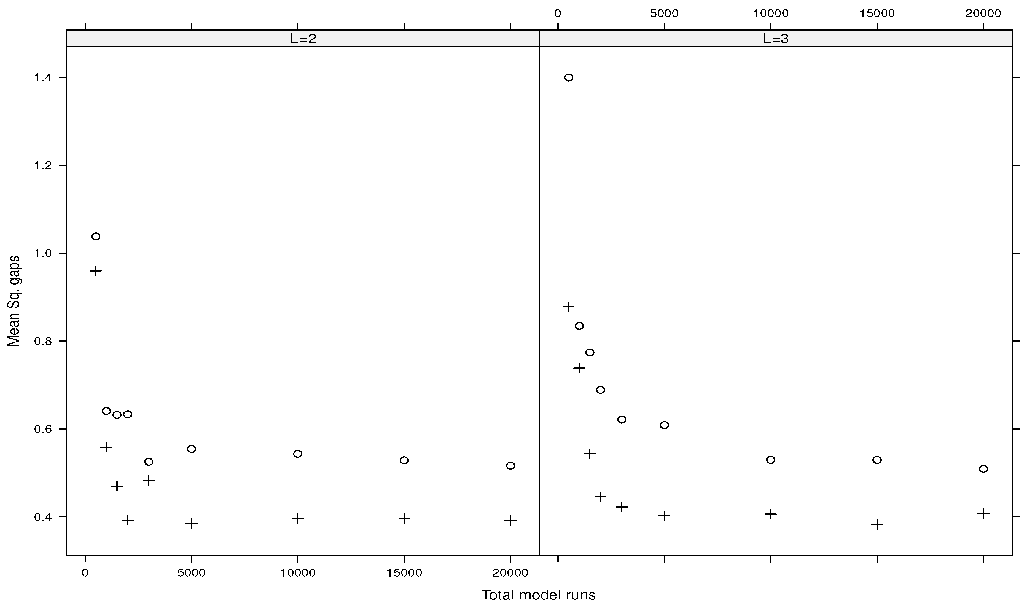
Figure 7.
Average of mean squared gaps using the g-function of type B (○ the direct estimator (17) and + for the plug-in estimator (19)).
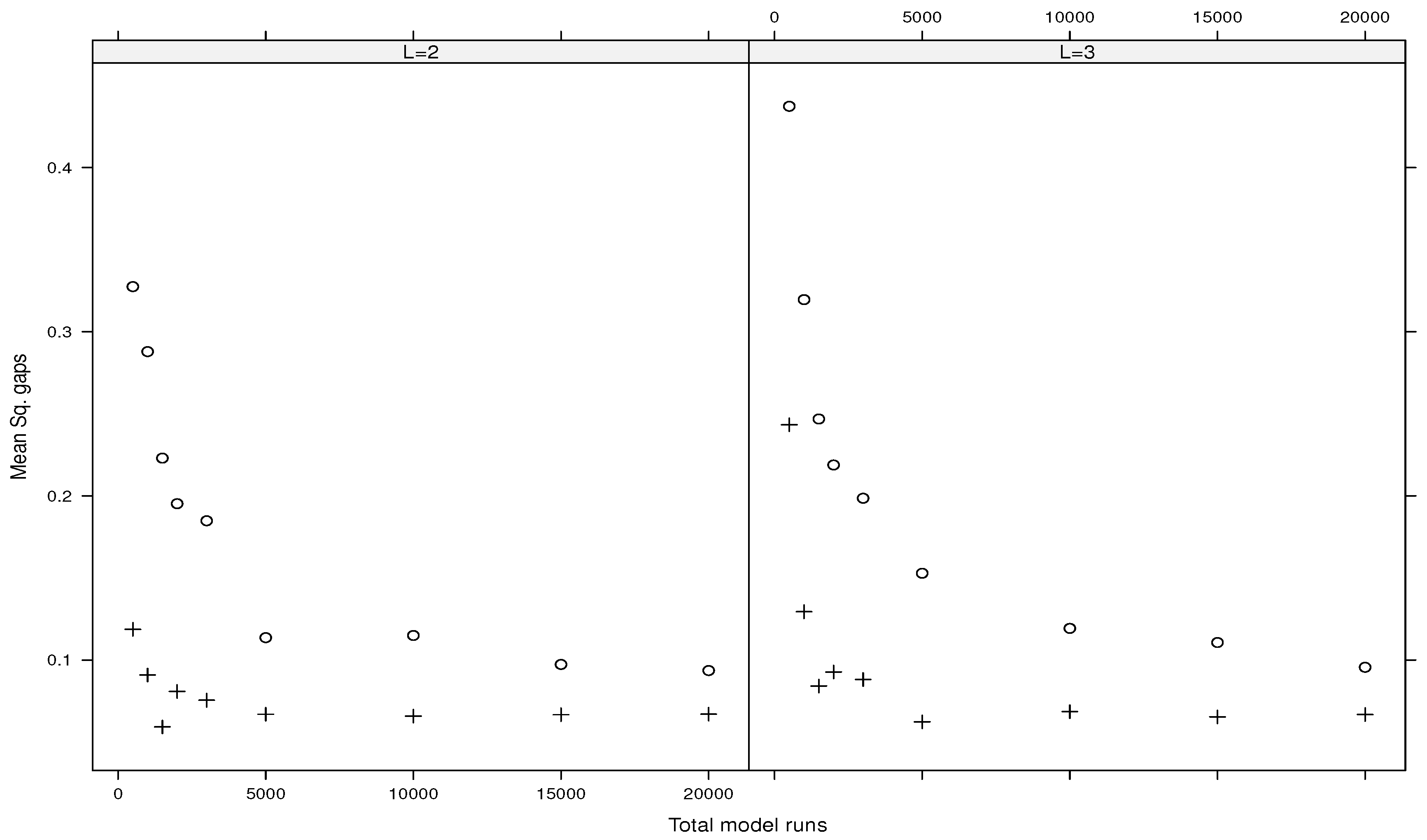
Figure 8.
Average of mean squared gaps using the g-function of type C (○ the direct estimator (17) and + for the plug-in estimator (19)).

Figure 9.
Predictions of g-function of type B using the emulator versus observations using and .

Table 1.
Average of 30 estimates of the main indices and upper bounds of total indices for the Ishigami function using the plug-in estimators, , and 2000 model runs.
Table 1.
Average of 30 estimates of the main indices and upper bounds of total indices for the Ishigami function using the plug-in estimators, , and 2000 model runs.
| X1 | X2 | X3 | |
|---|---|---|---|
| 0.249 | 0.318 | −0.006 | |
| 1.420 | 4.872 | 0.711 |
Table 2.
Average of 30 estimates of the main indices and upper bounds of total indices for the g-functions using the plug-in estimators, , and 2000 model runs.
Table 2.
Average of 30 estimates of the main indices and upper bounds of total indices for the g-functions using the plug-in estimators, , and 2000 model runs.
| X1 | X2 | X3 | X4 | X5 | X6 | X7 | X8 | X9 | X10 | |
|---|---|---|---|---|---|---|---|---|---|---|
| Type A | ||||||||||
| 0.330 | 0.324 | 0.006 | 0.005 | 0.006 | 0.006 | 0.005 | 0.005 | 0.006 | 0.005 | |
| 2.022 | 2.005 | 0.045 | 0.046 | 0.047 | 0.047 | 0.046 | 0.046 | 0.046 | 0.047 | |
| Type B | ||||||||||
| 0.085 | 0.085 | 0.085 | 0.085 | 0.085 | 0.085 | 0.085 | 0.085 | 0.085 | 0.085 | |
| 0.362 | 0.363 | 0.363 | 0.362 | 0.363 | 0.362 | 0.363 | 0.362 | 0.363 | 0.363 | |
| Type C | ||||||||||
| 0.028 | 0.028 | 0.032 | 0.032 | 0.035 | 0.041 | 0.031 | 0.030 | 0.036 | 0.034 | |
| 2.033 | 1.301 | 1.825 | 1.605 | 1.634 | 1.641 | 2.216 | 1.526 | 1.793 | 1.503 | |
Disclaimer/Publisher’s Note: The statements, opinions and data contained in all publications are solely those of the individual author(s) and contributor(s) and not of MDPI and/or the editor(s). MDPI and/or the editor(s) disclaim responsibility for any injury to people or property resulting from any ideas, methods, instructions or products referred to in the content. |
© 2024 by the author. Licensee MDPI, Basel, Switzerland. This article is an open access article distributed under the terms and conditions of the Creative Commons Attribution (CC BY) license (https://creativecommons.org/licenses/by/4.0/).
Share and Cite
MDPI and ACS Style
Lamboni, M. Optimal Estimators of Cross-Partial Derivatives and Surrogates of Functions. Stats 2024, 7, 697-718. https://doi.org/10.3390/stats7030042
AMA Style
Lamboni M. Optimal Estimators of Cross-Partial Derivatives and Surrogates of Functions. Stats. 2024; 7(3):697-718. https://doi.org/10.3390/stats7030042
Chicago/Turabian StyleLamboni, Matieyendou. 2024. "Optimal Estimators of Cross-Partial Derivatives and Surrogates of Functions" Stats 7, no. 3: 697-718. https://doi.org/10.3390/stats7030042