Limits of Agreement Based on Transformed Measurements

Abstract

Method comparison studies are typically analyzed using limits of agreement (LoAs). The standard Bland–Altman approach estimates LoAs under the assumption that the differences between methods follow a normal distribution. However, many types of measurements, such as volume, concentration, and percentage values, often deviate from normality. This study explores LoAs for the difference between two clinical measurements and prediction intervals for one measurement given the other, using a transformation of the data. After back-transforming, the resulting LoA for the original measurements depends on the subject level, represented by the average of the measurements. A simulation study evaluates the statistical properties of these LoAs and their confidence limits, demonstrating strong performance for small-to-medium sample sizes. LoA derived from transformed measurements are also compared with those obtained using a regression-based method proposed by Bland and Altman. Two applications demonstrate the approach using logarithmic and cube root transformations. This transformation-based method offers a straightforward way to obtain LoAs that depends on the subject level.

1. Introduction

Limits of agreement (LoAs) are a central part of comparing measurement methods and replications of the same method. An LoA assesses limits for a future difference between two methods or measurements. The standard analysis, often called the Bland–Altman analysis, is to plot the difference against the average to ensure that the distribution of difference does not depend on the subject level [1]. A quantile–quantile plot of the differences is useful to ensure normality of the differences. The LoA is then estimated as the central 95% range of the normal distribution with the same mean and standard deviation. In principle, the central range may also be estimated non-parametrically, but the non-parametric LoA requires a much larger sample to determine the 2.5 and 97.5 percentile of the differences. In some cases, the model assumptions are derived from a logarithmic transformation of the measurements and then the LoA for the log-transformed measurements can be back-transformed into the LoA for the ratio of measurements [1]. The LoA based on absolute differences or the ratio using log-transformation is the only way to obtain one LoA value valid for all subjects. Many clinicians, however, find the LoA of the absolute differences much easier to interpret than the LoA of ratios.

Bland–Altman considered creating LoAs that depend on the subject level by using one or two linear regressions of the difference against a function of the average of the measurements [2]. LoAs can then be derived from the linear regression models. It may, however, be difficult to find the appropriate regression model. This regression method has, for example, been used to compute LoAs for coronary artery calcium measurements reported in several papers [3,4,5]. The Agatston score describes the volume of calcified plaque inside the walls of the cardiac arteries. Here, the function of the average to model the standard deviation dependency was found using fraction polynomials and statistical significance testing. In some of these applications, the LoA seems to fit less well for the smaller measurements [5].

Lise Brøndsted suggested in her PhD dissertation to create a subject-dependent LoA based on a transformation of the measurements in the case of percentage measurements and using the logit-transformation [6]. An illustration of this method with percentage measurements and the logit-transformation was presented by Carstensen [7]. The statistical uncertainty of these limits were, however, not discussed. To the best of our knowledge, the suggestion of Lise Brøndsted has rarely been used in clinical practice.

Frank Harrell, among others, suggests to use a dimensionality argument for the choice of transformation of outcome data, exemplified by a cube root transformation of volume measurements or per unit of volume counts like blood cell counts [8]. The cube root transformation accounts for random variation across the three dimensions of volume. With the same argument, one should use the square root transformation when the measurements include area or counts in the plane; for example, cell counts viewed in a microscope. For concentration measurements, the logarithmic function is often used, and for percent measurements the logarithmic or logit function are frequently applied. The transformation can sometimes be selected to stabilize the variance [9].

This paper provides a detailed discussion on Lise Brøndsted’s suggestion of estimating the LoA through a transformation of the measurements. This study presents an alternative way of computing the LoA, which also yields a way of quantifying its statistical uncertainty. The statistical properties are studied in a simulation study. Similarly, a prediction interval of one measurement given the other measurement is presented, which can be placed on a scatter plot of one measurement against the other. Furthermore, a connection is established between the LoA based on a transformation of the measurements and the LoA derived from the regression method proposed by Bland–Altman [2]. The two applications that motivated the current study are presented: sperm DNA fragmentation index using a logarithmic transformation and coronary plaque volume measurements using a cube root transformation. This paper contributes to the existing literature by illustrating the use of cube root transformation for volume data. Additionally, this paper discusses the quantification of the statistical uncertainty of the transformed LoA and establishes the connection to the regression method proposed by Bland–Altman.

2. Method

2.1. Standard Limits of Agreement

The standard Bland–Altman model [1] is reviewed in the following section. Consider measurements $y_{mi}$ by method $m=1,2$ that aims at measuring the true subject level ${\mu }_i$ on subjects $i=1,\dots ,n$. The measurements are assumed to satisfy the normal model

$$\begin{array}{c}\hfill y_{mi}={\alpha }_m+{\mu }_i+e_{mi},\end{array}$$

(1)

where $e_{mi}\sim \mathrm{N}(0,{\sigma }_m^2)$. The ${\alpha }_m$ is the mean difference and $e_{mi}$ is the random difference from the true level ${\mu }_i$ when performing measurement by method m on the subject i. The model assumes that the mean difference between the two measurements is independent of the subject level. Under this assumption, the mean difference is given by ${\alpha }_1-{\alpha }_2$. Additionally, the model assumes that the measurement precision, ${\sigma }_m$, remains constant across all subjects. Let $D_i=y_{1i}-y_{2i}$ and $A_i=(y_{1i}+y_{2i})/2$ denote the difference and average of the subject measurements. Prediction limits for the difference between measurements for a (future) measurement, $D_0$, is based on $D_0\sim \mathrm{N}({\alpha }_1-{\alpha }_2,{\sigma }_1^2+{\sigma }_2^2)$. The mean difference ${\alpha }_1-{\alpha }_2$ is estimated by the sample average $\overline{D}={\displaystyle \frac{1}{n}}{\sum }_{i=1}^n{D}_i$ and the variance ${\sigma }_D^2={\sigma }_1^2+{\sigma }_2^2$ by the empirical variance ${\widehat{\sigma }}_D^2={\displaystyle \frac{1}{n-1}}{\sum }_{i=1}^n{(D_i-\overline{D})}^2$. The estimated LoA is then

$$\begin{array}{c}\hfill \overline{D}\pm 1.96·{\widehat{\sigma }}_D.\end{array}$$

(2)

The LoA estimates the central 95% of all differences between the two measurements based on the normal model, providing a quantification of how closely the measurements agree. The mean and variance of the differences are assumed to be constant over the range of measurements. This is evaluated in the so-called Bland–Altman plot of the differences against the average, where the average of the measurements is used as the best estimate of the true value. Often, the LoA is added to this plot. When the Bland–Altman plot shows a relationship between the difference and average of measurements it does not necessarily imply that there is a relationship between the difference and the true subject value. It may also be due to the fact that the average of the measurements is used as the best estimate of the true value. A correlation in the Bland–Altman plot may occur if the variation of the two methods are different [10]. However, if the measurements are evaluated over a wide range of subjects, then the within-subject variance of the measurements is then only a small part of the total variance of the measurements, and then only a weak correlation will appear in the Bland–Altman plot due to difference of measurement precision [11]. When replications of the same method are performed, the measurements will have same precision and then a correlation in the Bland–Altman plot is due to an association between the measurement error and the true value.

The LoA in (2) considers the estimated model as fixed when predicting a future observation. If the model uncertainty is taken into account, then the factor $1.96$ should be replaced by a 97.5 percentile in a t-distribution with $n-1$ degrees of freedom. Often, however, the factor $1.96$ is replaced by 2 as a simple way of compensating for the model uncertainty [7]. The confidence interval of the mean difference is based on the t-distribution with $n-1$ degrees of freedom and the standard error $\mathrm{se}\left(\overline{D}\right)={\sigma }_D/\sqrt{n}$. The approximate confidence interval for the LoA can be derived from the standard error [2]

$$\begin{array}{c}\hfill \mathrm{se}={\sigma }_D·\sqrt{1/n+1.{96}^2/(2n-2)}.\end{array}$$

(3)

Other methods for obtaining the confidence limits, including an exact method based on the non-central t-distribution, are discussed by Shieh [12]. In the case when the measurements can be considered exchangeable, so that the mean difference is zero, the LoA is given by $\pm 1.96·{\widehat{\sigma }}_{D0}$, where ${\widehat{\sigma }}_{D0}^2={\displaystyle \frac{1}{n}}{\sum }_{i=1}^n{D}_i^2$, and exact confidence limits for the LoA can here be derived from the ${\chi }^2$-distribution with n degrees of freedom. The limits of agreement (LoAs) represent the range that captures the central 95% of the observed differences between measurements. In contrast, the confidence interval for the LoA quantifies the uncertainty in the estimated LoA limits, indicating how precisely they have been determined.

A prediction interval for a future measurement by method 2, $y_{20}$, when a measurement of method 1 is performed, $y_{10}$, is computed by first deriving ${\mu }_0=y_{10}-{\alpha }_1-e_{10}$ from the first measurement model and inserting this in the model for the second measurement [13]

$$\begin{array}{cc}\hfill y_{20}& ={\alpha }_2+{\mu }_0+e_{20}\hfill \\ \hfill & =y_{10}+{\alpha }_2-{\alpha }_1+e_{20}-e_{10}.\hfill \end{array}$$

The $y_{10}$ measurement is considered fixed, whereas one uses $D_i={\alpha }_1-{\alpha }_2+e_{10}-e_{20}\sim \mathrm{N}({\alpha }_1-{\alpha }_2,{\sigma }_1^2+{\sigma }_2^2)$. The prediction interval is thus given as

$$\begin{array}{cc}\hfill \mathrm{PI}\left(y_{20}\right|y_{10})& =y_{10}-\overline{D}\pm 1.96·{\widehat{\sigma }}_D.\hfill \end{array}$$

(4)

The limits are often placed on the scatter plot of $(y_{m1},y_{m2})$. The reverse predicting is

$$\begin{array}{cc}\hfill \mathrm{PI}\left(y_{10}\right|y_{20})& =y_{20}+\overline{D}\pm 1.96·{\widehat{\sigma }}_D.\hfill \end{array}$$

(5)

It is easy to show that the two sets of prediction lines are the same, thus the prediction limits are applicable in both ways of the $(y_{m1},y_{m2})$ scatter plot.

The subject level ${\mu }_i$ is considered a fixed parameter corresponding to the intention to measure the subject’s true level; see also Carstensen [7]. However, the Bland–Altman analysis will not depend on whether the subject levels are considered fixed parameters or random effects. If one is willing to assume the same measurement precision of the two measurements, for example when the measurements are replications of the same method, then a comparison can also be made using a normal mixed model. In the mixed model, one furthermore assumes that the subject levels follow a normal distribution, although simulations show that the mixed model does not seem to be sensitive to correct specifications of random effect distribution [14]. When two or more replications of each method are available, then the mixed analysis can be performed without the assumption of the same measurement precision [15].

In situations where the mean or standard deviation of the difference depend on the true subject level, the most common approach has been a regression approach of Bland–Altman based on one or two linear regression models of the difference on some function of the average [2]. One standard linear regression model is applied on the difference on some function on the average to model the mean dependence on the subject levels. Another separate, linear regression model is applied on the absolute value of differences, or residuals from the first step linear regression, on some function of the average to model the standard deviation dependence of the subject levels. The second step is based the fact that the mean absolute value of a normal distribution is $\sqrt{2/\pi }$ times the standard deviation of the normal distribution. LoAs can then be derived from the linear regression models. The statistical uncertainty of these LoAs involving the second linear regression is less clear. Carstensen described a regression method for measurement where the methods are related linearly to the true subject level, but the measurement precisions are assumed constant over the range of measurements [13]. Other solutions have also been described elsewhere [16,17]. Critiques of the Bland–Altman analysis appear in the literature [18,19]. Mansournia and colleagues argue thoroughly that the critique is due to the use of the Bland–Altman analysis outside the intention of the analysis to answer, ’Do the two methods of measurement agree sufficiently closely?’ [11].

2.2. Limits of Agreement Based on Transformed Measurements

Assuming that the same LoAs model holds for transformed measurements,

$$\begin{array}{c}\hfill \varphi \left(y_{mi}\right)={\alpha }_m+{\mu }_i+e_{mi},\end{array}$$

(6)

where $\varphi$ is some monotone function and $e_{mi}\sim \mathrm{N}(0,{\sigma }_m^2)$. Let $D_{\varphi i}=\varphi \left(y_{1i}\right)-\varphi \left(y_{2i}\right)$ and $A_{\varphi i}=(\varphi \left(y_{1i}\right)+\varphi \left(y_{2i}\right))/2$ denote the difference and average on the transformed scale and maintain $D_i=y_{1i}-y_{2i}$ and $A_i=(y_{1i}+y_{2i})/2$ as the difference and average on the untransformed scale. As above, the mean difference ${\alpha }_1-{\alpha }_2$ is estimated by the sample average ${\overline{D}}_{\varphi }={\displaystyle \frac{1}{n}}{\sum }_{i=1}^n{D}_{\varphi i}$, the variance ${\sigma }_{D\varphi }^2={\sigma }_1^2+{\sigma }_2^2$ by the empirical variance ${\widehat{\sigma }}_{D\varphi }^2={\displaystyle \frac{1}{n-1}}{\sum }_{i=1}^n{(D_{\varphi i}-{\overline{D}}_{\varphi })}^2$, and the LoA on the transformed scale by

$$\begin{array}{c}\hfill {\mathrm{LoA}}_{\varphi }:{\widehat{\alpha }}_1-{\widehat{\alpha }}_2\pm 1.96·{\widehat{\sigma }}_{D\varphi }.\end{array}$$

(7)

Carstensen [7] described a back-transformed LoA for the original measurements in an example for percent measurements, where $\varphi$ is the logit function: Generate a sequence of x values and make the transformation of these by $\varphi \left(x\right)$. Here, x is used for the $y_{1i}$ measurements and y for the $y_{2i}$ measurements. Then, generate transformed values $\varphi \left(y\right)$ using

$$\begin{array}{c}\hfill \varphi \left(y\right)=\varphi \left(x\right)-L,\end{array}$$

where L is one of the ${\mathrm{LoA}}_{\varphi }$ limits, and back-transform these to the original y scale by

$$\begin{array}{c}\hfill y={\varphi }^{-1}(\varphi \left(x\right)-L),\end{array}$$

(8)

creating limits that can be plotted on the $(y_{m1},y_{m2})$ plot. The LoAs plot is created by taking $(x,y)$ described by (8) and replacing them by $\left(\right(x+y)/2,x-y)$, plotting

$$\begin{array}{c}\hfill ({\displaystyle \frac{x+\varphi ({\varphi }^{-1}\left(x\right)-L)}{2}},x-\varphi ({\varphi }^{-1}\left(x\right)-L)).\end{array}$$

(9)

A similar transformation can be obtained for the mean difference estimated by ${\overline{D}}_{\varphi }$ to produce a median difference curve on the original scale. To find the LoA$\left(a\right)$ for a given average, e.g., a, requires searching for the first component of (9) closest to a. It is not clear how the statistical uncertainty of these estimates should be derived and the statistical uncertainty was not discussed by Carstensen.

The statistical uncertainty can be derived from reformulating the back-transformed LoA. The above method essentially defines the back-transformed LoA as

$$\begin{array}{c}\hfill (x-y)\in \mathrm{LoA}((x+y)/2)\mathrm{if}\varphi \left(x\right)-\varphi \left(y\right)\in {\mathrm{LoA}}_{\varphi }.\end{array}$$

It is convenient to write this in terms of the average and difference of the original measurements, $(a,d)=\left(\right(x+y)/2,x-y)$,

$$\begin{array}{c}\hfill \mathrm{LoA}\left(a\right)=\{d:\varphi (a+d/2)-\varphi (a-d/2)\in {\mathrm{LoA}}_{\varphi }\},\end{array}$$

(10)

where it is used that $x=a+d/2$ and $y=a-d/2$. For positive measurements, $a+d/2>0$ and $a-d/2>0$, suggesting that $-2a<d<2a$. The $\mathrm{LoA}\left(a\right)$ in (10) is thus defined in terms of the mapping

$$\begin{array}{c}\hfill {\mathrm{\Psi }}_a\left(d\right)=\varphi (a+d/2)-\varphi (a-d/2),\end{array}$$

(11)

which has the derivative

$$\begin{array}{c}\hfill {\mathrm{\Psi }}_a^{\prime }\left(d\right)={\displaystyle \frac{1}{2}}{\varphi }^{\prime }(a+d/2)+{\displaystyle \frac{1}{2}}{\varphi }^{\prime }(a-d/2).\end{array}$$

If $\varphi$ is an increasing function, then (11) is also increasing.

The requirement for determining (10) can be addressed by solving the following equation for d, with a fixed a:

$$\begin{array}{c}\hfill {\mathrm{\Psi }}_a\left(d\right)=\varphi (a+d/2)-\varphi (a-d/2)=L,\end{array}$$

(12)

where L represents one of the limits of ${\mathrm{LoA}}_{\varphi }$ or its corresponding confidence limits. This formulation, as described in (12), is particularly advantageous because most statistical software packages provide effective equation solvers. Moreover, it defines $\mathrm{LoA}\left(a\right)$ as a mapping of ${\mathrm{LoA}}_{\varphi }$, which can be applied directly to the corresponding confidence limits. It follows that a confidence interval for ${\mathrm{LoA}}_{\varphi }$ with (approximate) 95% coverage for the transformed measurements will be back-transformed into a confidence interval for $\mathrm{LoA}\left(a\right)$ with (approximate) 95% coverage.

In the special case where $\varphi \left(x\right)=log\left(x\right)$, the LoA can be back-transformed into a ratio between the measurements [1]. However, often clinicians are more interested in an absolute comparison rather then the relative comparison. The equation

$$\begin{array}{c}\hfill log(a+d/2)-log(a-d/2)=L\end{array}$$

has the solution

$$\begin{array}{c}\hfill d=-2·{\displaystyle \frac{1-exp\left(L\right)}{1+exp\left(L\right)}}·a.\end{array}$$

Here, the LoAs for the absolute difference are linear functions of the average.

For the square root and cube root transformations, the LoA in (9) is given by

$$\begin{array}{cc}\hfill \varphi \left(x\right)=x^{{\displaystyle \frac{1}{2}}}:& ({\displaystyle \frac{x+{(x^2-L)}^{1/2}}{2}},x-{(x^2-L)}^{1/2})\hfill \\ \hfill \varphi \left(x\right)=x^{{\displaystyle \frac{1}{3}}}:& ({\displaystyle \frac{x+{(x^3-L)}^{1/3}}{2}},x-{(x^3-L)}^{1/3}).\hfill \end{array}$$

A prediction interval for a future measurement by method 2, $y_{20}$, when a measurement of method 1 is performed, $y_{10}$, is computed by first deriving ${\mu }_0=\varphi \left(y_{10}\right)-{\alpha }_1-e_{10}$ from the first measurement and inserting this in the model for the second measurement

$$\begin{array}{cc}\hfill y_{20}& ={\varphi }^{-1}(\varphi \left(y_{10}\right)+{\alpha }_2-{\alpha }_1+e_{20}-e_{10}),\hfill \end{array}$$

resulting in the prediction interval

$$\begin{array}{cc}\hfill \mathrm{PI}\left(y_{20}\right|y_{10})& ={\varphi }^{-1}(\varphi \left(y_{10}\right)-{\overline{D}}_{\varphi }\pm 1.96·{\widehat{\sigma }}_{D\varphi }).\hfill \end{array}$$

(13)

The reverse predicting interval is

$$\begin{array}{cc}\hfill \mathrm{PI}\left(y_{10}\right|y_{20})& ={\varphi }^{-1}(\varphi \left(y_{20}\right)+{\overline{D}}_{\varphi }\pm 1.96·{\widehat{\sigma }}_{D\varphi }).\hfill \end{array}$$

(14)

It can be shown that the two sets of prediction curves are the same, thus the prediction limits are also here applicable both ways in the $(y_{m1},y_{m2})$ scatter plot. The prediction interval for a follow-up measurement is important in clinical practice during an intervention, as it determines the magnitude of difference between the first and second measurements needed to attribute the change to the intervention. This is further discussed in the sperm DNA fragmentation index example presented in Section 4.1.

The equation identifying the LoA in (12) has at most one solution if $\varphi$ is either increasing or decreasing. However, there may not always be a solution. Our empirical experience for positive measurements is that this may happen for small values of the average. A pragmatic solution is here to take the value of −2a and 2a closest to 0 in (12). In contrast, the prediction limits of one measurement given the other measurement in (14) and (13) are always well defined.

3. Simulations

The simulations illustrate for $\varphi =log\left(x\right)$ the coverage of LoA$\left(a\right)$ and its confidence limits CI (Lower LoA$\left(a\right)$) and CI (Upper LoA$\left(a\right)$) at a pre-specified value of the average compared to the coverage of ${\mathrm{LoA}}_{\varphi }$ and its confidence limits CI (Lower ${\mathrm{LoA}}_{\varphi }$) and CI (Upper ${\mathrm{LoA}}_{\varphi }$). The set-up is chosen to match the DFI data presented in Section 4.1 using model (6) for the outcome data on the logarithmic scale. The distribution of ${\mu }_i$ between subjects is assumed to follow a normal distribution with between-subject standard deviation ${\mathrm{sd}}_{\mathrm{b}}$ = 0.62 and ${\sigma }_{\mathrm{m}}=\mathrm{Ratio}·{\mathrm{sd}}_{\mathrm{b}}$ with Ratio = 0.25, 0.50, 1.00. The Ratio = 0.25 corresponds to the estimated measurement standard deviation ${\mathrm{sd}}_{\mathrm{m}}$ in the DFI data. The purpose of varying the between-subject variance ${\mathrm{sd}}_{\mathrm{b}}$ is to evaluate the robustness of using the average of the two measurements as an estimate of the true subject level. The median difference in the original measurements is set to 17.4% as in the DFI data and the pre-specified average is set to 20%. The ${\mathrm{LoA}}_{\varphi }$, LoA$\left(a\right)$, and associated confidence limits are estimated based on $n=50,100,200,$ and 500 observations and the coverage is evaluated with 10,000 replications. The coverage of LoA$\left(a\right)$ is based on the conditional distribution $Pr(·|A=a)$, which is simulated using a rejection algorithm, where the simulated average was allowed to differ from the pre-specified 20% within an error margin of 0.1%.

Table 1. Coverage of ${\mathrm{LoA}}_{\varphi }$, LoA$\left(a\right)$, and confidence limits based on a log-normal model.

				Coverage
				${\mathbf{LoA}}_{\mathit{\varphi }}$			LoA$\left(\mathbf{a}\right)$
$\mathbf{n}$	Ratio	${\mathbf{sd}}_{\mathbf{b}}$	${\mathbf{sd}}_{\mathbf{m}}$	${\mathbf{LoA}}_{\mathit{\varphi }}$	CI (Lower)	CI (Upper)	LoA$\left(\mathbf{a}\right)$	CI (Lower)	CI (Upper)
50	0.25	0.62	0.16	0.905	0.936	0.937	0.905	0.936	0.937
50	0.50	0.62	0.31	0.903	0.939	0.946	0.898	0.939	0.946
50	1.00	0.62	0.62	0.952	0.942	0.937	0.959	0.942	0.937
100	0.25	0.62	0.16	0.964	0.944	0.945	0.961	0.944	0.945
100	0.50	0.62	0.31	0.938	0.951	0.947	0.941	0.951	0.947
100	1.00	0.62	0.62	0.941	0.948	0.947	0.946	0.948	0.947
200	0.25	0.62	0.16	0.925	0.948	0.950	0.924	0.948	0.950
200	0.50	0.62	0.31	0.947	0.946	0.947	0.944	0.946	0.947
200	1.00	0.62	0.62	0.918	0.947	0.946	0.922	0.947	0.946
500	0.25	0.62	0.16	0.963	0.952	0.949	0.959	0.952	0.949
500	0.50	0.62	0.31	0.955	0.950	0.949	0.958	0.950	0.949
500	1.00	0.62	0.62	0.949	0.951	0.952	0.952	0.951	0.952

shows that the coverage of LoA$\left(a\right)$ is similar to ${\mathrm{LoA}}_{\varphi }$. The coverage of the confidence limits for LoA$\left(a\right)$ is very similar to the coverage of confidence limits of ${\mathrm{LoA}}_{\varphi }$. The coverage did not seem to depend on the ratio between ${\mathrm{sd}}_{\mathrm{b}}$ and ${\mathrm{sd}}_{\mathrm{m}}$.

The Bland–Altman Regression Model

The presented $\mathrm{LoA}\left(a\right)$ is connected to the suggestion by Bland and Altman based on regression models, although the two LoAs are based on different model assumptions [2]: The Bland–Altman regression model assumes normality of the absolute difference, whereas the transformed LoA assumes normality of the transformed scale. In the regression method for the standard deviation, the absolute of a normal distribution has mean $\sqrt{2/\pi }·{\sigma }_D$, where ${\sigma }_D$ is the standard deviation of the difference. For positive measurements, the intercept is often chosen to be zero, so the standard deviation tends to zero when the function of A tends to zero. The standard deviation of D as function of A can then be obtained from the regression analysis and used to compute the LoA. Finding the right function of the average for the standard deviation analysis may, however, in practice be difficult since the standard residual method for the linear regression models does not apply.

Figure 1 shows simulated data corresponding to the coronary plaque volume measurements example. Simulated data are used to increase the sample size to promote comparison of the models. The left panel A presents linear regression of the absolute difference against the average (Identity); square root of the average (Square root); cube root of the average (Cube root); and the 2/3 root of the average, with the corresponding LoA in panel B. The identity seems to be too narrow for low values of the average and too wide for large values of the average. The opposite is seen for the square root and cube root, and both methods produce LoAs exceeding $\pm 2$ times the average range for small values of the average. The 2/3 root seems to give reasonable LoAs, but it is not clear from panel A why this function of the average should produce better LoAs. The residual standard deviation for the identity is 9.4; for the square root it is 8.9; for the cube root 9.3; and for the 2/3 root 8.8. Thus, the square root and 2/3 root have approximately the same squared distance of the observation to the mean line in panel A. It is shown below that the 2/3 root can be chosen based on a dimensionality argument for volume data, where the cube root transformation is a natural choice.

An approximate back-transformed LoA based on (7) can be derived using a Taylor expansion

$$\begin{array}{c}\hfill \varphi \left(y\right)-\varphi \left(x\right)={\varphi }^{\prime }\left(z\right)(y-x),\end{array}$$

where z is somewhere between x and y. Using the approximation $z\approx (x+y)/2=a$, it follows that

$$\begin{array}{c}\hfill \varphi \left(y\right)-\varphi \left(x\right)\approx {\varphi }^{\prime }\left(a\right)(y-x),\end{array}$$

implying that the mean difference and the LoAs of the transformed scale can be inverted to the original scale as

$$\begin{array}{cc}\hfill \mathrm{E}\left(D_i\right)& \approx {\displaystyle \frac{1}{{\varphi }^{\prime }\left(a\right)}}·\mathrm{E}\left(D_{\varphi i}\right)\hfill \\ \hfill \mathrm{LoA}\left(a\right)& \approx {\displaystyle \frac{1}{{\varphi }^{\prime }\left(a\right)}}·{\mathrm{LoA}}_{\varphi },\hfill \end{array}$$

suggesting that

$$\begin{array}{c}\hfill \mathrm{s}.\mathrm{d}.\left(D_i\right)\approx {\displaystyle \frac{1}{{\varphi }^{\prime }\left(a\right)}}·{\sigma }_{D\varphi }.\end{array}$$

Thus the transformation method implies an approximative structure for the Bland–Altman regression models for the both the mean and standard deviation in the case of the square root transformation $\mathrm{LoA}\left(a\right)\approx 2\sqrt{a}·{\mathrm{LoA}}_{\varphi }$; the cube root transformation $\mathrm{LoA}\left(a\right)\approx 3a^{2/3}·{\mathrm{LoA}}_{\varphi }$; and with the logarithmic function $\mathrm{LoA}\left(a\right)\approx a·{\mathrm{LoA}}_{\varphi }$. The dimensionality argument for the coronary plaque volume measurements thus suggests the 2/3 root transformation in the Bland–Altman regression method.

4. Applications

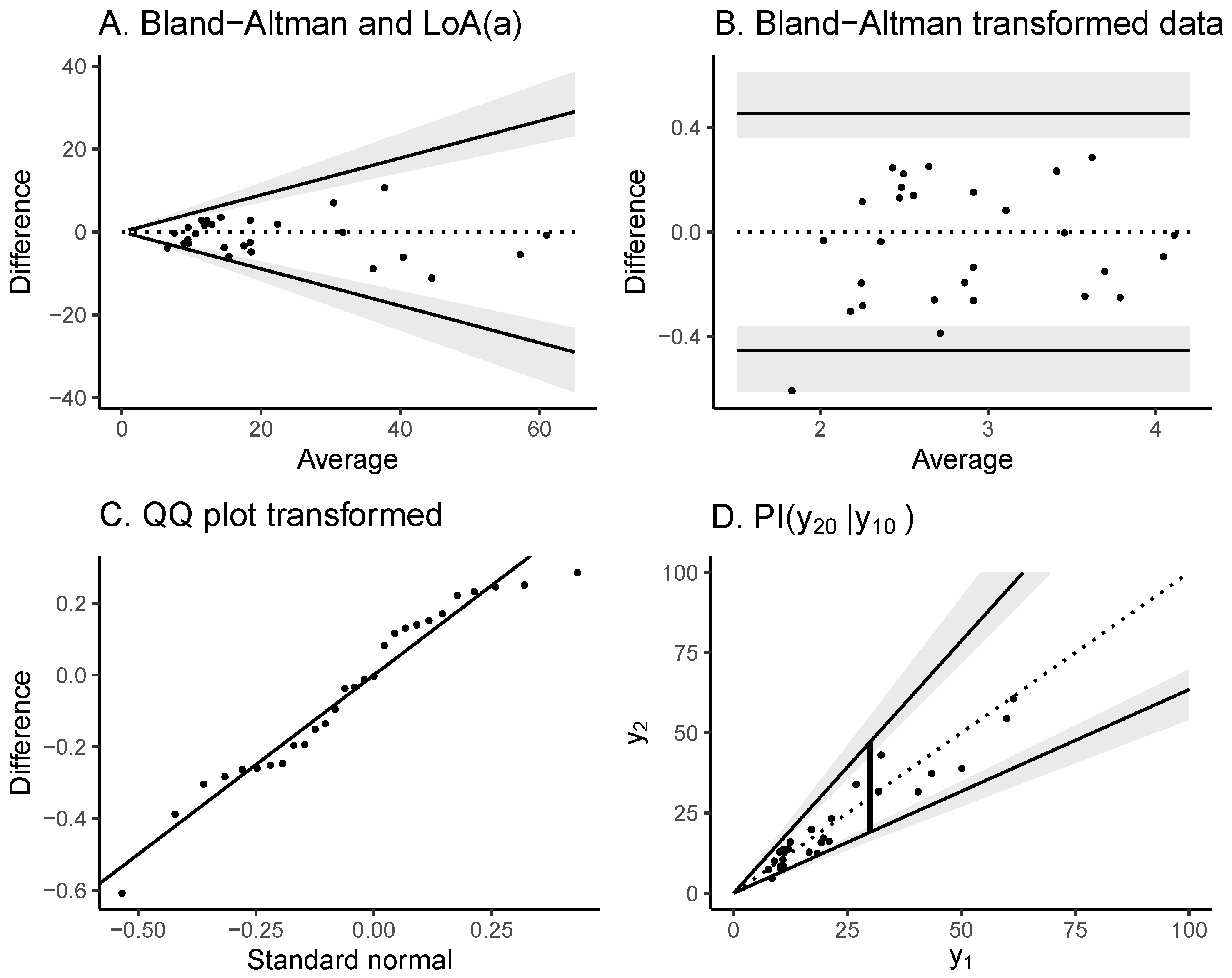
4.1. Sperm DNA Fragmentation Index

The sperm DNA fragmentation index (DFI) reflects the integrity of and the damage to the DNA of sperm cells and it is considered a crucial indicator to evaluate sperm quality. A high percentage DFI is associated with reduced fertility, early development of embryo, embryo quality, and pregnancy rates, and higher rates of spontaneous abortion [20]. The DFI depends on lifestyle factors including diet and exercise and is thus subject to lifestyle interventions. Often, DFI will be monitored over time. The following data on intra-male variation was accessed by two measurements made a few days apart involving 28 males at SPZ Lab.

The DFI closely follows a normal distribution on the logarithmic scale [21]. The Bland–Altman plots, LoA(a), and prediction interval PI($y_{20}$|$y_{10}$) are shown in Figure 2. The Bland–Altman plot (Figure 2, panel B) on the transformed measurements uses the assumption that the mean and variance of the differences are constant across the range of measurements. The quantile–quantile plot (Figure 2, panel C) uses the assumption of normality of the difference on the transformed scale. The Bland–Altman plot of the original data (Figure 2, panel A) shows the agreement of the measurements. The prediction interval for a follow-up measurement is used in clinical practice during lifestyle interventions aimed at reducing the DFI. It quantifies the magnitude of reduction in the DFI between the first and second measurements required to attribute the change to the intervention. For example, suppose a male has a DFI measurement of, e.g., 30%; the prediction interval of the second measurement is between 19.1% (95% CI: 16.2–20.9) and 47.2% (95% CI: 43.0–55.4%). Thus, a second measurement made after a lifestyle intervention should be lower than 19.1% (95% CI: 16.2–20.9) and claimed to be the result of the intervention (Figure 2, panel D).

The intra-male variation in DFI is relatively high, and there is an ongoing work to standardize the DFI measurements.

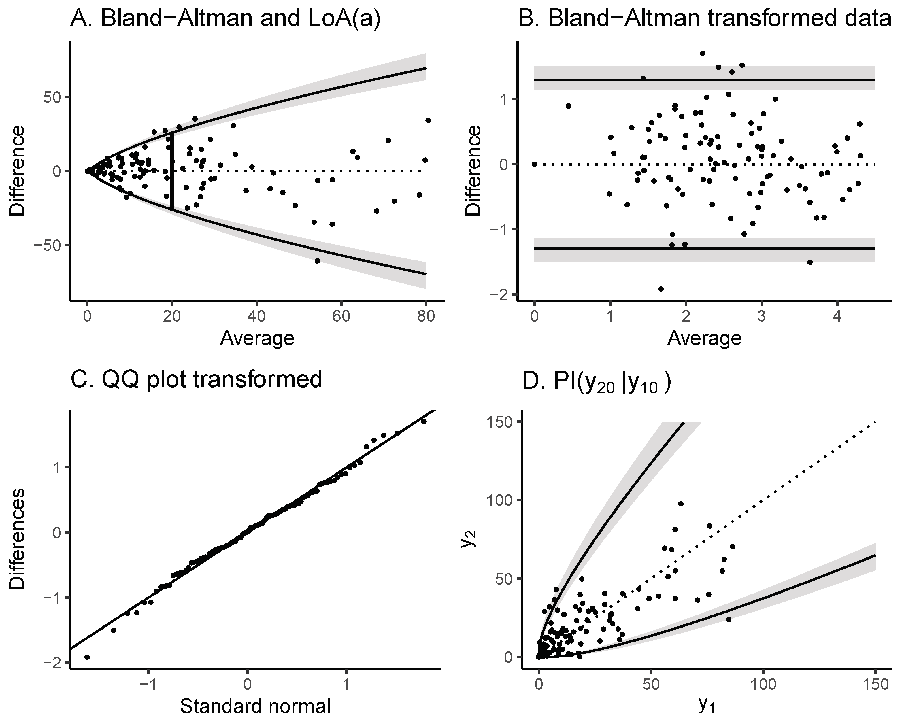
4.2. Coronary Plaque Volume Measurements

Iraqi and colleagues reported interscan reproducibility of computed tomography derived coronary plaque volume measurements using a semi-automated analysis software [22]. Computed-tomography-derived coronary plaque volume is a convenient way to measure coronary plaque in clinical practice. The coronary plaque volume measurements were performed twice in 101 consecutive patients with known coronary artery disease within a one-hour interval. The patients with known coronary artery disease form a homogeneous patient population. Coronary plaque volumes were quantified on a per-lesion and per-patient level and described as total plaque, non-calcified plaque, calcified plaque, and low-density non-calcified plaque. The focus here is on the low-density non-calcified plaque at the per-patient level. Figure 3 shows the Bland–Altman plots, LoA(a), and prediction interval PI($y_{20}$|$y_{10}$). The LoA at the average plaque volume of 20 is $\pm 26.0$ (95% CI: 23.4–29.2), thus the true LoA(20) is between $\pm 23.4$ and $\pm 29.2$. The LoA illustrates a modest reproducibility of the computed-tomography-derived coronary plaque volume measurements [22].

5. Discussion

This study presented prediction intervals of the difference in two clinical measurements, LoAs, and one measurement given the other measurement is observed based on a transformation of the measurements. Both intervals depend on the subject level represented by the average of the two measurements. The transformation can in many cases be chosen based on a dimensionality argument of the measurements, suggesting a specific functional form of the LoA as a function of the average. For strictly positive outcomes, the transformation can also be selected using the Box-Cox methodology [9]. The small and medium sample size properties of the LoAs and confidence intervals were evaluated in a simulation study. The presented LoAs were related to those proposed by Bland and Altman [2] using regression methods. The dimensionality argument suggests a specific transformation for both the mean and standard deviation model in the Bland–Altman regression models, which would also be a useful starting model for application of the Bland–Altman regression model.

Both the standard Bland–Altman method and the proposed transformation-based approach rely on a normality assumption. In principle, the limits of agreement (LoAs), defined as the central 95% range of measurement differences, could also be estimated using alternative parametric models.

The limits of agreement method assumes that the mean and variance of the differences remain constant across the range of measurements. This assumption is assessed using a Bland–Altman plot, which displays the differences against their averages. Additionally, it is assumed that the differences follow a normal distribution, evaluated using a quantile–quantile (QQ) plot. If the mean or variance of the differences varies across the range of measurements, alternative approaches, such as the regression method proposed by Bland and Altman [2] or Carstensen [13] can be applied. When comparing two measurement methods with two or more replications for each measurement, more advanced models, including the probability of agreement method [23], can be employed.

References

1. Bland, J.M.; Altman, D. Statistical methods for assessing agreement between two methods of clinical measurement. Lancet 1986, 327, 307–310. [Google Scholar] [CrossRef]
2. Bland, J.M.; Altman, D.G. Measuring agreement in method comparison studies. Stat. Methods Med. Res. 1999, 8, 135–160. [Google Scholar] [CrossRef] [PubMed]
3. Paixao, A.R.; Neeland, I.J.; Ayers, C.R.; Xing, F.; Berry, J.D.; de Lemos, J.A.; Abbara, S.; Peshock, R.M.; Khera, A. Defining coronary artery calcium concordance and repeatability-Implications for development and change: The Dallas Heart Study. J. Cardiovasc. Comput. Tomogr. 2017, 11, 347–353. [Google Scholar] [CrossRef] [PubMed]
4. Sevrukov, A.B.; Bland, J.M.; Kondos, G.T. Serial electron beam CT measurements of coronary artery calcium: Has your patient’s calcium score actually changed? Am. J. Roentgenol. 2005, 185, 1546–1553. [Google Scholar] [CrossRef] [PubMed]
5. Andersen, K.P.; Gerke, O. Assessing Agreement When Agreement Is Hard to Assess—The Agatston Score for Coronary Calcification. Diagnostics 2022, 12, 2993. [Google Scholar] [CrossRef]
6. Brøndsted, L. Quantification of Agreement. Ph.D. Thesis, Department of Biostatistics, University of Copenhagen, Copenhagen, Denmark, 2002. [Google Scholar]
7. Carstensen, B. Comparing Clinical Measurement Methods: A Practical Guide; John Wiley & Sons: Chichester, UK, 2011. [Google Scholar]
8. Harrell, F. Biostatistics for Biomedical Research. 2024. Available online: https://hbiostat.org/bbr/ (accessed on 26 March 2024).
9. Box, G.E.; Cox, D.R. An analysis of transformations. J. R. Stat. Soc. Ser. B Stat. Methodol. 1964, 26, 211–243. [Google Scholar] [CrossRef]
10. Bland, J.M.; Altman, D.G. Comparing methods of measurement: Why plotting difference against standard method is misleading. Lancet 1995, 346, 1085–1087. [Google Scholar] [CrossRef] [PubMed]
11. Mansournia, M.A.; Waters, R.; Nazemipour, M.; Bland, M.; Altman, D.G. Bland-Altman methods for comparing methods of measurement and response to criticisms. Glob. Epidemiol. 2021, 3, 100045. [Google Scholar] [CrossRef] [PubMed]
12. Shieh, G. The appropriateness of Bland-Altman’s approximate confidence intervals for limits of agreement. BMC Med. Res. Methodol. 2018, 18, 45. [Google Scholar] [CrossRef] [PubMed]
13. Carstensen, B. Comparing methods of measurement: Extending the LoA by regression. Stat. Med. 2010, 29, 401–410. [Google Scholar] [CrossRef] [PubMed]
14. McCulloch, C.E.; Neuhaus, J.M. Misspecifying the shape of a random effects distribution: Why getting it wrong may not matter. Statist. Sci. 2011, 26, 388–402. [Google Scholar] [CrossRef]
15. Carstensen, B. Comparing and predicting between several methods of measurement. Biostatistics 2004, 5, 399–413. [Google Scholar] [CrossRef]
16. Ludbrook, J. Confidence in Altman–Bland plots: A critical review of the method of differences. Clin. Exp. Pharmacol. Physiol. 2010, 37, 143–149. [Google Scholar] [CrossRef] [PubMed]
17. Francq, B.G.; Govaerts, B. How to regress and predict in a Bland–Altman plot? Review and contribution based on tolerance intervals and correlated-errors-in-variables models. Stat. Med. 2016, 35, 2328–2358. [Google Scholar] [CrossRef] [PubMed]
18. Hopkins, W. Bias in Bland-Altman but not regression validity analyses. Sportscience 2004, 8, 42–47. [Google Scholar]
19. Krouwer, J.S. Why Bland–Altman plots should use X, not (Y + X)/2 when X is a reference method. Stat. Med. 2008, 27, 778–780. [Google Scholar] [CrossRef]
20. Alahmar, A.T.; Singh, R.; Palani, A. Sperm DNA fragmentation in reproductive medicine: A review. J. Hum. Reprod. Sci. 2022, 15, 206–218. [Google Scholar] [CrossRef]
21. Christensen, P.; Fischer, R.; Schulze, W.; Baukloh, V.; Kienast, K.; Coull, G.; Parner, E.T. Role of intra-individual variation in the detection of thresholds for DFI and for misclassification rates: A retrospective analysis of 14,775 SCSA® tests. Andrology 2024, early view. [Google Scholar] [CrossRef]
22. Iraqi, N.; Mortensen, M.; Sand, N.; Busk, M.; Grove, E.; Dey, D.; Pedersen, K.; Kanstrup, H.; Madsen, K.; Parner, E.; et al. Interscan reproducibility of computed tomography derived coronary plaque volume measurements using a semi-automated analysis software. Eur. Heart J. 2024, 45, ehae666.175. [Google Scholar] [CrossRef]
23. Stevens, N.T.; Steiner, S.H.; MacKay, R.J. Assessing agreement between two measurement systems: An alternative to the limits of agreement approach. Stat. Methods Med. Res. 2017, 26, 2487–2504. [Google Scholar] [CrossRef] [PubMed]
Figure 1. Simulated volume data corresponding to the low-density non-calcified plaque (LD-NCP) volume in the coronary plaque volume measurements example. (A). Regression of the absolute difference against the average (Identity); square root of the average (Square root); cube root of the average (Cube root); and 2/3 root of the average (2/3 root). (B). LoAs corresponding to each of the four regression models.
Stats 08 00017 g001
Figure 2. DFI measurements: (A). Bland–Altman plot and LoAs on the original scale. (B). Bland–Altman plot and LoAs on log-transformed scale. (C). Quantile–quantile plot for log-transformed scale. (D). Prediction interval for one measurement given the other measurement is observed. The gray area shows the associated confidence intervals.
Stats 08 00017 g002
Figure 3. Coronary plaque volume measurements: (A). Bland–Altman plot and LoAs on the original scale. (B). Bland–Altman plot and LoAs on cube root-transformed scale. (C). Quantile–quantile plot for log-transformed scale. (D). Prediction interval for one measurement given the other measurement is observed. The gray area shows the associated confidence intervals.
Stats 08 00017 g003