
Bias-Corrected Fixed Item Parameter Calibration, with an Application to PISA Data


Abstract
1. Introduction
2. Bias Correction for DIF in Fixed Item Parameter Calibration
2.1. Maximum Likelihood Estimation in FIPC
2.2. Derivation of the Bias in FIPC
2.3. Bias-Corrected FIPC
2.4. Theoretical Results
2.5. Further Adaptations of FIPC and BCFIPC
2.6. Computation of Derivatives in BCFIPC
3. Simulation Study
3.1. Method
3.2. Results
4. Empirical Example: PISA 2006 Data
4.1. Method
4.1.1. Sample and Instruments
4.1.2. Sampling Weights and Standard Errors
4.1.3. Analysis
4.2. Results
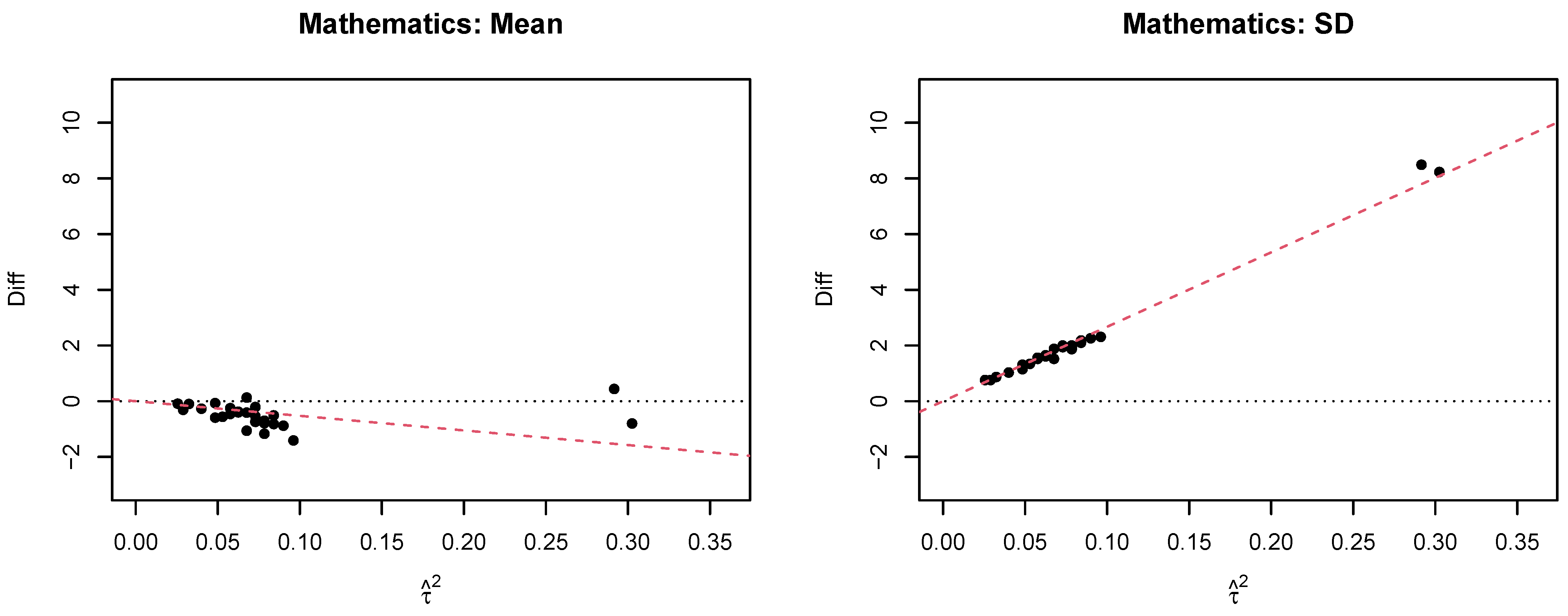
4.2.1. Mathematics
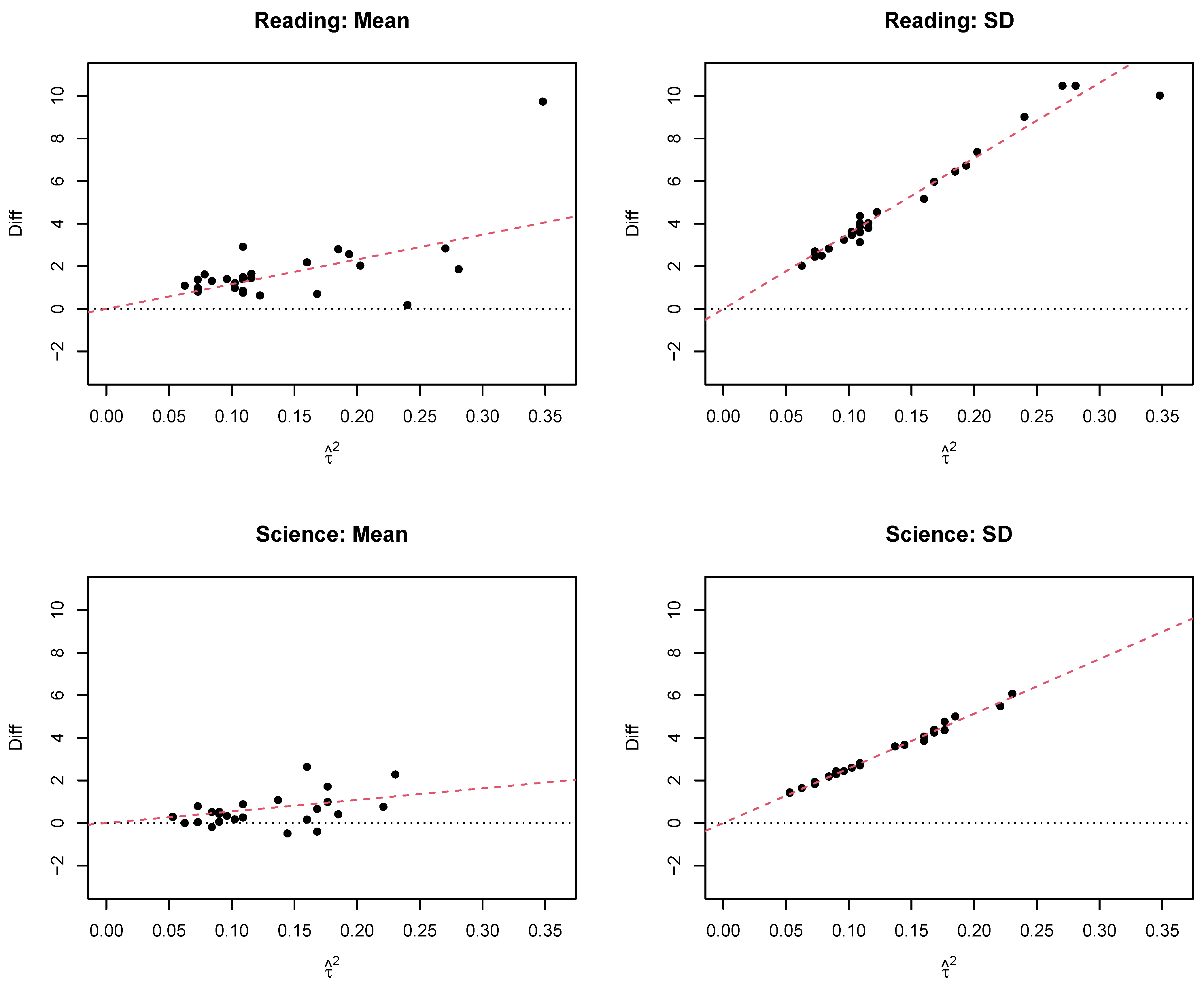
4.2.2. Reading
4.2.3. Science
4.2.4. Summary
5. Discussion
Funding
Institutional Review Board Statement
Informed Consent Statement
Data Availability Statement
Conflicts of Interest
Abbreviations
| 2PL | two-parameter logistic |
| BCFIPC | bias-corrected fixed item parameter calibration |
| DIF | differential item functioning |
| FIPC | fixed item parameter calibration |
| IRF | item response function |
| IRT | item response theory |
| LSA | large-scale assessment |
| MGM | mean-geometric mean |
| MML | marginal maximum likelihood |
| PISA | programme for international student assessment |
| RMSE | root mean square error |
| SD | standard deviation |
| SIMEX | simulation extrapolation |
Appendix A. Additional Results for the Simulation Study

| FIPC for | BCFIPC for | |||||||||||||
|---|---|---|---|---|---|---|---|---|---|---|---|---|---|---|
| 0 | −0.3 | 15 | 0.001 | 0.000 | −0.001 | 0.000 | 0.000 | 0.000 | 0.000 | 0.000 | −0.001 | 0.000 | 0.000 | 0.000 |
| 30 | −0.001 | 0.001 | 0.001 | 0.000 | 0.000 | 0.000 | −0.001 | 0.001 | 0.000 | 0.000 | 0.000 | 0.000 | ||
| 45 | 0.001 | 0.002 | 0.001 | 0.000 | 0.001 | 0.000 | 0.001 | 0.002 | 0.001 | 0.000 | 0.001 | 0.000 | ||
| 0 | 15 | 0.000 | −0.002 | −0.001 | 0.000 | −0.001 | 0.000 | 0.000 | −0.002 | −0.001 | 0.000 | −0.001 | 0.000 | |
| 30 | 0.001 | 0.000 | 0.000 | 0.000 | 0.000 | 0.000 | 0.001 | 0.000 | 0.000 | 0.000 | 0.000 | 0.000 | ||
| 45 | −0.001 | 0.000 | −0.001 | 0.001 | 0.000 | 0.000 | −0.002 | 0.000 | −0.001 | 0.001 | 0.000 | 0.000 | ||
| 0.3 | 15 | 0.002 | 0.000 | 0.000 | −0.001 | 0.000 | 0.000 | 0.002 | 0.000 | 0.000 | −0.001 | 0.000 | 0.000 | |
| 30 | 0.000 | −0.002 | −0.001 | 0.000 | 0.000 | 0.000 | 0.000 | −0.002 | −0.001 | 0.000 | 0.000 | 0.000 | ||
| 45 | 0.000 | 0.001 | −0.002 | 0.000 | 0.000 | 0.000 | 0.000 | 0.001 | −0.002 | 0.000 | 0.000 | 0.000 | ||
| 0.6 | 15 | 0.002 | −0.001 | 0.000 | 0.000 | 0.001 | 0.000 | 0.002 | −0.001 | 0.001 | 0.000 | 0.001 | 0.000 | |
| 30 | 0.001 | −0.001 | 0.001 | 0.000 | 0.000 | 0.000 | 0.001 | −0.001 | 0.001 | 0.000 | 0.000 | 0.000 | ||
| 45 | 0.001 | −0.002 | −0.001 | 0.001 | 0.000 | 0.000 | 0.001 | −0.002 | 0.000 | 0.001 | 0.000 | 0.000 | ||
| 0.2 | −0.3 | 15 | 0.005 | 0.005 | 0.004 | 0.003 | 0.003 | 0.003 | 0.002 | 0.001 | 0.000 | −0.001 | −0.001 | −0.001 |
| 30 | 0.005 | 0.004 | 0.004 | 0.005 | 0.004 | 0.005 | 0.001 | 0.001 | 0.000 | 0.001 | 0.000 | 0.001 | ||
| 45 | 0.001 | 0.004 | 0.006 | 0.004 | 0.005 | 0.004 | −0.002 | 0.000 | 0.002 | 0.000 | 0.001 | 0.000 | ||
| 0 | 15 | 0.004 | 0.004 | 0.001 | 0.002 | 0.001 | 0.003 | 0.002 | 0.003 | −0.001 | 0.001 | −0.001 | 0.001 | |
| 30 | −0.002 | 0.000 | 0.001 | 0.003 | 0.001 | 0.001 | −0.004 | −0.001 | −0.001 | 0.001 | 0.000 | 0.000 | ||
| 45 | 0.000 | 0.002 | 0.004 | 0.002 | 0.001 | 0.002 | −0.001 | 0.000 | 0.002 | 0.001 | −0.001 | 0.000 | ||
| 0.3 | 15 | 0.003 | −0.003 | −0.001 | 0.001 | 0.000 | −0.001 | 0.004 | −0.002 | 0.000 | 0.002 | 0.000 | 0.000 | |
| 30 | −0.001 | 0.001 | 0.000 | 0.001 | −0.002 | 0.000 | 0.000 | 0.001 | 0.000 | 0.002 | −0.001 | 0.001 | ||
| 45 | 0.001 | −0.002 | −0.001 | 0.001 | −0.001 | −0.001 | 0.001 | −0.002 | −0.001 | 0.001 | 0.000 | 0.000 | ||
| 0.6 | 15 | −0.002 | −0.003 | −0.003 | −0.004 | −0.002 | −0.003 | 0.001 | 0.000 | 0.000 | −0.001 | 0.001 | 0.000 | |
| 30 | −0.005 | −0.003 | −0.005 | −0.005 | −0.003 | −0.003 | −0.002 | −0.001 | −0.002 | −0.002 | 0.000 | 0.000 | ||
| 45 | −0.004 | −0.002 | −0.004 | −0.002 | −0.003 | −0.003 | −0.002 | 0.001 | −0.001 | 0.001 | 0.000 | −0.001 | ||
| 0.4 | −0.3 | 15 | 0.016 | 0.014 | 0.016 | 0.017 | 0.016 | 0.017 | 0.002 | −0.001 | 0.000 | 0.002 | 0.001 | 0.002 |
| 30 | 0.015 | 0.015 | 0.016 | 0.015 | 0.015 | 0.014 | 0.000 | 0.000 | 0.001 | 0.000 | −0.001 | −0.002 | ||
| 45 | 0.015 | 0.014 | 0.013 | 0.012 | 0.014 | 0.014 | 0.000 | −0.001 | −0.002 | −0.004 | −0.001 | −0.001 | ||
| 0 | 15 | 0.005 | 0.009 | 0.008 | 0.005 | 0.005 | 0.004 | −0.002 | 0.002 | 0.001 | −0.002 | −0.002 | −0.003 | |
| 30 | 0.009 | 0.008 | 0.007 | 0.010 | 0.007 | 0.009 | 0.002 | 0.002 | 0.000 | 0.003 | 0.000 | 0.002 | ||
| 45 | 0.006 | 0.007 | 0.009 | 0.008 | 0.006 | 0.007 | −0.001 | 0.001 | 0.002 | 0.001 | −0.001 | 0.000 | ||
| 0.3 | 15 | 0.000 | −0.004 | 0.000 | −0.002 | −0.001 | −0.003 | 0.002 | −0.002 | 0.002 | 0.000 | 0.001 | −0.001 | |
| 30 | −0.001 | −0.005 | −0.002 | −0.005 | 0.000 | −0.001 | 0.001 | −0.003 | 0.000 | −0.003 | 0.002 | 0.001 | ||
| 45 | −0.003 | −0.003 | −0.003 | −0.002 | 0.000 | 0.001 | −0.001 | −0.001 | −0.001 | 0.000 | 0.002 | 0.003 | ||
| 0.6 | 15 | −0.014 | −0.010 | −0.014 | −0.009 | −0.010 | −0.014 | −0.003 | 0.002 | −0.003 | 0.003 | 0.001 | −0.003 | |
| 30 | −0.012 | −0.010 | −0.011 | −0.009 | −0.013 | −0.010 | −0.001 | 0.001 | 0.000 | 0.002 | −0.002 | 0.001 | ||
| 45 | −0.009 | −0.012 | −0.011 | −0.011 | −0.011 | −0.009 | 0.002 | −0.001 | 0.000 | 0.000 | 0.000 | 0.002 | ||
| FIPC for | BCFIPC for | |||||||||||||
|---|---|---|---|---|---|---|---|---|---|---|---|---|---|---|
| 0 | −0.3 | 15 | −0.006 | −0.004 | −0.002 | 0.000 | −0.001 | 0.000 | −0.004 | −0.004 | −0.001 | 0.000 | −0.001 | 0.000 |
| 30 | −0.003 | −0.002 | −0.001 | 0.000 | −0.001 | 0.000 | −0.002 | −0.002 | −0.001 | 0.000 | −0.001 | 0.000 | ||
| 45 | −0.006 | −0.004 | −0.002 | −0.001 | 0.000 | 0.000 | −0.005 | −0.003 | −0.001 | −0.001 | 0.000 | 0.000 | ||
| 0 | 15 | −0.005 | −0.004 | −0.003 | 0.000 | −0.001 | 0.000 | −0.004 | −0.003 | −0.002 | 0.000 | −0.001 | 0.000 | |
| 30 | −0.004 | −0.003 | 0.000 | −0.001 | 0.000 | 0.000 | −0.003 | −0.002 | 0.000 | −0.001 | 0.000 | 0.000 | ||
| 45 | −0.006 | −0.002 | 0.000 | −0.001 | −0.001 | 0.000 | −0.005 | −0.001 | 0.000 | −0.001 | 0.000 | 0.000 | ||
| 0.3 | 15 | −0.006 | −0.004 | 0.000 | 0.000 | 0.000 | 0.000 | −0.004 | −0.003 | 0.000 | 0.000 | 0.000 | 0.000 | |
| 30 | −0.005 | −0.003 | 0.000 | 0.000 | 0.000 | 0.000 | −0.004 | −0.002 | 0.000 | 0.000 | 0.000 | 0.000 | ||
| 45 | −0.005 | −0.002 | 0.000 | −0.001 | −0.001 | 0.000 | −0.004 | −0.002 | 0.000 | −0.001 | 0.000 | 0.000 | ||
| 0.6 | 15 | −0.004 | −0.003 | −0.002 | 0.000 | −0.001 | 0.000 | −0.002 | −0.002 | −0.001 | 0.000 | 0.000 | 0.000 | |
| 30 | −0.006 | −0.002 | −0.002 | −0.001 | 0.000 | 0.000 | −0.005 | −0.002 | −0.001 | −0.001 | 0.000 | 0.000 | ||
| 45 | −0.006 | −0.004 | −0.001 | 0.000 | 0.000 | 0.000 | −0.005 | −0.004 | −0.001 | 0.000 | 0.000 | 0.000 | ||
| 0.2 | −0.3 | 15 | −0.011 | −0.011 | −0.007 | −0.007 | −0.008 | −0.007 | −0.004 | −0.003 | 0.001 | 0.002 | 0.001 | 0.002 |
| 30 | −0.011 | −0.010 | −0.008 | −0.007 | −0.007 | −0.006 | −0.004 | −0.004 | −0.001 | 0.000 | 0.001 | 0.001 | ||
| 45 | −0.010 | −0.009 | −0.007 | −0.006 | −0.006 | −0.006 | −0.004 | −0.003 | 0.000 | 0.001 | 0.000 | 0.000 | ||
| 0 | 15 | −0.016 | −0.011 | −0.009 | −0.009 | −0.008 | −0.008 | −0.008 | −0.003 | 0.000 | 0.000 | 0.002 | 0.002 | |
| 30 | −0.011 | −0.008 | −0.009 | −0.008 | −0.007 | −0.007 | −0.005 | −0.001 | −0.002 | 0.000 | 0.001 | 0.001 | ||
| 45 | −0.013 | −0.008 | −0.009 | −0.007 | −0.007 | −0.006 | −0.007 | −0.001 | −0.002 | 0.000 | 0.000 | 0.001 | ||
| 0.3 | 15 | −0.016 | −0.012 | −0.009 | −0.008 | −0.008 | −0.008 | −0.007 | −0.003 | 0.000 | 0.001 | 0.001 | 0.002 | |
| 30 | −0.013 | −0.009 | −0.009 | −0.008 | −0.007 | −0.007 | −0.006 | −0.002 | −0.001 | 0.000 | 0.001 | 0.001 | ||
| 45 | −0.013 | −0.009 | −0.008 | −0.007 | −0.007 | −0.007 | −0.007 | −0.002 | −0.001 | 0.001 | 0.000 | 0.001 | ||
| 0.6 | 15 | −0.016 | −0.011 | −0.009 | −0.009 | −0.007 | −0.008 | −0.007 | −0.001 | 0.001 | 0.001 | 0.003 | 0.003 | |
| 30 | −0.013 | −0.010 | −0.009 | −0.008 | −0.009 | −0.007 | −0.005 | −0.002 | −0.001 | 0.000 | 0.000 | 0.001 | ||
| 45 | −0.013 | −0.008 | −0.008 | −0.008 | −0.007 | −0.007 | −0.006 | −0.001 | −0.001 | 0.000 | 0.000 | 0.001 | ||
| 0.4 | −0.3 | 15 | −0.031 | −0.030 | −0.029 | −0.027 | −0.027 | −0.028 | 0.003 | 0.006 | 0.006 | 0.008 | 0.009 | 0.008 |
| 30 | −0.029 | −0.027 | −0.025 | −0.025 | −0.025 | −0.024 | −0.001 | 0.002 | 0.004 | 0.004 | 0.004 | 0.004 | ||
| 45 | −0.030 | −0.027 | −0.024 | −0.023 | −0.023 | −0.023 | −0.004 | −0.001 | 0.002 | 0.003 | 0.003 | 0.003 | ||
| 0 | 15 | −0.037 | −0.033 | −0.030 | −0.030 | −0.029 | −0.030 | 0.000 | 0.005 | 0.008 | 0.009 | 0.009 | 0.009 | |
| 30 | −0.030 | −0.027 | −0.027 | −0.027 | −0.027 | −0.026 | 0.000 | 0.003 | 0.004 | 0.004 | 0.004 | 0.005 | ||
| 45 | −0.030 | −0.027 | −0.026 | −0.027 | −0.025 | −0.025 | −0.002 | 0.001 | 0.002 | 0.002 | 0.004 | 0.004 | ||
| 0.3 | 15 | −0.038 | −0.033 | −0.031 | −0.030 | −0.031 | −0.031 | 0.001 | 0.005 | 0.008 | 0.009 | 0.009 | 0.009 | |
| 30 | −0.034 | −0.028 | −0.028 | −0.028 | −0.027 | −0.027 | −0.003 | 0.004 | 0.004 | 0.004 | 0.005 | 0.005 | ||
| 45 | −0.032 | −0.029 | −0.027 | −0.027 | −0.026 | −0.027 | −0.003 | 0.000 | 0.002 | 0.002 | 0.004 | 0.003 | ||
| 0.6 | 15 | −0.037 | −0.034 | −0.034 | −0.029 | −0.030 | −0.031 | 0.003 | 0.006 | 0.007 | 0.011 | 0.010 | 0.009 | |
| 30 | −0.035 | −0.030 | −0.029 | −0.028 | −0.028 | −0.028 | −0.003 | 0.002 | 0.003 | 0.004 | 0.005 | 0.005 | ||
| 45 | −0.029 | −0.030 | −0.027 | −0.027 | −0.027 | −0.026 | 0.000 | 0.000 | 0.003 | 0.003 | 0.003 | 0.004 | ||
| for | for | |||||||||||||
|---|---|---|---|---|---|---|---|---|---|---|---|---|---|---|
| 0 | −0.3 | 15 | 100.1 | 100.1 | 100.1 | 100.0 | 100.0 | 100.0 | 100.1 | 99.8 | 100.0 | 100.0 | 100.0 | 100.0 |
| 30 | 100.1 | 100.1 | 100.0 | 100.0 | 100.0 | 100.0 | 99.9 | 100.0 | 100.0 | 100.0 | 100.0 | 100.0 | ||
| 45 | 100.0 | 100.0 | 100.0 | 100.0 | 100.0 | 100.0 | 99.9 | 99.9 | 100.0 | 100.0 | 100.0 | 100.0 | ||
| 0 | 15 | 100.1 | 100.1 | 100.0 | 100.0 | 100.0 | 100.0 | 99.9 | 99.9 | 100.0 | 100.1 | 100.0 | 100.0 | |
| 30 | 100.1 | 100.0 | 100.0 | 100.0 | 100.0 | 100.0 | 100.0 | 100.0 | 100.0 | 100.0 | 100.0 | 100.0 | ||
| 45 | 100.1 | 100.0 | 100.0 | 100.0 | 100.0 | 100.0 | 99.9 | 99.9 | 100.0 | 100.0 | 100.0 | 100.0 | ||
| 0.3 | 15 | 100.1 | 100.1 | 100.0 | 100.0 | 100.0 | 100.0 | 100.0 | 99.9 | 100.0 | 100.0 | 100.0 | 100.0 | |
| 30 | 100.1 | 100.0 | 100.0 | 100.0 | 100.0 | 100.0 | 100.0 | 100.0 | 100.0 | 100.0 | 100.0 | 100.0 | ||
| 45 | 100.1 | 100.0 | 100.0 | 100.0 | 100.0 | 100.0 | 99.9 | 100.0 | 100.0 | 100.0 | 100.0 | 100.0 | ||
| 0.6 | 15 | 100.2 | 100.1 | 100.0 | 100.0 | 100.0 | 100.0 | 99.9 | 99.9 | 99.9 | 100.0 | 100.0 | 100.0 | |
| 30 | 100.2 | 100.1 | 100.0 | 100.0 | 100.0 | 100.0 | 99.9 | 100.0 | 100.0 | 100.0 | 100.0 | 100.0 | ||
| 45 | 100.1 | 100.0 | 100.0 | 100.0 | 100.0 | 100.0 | 99.9 | 99.9 | 99.9 | 100.0 | 100.0 | 100.0 | ||
| 0.2 | −0.3 | 15 | 100.6 | 100.5 | 100.4 | 100.5 | 100.5 | 100.6 | 99.6 | 98.9 | 99.2 | 98.7 | 97.0 | 96.6 |
| 30 | 100.5 | 100.4 | 100.5 | 100.2 | 100.3 | 100.0 | 99.3 | 98.4 | 97.9 | 97.1 | 95.5 | 94.9 | ||
| 45 | 100.7 | 100.4 | 100.0 | 100.2 | 99.9 | 100.2 | 99.1 | 98.7 | 98.2 | 97.5 | 95.2 | 92.5 | ||
| 0 | 15 | 100.6 | 100.6 | 100.8 | 100.7 | 100.7 | 100.6 | 98.9 | 98.6 | 98.5 | 97.4 | 97.2 | 95.5 | |
| 30 | 100.7 | 100.7 | 100.7 | 100.6 | 100.7 | 100.7 | 99.0 | 98.9 | 97.5 | 96.2 | 94.6 | 93.2 | ||
| 45 | 100.7 | 100.6 | 100.5 | 100.6 | 100.7 | 100.6 | 98.9 | 99.0 | 96.8 | 96.0 | 93.8 | 92.0 | ||
| 0.3 | 15 | 100.8 | 100.7 | 100.8 | 100.8 | 100.8 | 100.8 | 99.1 | 98.5 | 98.7 | 97.5 | 95.9 | 96.6 | |
| 30 | 100.7 | 100.7 | 100.7 | 100.8 | 100.7 | 100.8 | 98.8 | 98.8 | 97.6 | 95.6 | 94.6 | 91.8 | ||
| 45 | 100.7 | 100.7 | 100.7 | 100.8 | 100.8 | 100.8 | 98.6 | 98.5 | 97.3 | 96.6 | 92.7 | 90.1 | ||
| 0.6 | 15 | 100.7 | 100.7 | 100.7 | 100.7 | 100.8 | 100.6 | 98.9 | 98.8 | 98.0 | 97.4 | 98.3 | 96.1 | |
| 30 | 100.7 | 100.7 | 100.5 | 100.4 | 100.7 | 100.5 | 99.4 | 98.8 | 97.3 | 96.1 | 92.9 | 92.0 | ||
| 45 | 100.6 | 100.7 | 100.5 | 100.7 | 100.5 | 100.4 | 98.7 | 98.9 | 97.5 | 95.4 | 92.9 | 90.8 | ||
| 0.4 | −0.3 | 15 | 101.8 | 102.0 | 101.9 | 101.6 | 101.6 | 101.6 | 95.6 | 93.6 | 90.5 | 89.6 | 88.7 | 86.8 |
| 30 | 101.8 | 101.2 | 101.0 | 100.9 | 100.9 | 101.2 | 94.1 | 91.2 | 86.9 | 82.2 | 78.2 | 77.0 | ||
| 45 | 101.7 | 101.3 | 101.2 | 101.3 | 100.4 | 100.5 | 92.2 | 88.1 | 84.3 | 78.9 | 74.7 | 69.6 | ||
| 0 | 15 | 102.8 | 102.8 | 102.9 | 103.0 | 102.9 | 103.0 | 93.2 | 92.0 | 90.7 | 88.1 | 86.2 | 83.9 | |
| 30 | 102.7 | 102.6 | 102.6 | 102.4 | 102.7 | 102.5 | 93.1 | 91.0 | 85.0 | 79.2 | 74.3 | 73.3 | ||
| 45 | 102.7 | 102.6 | 102.3 | 102.3 | 102.6 | 102.5 | 91.5 | 87.3 | 82.3 | 73.5 | 71.8 | 68.1 | ||
| 0.3 | 15 | 103.2 | 103.1 | 103.2 | 103.2 | 103.2 | 103.3 | 93.3 | 91.3 | 88.7 | 87.8 | 84.6 | 82.0 | |
| 30 | 103.2 | 103.1 | 103.1 | 103.1 | 103.2 | 103.1 | 91.3 | 90.1 | 83.2 | 77.8 | 74.1 | 72.5 | ||
| 45 | 103.1 | 103.1 | 103.1 | 103.1 | 103.2 | 103.3 | 90.7 | 86.1 | 79.8 | 72.5 | 68.4 | 63.1 | ||
| 0.6 | 15 | 102.7 | 103.2 | 102.8 | 103.3 | 102.9 | 102.3 | 93.3 | 91.6 | 87.5 | 88.1 | 84.8 | 82.2 | |
| 30 | 102.6 | 102.8 | 102.4 | 102.6 | 101.7 | 102.4 | 90.6 | 88.2 | 82.4 | 77.0 | 74.2 | 70.0 | ||
| 45 | 102.8 | 102.1 | 102.0 | 101.9 | 101.8 | 102.3 | 92.5 | 85.3 | 80.4 | 73.4 | 67.9 | 64.8 | ||
Appendix B. Country Labels for PISA 2006 Mathematics Study
References
- Bock, R.D.; Moustaki, I. Item response theory in a general framework. In Handbook of Statistics, Vol. 26: Psychometrics; Rao, C.R., Sinharay, S., Eds.; Elsevier: Amsterdam, The Netherlands, 2007; pp. 469–513. [Google Scholar] [CrossRef]
- Bock, R.D.; Gibbons, R.D. Item Response Theory; Wiley: New York, NY, USA, 2021. [Google Scholar] [CrossRef]
- Chen, Y.; Li, X.; Liu, J.; Ying, Z. Item response theory—A statistical framework for educational and psychological measurement. Stat. Sci. 2024; epub ahead of print. Available online: https://rb.gy/1yic0e (accessed on 19 March 2025).
- Sijtsma, K.; van der Ark, L.A. Measurement Models for Psychological Attributes; CRC Press: Boca Raton, FL, USA, 2020. [Google Scholar] [CrossRef]
- van der Linden, W.J. Unidimensional logistic response models. In Handbook of Item Response Theory, Volume 1: Models; van der Linden, W.J., Ed.; CRC Press: Boca Raton, FL, USA, 2016; pp. 11–30. [Google Scholar] [CrossRef]
- Yen, W.M.; Fitzpatrick, A.R. Item response theory. In Educational Measurement; Brennan, R.L., Ed.; Praeger Publishers: Westport, CT, USA, 2006; pp. 111–154. [Google Scholar]
- Birnbaum, A. Some latent trait models and their use in inferring an examinee’s ability. In Statistical Theories of Mental Test Scores; Lord, F.M., Novick, M.R., Eds.; MIT Press: Reading, MA, USA, 1968; pp. 397–479. [Google Scholar]
- Aitkin, M. Expectation maximization algorithm and extensions. In Handbook of Item Response Theory, Volume 2: Statistical Tools; van der Linden, W.J., Ed.; CRC Press: Boca Raton, FL, USA, 2016; pp. 217–236. [Google Scholar] [CrossRef]
- Bock, R.D.; Aitkin, M. Marginal maximum likelihood estimation of item parameters: Application of an EM algorithm. Psychometrika 1981, 46, 443–459. [Google Scholar] [CrossRef]
- Glas, C.A.W. Maximum-likelihood estimation. In Handbook of Item Response Theory, Volume 2: Statistical Tools; van der Linden, W.J., Ed.; CRC Press: Boca Raton, FL, USA, 2016; pp. 197–216. [Google Scholar] [CrossRef]
- Lietz, P.; Cresswell, J.C.; Rust, K.F.; Adams, R.J. (Eds.) Implementation of Large-Scale Education Assessments; Wiley: New York, NY, USA, 2017. [Google Scholar] [CrossRef]
- Rutkowski, L.; von Davier, M.; Rutkowski, D. (Eds.) A Handbook of International Large-Scale Assessment: Background, Technical Issues, and Methods of Data Analysis; Chapman Hall/CRC Press: London, UK, 2013. [Google Scholar] [CrossRef]
- OECD. PISA 2006. Technical Report; OECD: Paris, France, 2009; Available online: https://bit.ly/3xfxdwD (accessed on 19 March 2025).
- Kim, S. A comparative study of IRT fixed parameter calibration methods. J. Educ. Meas. 2006, 43, 355–381. [Google Scholar] [CrossRef]
- König, C.; Khorramdel, L.; Yamamoto, K.; Frey, A. The benefits of fixed item parameter calibration for parameter accuracy in small sample situations in large-scale assessments. Educ. Meas. 2021, 40, 17–27. [Google Scholar] [CrossRef]
- Mellenbergh, G.J. Item bias and item response theory. Int. J. Educ. Res. 1989, 13, 127–143. [Google Scholar] [CrossRef]
- Meredith, W. Measurement invariance, factor analysis and factorial invariance. Psychometrika 1993, 58, 525–543. [Google Scholar] [CrossRef]
- Millsap, R.E. Statistical Approaches to Measurement Invariance; Routledge: New York, NY, USA, 2011. [Google Scholar] [CrossRef]
- Penfield, R.D.; Camilli, G. Differential item functioning and item bias. In Handbook of Statistics, Vol. 26: Psychometrics; Rao, C.R., Sinharay, S., Eds.; Elsevier: Amsterdam, The Netherlands, 2007; pp. 125–167. [Google Scholar] [CrossRef]
- Michaelides, M.P. A review of the effects on IRT item parameter estimates with a focus on misbehaving common items in test equating. Front. Psychol. 2010, 1, 167. [Google Scholar] [CrossRef] [PubMed]
- Michaelides, M.P.; Haertel, E.H. Selection of common items as an unrecognized source of variability in test equating: A bootstrap approximation assuming random sampling of common items. Appl. Meas. Educ. 2014, 27, 46–57. [Google Scholar] [CrossRef]
- Monseur, C.; Berezner, A. The computation of equating errors in international surveys in education. J. Appl. Meas. 2007, 8, 323–335. Available online: https://bit.ly/2WDPeqD (accessed on 19 March 2025).
- Monseur, C.; Sibberns, H.; Hastedt, D. Linking errors in trend estimation for international surveys in education. IERI Monogr. Ser. 2008, 1, 113–122. [Google Scholar]
- Robitzsch, A. Linking error in the 2PL model. J 2023, 6, 58–84. [Google Scholar] [CrossRef]
- Robitzsch, A. Estimation of standard error, linking error, and total error for robust and nonrobust linking methods in the two-parameter logistic model. Stats 2024, 7, 592–612. [Google Scholar] [CrossRef]
- Sachse, K.A.; Roppelt, A.; Haag, N. A comparison of linking methods for estimating national trends in international comparative large-scale assessments in the presence of cross-national DIF. J. Educ. Meas. 2016, 53, 152–171. [Google Scholar] [CrossRef]
- Sachse, K.A.; Haag, N. Standard errors for national trends in international large-scale assessments in the case of cross-national differential item functioning. Appl. Meas. Educ. 2017, 30, 102–116. [Google Scholar] [CrossRef]
- Wu, M. Measurement, sampling, and equating errors in large-scale assessments. Educ. Meas. 2010, 29, 15–27. [Google Scholar] [CrossRef]
- De Boeck, P. Random item IRT models. Psychometrika 2008, 73, 533–559. [Google Scholar] [CrossRef]
- Fox, J.P.; Verhagen, A.J. Random item effects modeling for cross-national survey data. In Cross-Cultural Analysis: Methods and Applications; Davidov, E., Schmidt, P., Billiet, J., Eds.; Routledge: London, UK, 2010; pp. 461–482. [Google Scholar] [CrossRef]
- de Jong, M.G.; Steenkamp, J.B.E.M.; Fox, J.P. Relaxing measurement invariance in cross-national consumer research using a hierarchical IRT model. J. Consum. Res. 2007, 34, 260–278. [Google Scholar] [CrossRef]
- Robitzsch, A. Analytical approximation of the jackknife linking error in item response models utilizing a Taylor expansion of the log-likelihood function. AppliedMath 2023, 3, 49–59. [Google Scholar] [CrossRef]
- Robitzsch, A. Bias and linking error in fixed item parameter calibration. AppliedMath 2024, 4, 1181–1191. [Google Scholar] [CrossRef]
- Robitzsch, A. Linking error estimation in fixed item parameter calibration: Theory and application in large-scale assessment studies. Foundations 2025, 5, 4. [Google Scholar] [CrossRef]
- Glas, C.A.W.; Jehangir, M. Modeling country-specific differential functioning. In A Handbook of International Large-Scale Assessment: Background, Technical Issues, and Methods of Data Analysis; Rutkowski, L., von Davier, M., Rutkowski, D., Eds.; Chapman Hall/CRC Press: London, UK, 2013; pp. 97–115. [Google Scholar] [CrossRef]
- von Davier, M.; Yamamoto, K.; Shin, H.J.; Chen, H.; Khorramdel, L.; Weeks, J.; Davis, S.; Kong, N.; Kandathil, M. Evaluating item response theory linking and model fit for data from PISA 2000–2012. Assess. Educ. 2019, 26, 466–488. [Google Scholar] [CrossRef]
- Yuan, K.H.; Cheng, Y.; Patton, J. Information matrices and standard errors for MLEs of item parameters in IRT. Psychometrika 2014, 79, 232–254. [Google Scholar] [CrossRef]
- Boos, D.D.; Stefanski, L.A. Essential Statistical Inference; Springer: New York, NY, USA, 2013. [Google Scholar] [CrossRef]
- White, H. Maximum likelihood estimation of misspecified models. Econometrica 1982, 50, 1–25. [Google Scholar] [CrossRef]
- Frey, A.; Hartig, J.; Rupp, A.A. An NCME instructional module on booklet designs in large-scale assessments of student achievement: Theory and practice. Educ. Meas. 2009, 28, 39–53. [Google Scholar] [CrossRef]
- Pokropek, A. Missing by design: Planned missing-data designs in social science. ASK Res. Meth. 2011, 20, 81–105. Available online: https://tinyurl.com/3px352sy (accessed on 19 March 2025).
- R Core Team. R: A Language and Environment for Statistical Computing; R Foundation for Statistical Computing: Vienna, Austria, 2024; Available online: https://www.R-project.org (accessed on 15 June 2024).
- Robitzsch, A. sirt: Supplementary Item Response Theory Models. R Package Version 4.2-106. 2024. Available online: https://github.com/alexanderrobitzsch/sirt (accessed on 31 December 2024).
- Kolenikov, S. Resampling variance estimation for complex survey data. Stata J. 2010, 10, 165–199. [Google Scholar] [CrossRef]
- Särndal, C.E.; Swensson, B.; Wretman, J. Model Assisted Survey Sampling; Springer: New York, NY, USA, 1992. [Google Scholar] [CrossRef]
- OECD. PISA 2018. Technical Report; OECD: Paris, France, 2020; Available online: https://bit.ly/3zWbidA (accessed on 19 March 2025).
- Boer, D.; Hanke, K.; He, J. On detecting systematic measurement error in cross-cultural research: A review and critical reflection on equivalence and invariance tests. J. Cross-Cult. Psychol. 2018, 49, 713–734. [Google Scholar] [CrossRef]
- He, J.; Barrera-Pedemonte, F.; Buchholz, J. Cross-cultural comparability of noncognitive constructs in TIMSS and PISA. Assess. Educ. 2019, 26, 369–385. [Google Scholar] [CrossRef]
- Kankaraš, M.; Moors, G. Analysis of cross-cultural comparability of PISA 2009 scores. J. Cross-Cult. Psychol. 2014, 45, 381–399. [Google Scholar] [CrossRef]
- Rutkowski, L.; Svetina, D. Assessing the hypothesis of measurement invariance in the context of large-scale international surveys. Educ. Psychol. Meas. 2014, 74, 31–57. [Google Scholar] [CrossRef]
- Stefanski, L.A.; Boos, D.D. The calculus of M-estimation. Am. Stat. 2002, 56, 29–38. [Google Scholar] [CrossRef]
- Lohr, S.L. Sampling: Design and Analysis; Chapman and Hall/CRC: Boca Raton, FL, USA, 2021. [Google Scholar] [CrossRef]
- Lumley, T. Complex Surveys: A Guide to Analysis Using R; John Wiley & Sons: New York, NY, USA, 2011. [Google Scholar] [CrossRef]
- Rasch, G. Probabilistic Models for Some Intelligence and Attainment Tests; Danish Institute for Educational Research: Copenhagen, Denmark, 1960. [Google Scholar]
- Bond, T.; Yan, Z.; Heene, M. Applying the Rasch Model; Routledge: New York, NY, USA, 2020. [Google Scholar] [CrossRef]
- Debelak, R.; Strobl, C.; Zeigenfuse, M.D. An Introduction to the Rasch Model with Examples in R; CRC Press: Boca Raton, FL, USA, 2022. [Google Scholar] [CrossRef]
- Engelhard, G. Invariant Measurement; Routledge: New York, NY, USA, 2012. [Google Scholar] [CrossRef]
- De Ayala, R.J. The Theory and Practice of Item Response Theory; Guilford Publications: New York, NY, USA, 2022. [Google Scholar]
- Lord, F.M. Applications of Item Response Theory to Practical Testing Problems; Erlbaum: Hillsdale, NJ, USA, 1980. [Google Scholar] [CrossRef]
- Culpepper, S.A. The prevalence and implications of slipping on low-stakes, large-scale assessments. J. Educ. Behav. Stat. 2017, 42, 706–725. [Google Scholar] [CrossRef]
- Falk, C.F.; Cai, L. Semiparametric item response functions in the context of guessing. J. Educ. Meas. 2016, 53, 229–247. [Google Scholar] [CrossRef]
- Feuerstahler, L. Flexible item response modeling in R with the flexmet package. Psych 2021, 3, 447–478. [Google Scholar] [CrossRef]
- Lee, S.; Bolt, D.M. An alternative to the 3PL: Using asymmetric item characteristic curves to address guessing effects. J. Educ. Meas. 2018, 55, 90–111. [Google Scholar] [CrossRef]
- Liao, X.; Bolt, D.M. Item characteristic curve asymmetry: A better way to accommodate slips and guesses than a four-parameter model? J. Educ. Behav. Stat. 2021, 46, 753–775. [Google Scholar] [CrossRef]
- Carroll, R.J.; Küchenhoff, H.; Lombard, F.; Stefanski, L.A. Asymptotics for the SIMEX estimator in nonlinear measurement error models. J. Am. Stat. Assoc. 1996, 91, 242–250. [Google Scholar] [CrossRef]
- Carroll, R.J.; Ruppert, D.; Stefanski, L.A.; Crainiceanu, C.M. Measurement Error in Nonlinear Models; CRC Press: Boca Raton, FL, USA, 2006. [Google Scholar] [CrossRef]
- Cook, J.R.; Stefanski, L.A. Simulation-extrapolation estimation in parametric measurement error models. J. Am. Stat. Assoc. 1994, 89, 1314–1328. [Google Scholar] [CrossRef]
- Robitzsch, A. SIMEX-based and analytical bias corrections in Stocking-Lord linking. Analytics 2024, 3, 368–388. [Google Scholar] [CrossRef]
- Robitzsch, A. Implementation aspects in simulation extrapolation-based Stocking–Lord linking. Appl. Sci. 2025, 15, 901. [Google Scholar] [CrossRef]
- Levy, R. The rise of Markov chain Monte Carlo estimation for psychometric modeling. J. Probab. Stat. 2009, 2009, 537139. [Google Scholar] [CrossRef]
- Levy, R.; Mislevy, R.J.; Sinharay, S. Posterior predictive model checking for multidimensionality in item response theory. Appl. Psychol. Meas. 2009, 33, 519–537. [Google Scholar] [CrossRef]
- Haberman, S.J.; Sinharay, S.; Chon, K.H. Assessing item fit for unidimensional item response theory models using residuals from estimated item response functions. Psychometrika 2013, 78, 417–440. [Google Scholar] [CrossRef]
- van Rijn, P.W.; Sinharay, S.; Haberman, S.J.; Johnson, M.S. Assessment of fit of item response theory models used in large-scale educational survey assessments. Large-Scale Assess. Educ. 2016, 4, 10. [Google Scholar] [CrossRef]
- Robitzsch, A.; Lüdtke, O. Some thoughts on analytical choices in the scaling model for test scores in international large-scale assessment studies. Meas. Instrum. Soc. Sci. 2022, 4, 9. [Google Scholar] [CrossRef]
- Brennan, R.L. Misconceptions at the intersection of measurement theory and practice. Educ. Meas. 1998, 17, 5–9. [Google Scholar] [CrossRef]
- Camilli, G. IRT scoring and test blueprint fidelity. Appl. Psychol. Meas. 2018, 42, 393–400. [Google Scholar] [CrossRef]
- Chiu, T.W.; Camilli, G. Comment on 3PL IRT adjustment for guessing. Appl. Psychol. Meas. 2013, 37, 76–86. [Google Scholar] [CrossRef]
- Haebara, T. Equating logistic ability scales by a weighted least squares method. Jpn. Psychol. Res. 1980, 22, 144–149. [Google Scholar] [CrossRef]
- Stocking, M.L.; Lord, F.M. Developing a common metric in item response theory. Appl. Psychol. Meas. 1983, 7, 201–210. [Google Scholar] [CrossRef]
- Robitzsch, A. Bias-reduced Haebara and Stocking-Lord linking. J 2024, 7, 373–384. [Google Scholar] [CrossRef]
- Kolen, M.J.; Brennan, R.L. Test Equating, Scaling, and Linking; Springer: New York, NY, USA, 2014. [Google Scholar] [CrossRef]

| FIPC for | BCFIPC for | |||||||||||||
|---|---|---|---|---|---|---|---|---|---|---|---|---|---|---|
| 0 | −0.3 | 15 | 0.001 | 0.000 | 0.000 | 0.001 | 0.000 | 0.000 | 0.001 | 0.000 | 0.000 | 0.001 | 0.000 | 0.000 |
| 30 | −0.002 | 0.001 | −0.002 | 0.000 | −0.001 | 0.000 | −0.003 | 0.001 | −0.002 | 0.000 | −0.001 | 0.000 | ||
| 45 | −0.003 | −0.001 | 0.000 | 0.001 | 0.000 | −0.001 | −0.003 | −0.001 | 0.000 | 0.001 | 0.000 | −0.001 | ||
| 0 | 15 | −0.001 | 0.002 | −0.001 | −0.001 | 0.000 | 0.000 | −0.002 | 0.002 | −0.001 | −0.001 | 0.000 | 0.000 | |
| 30 | −0.001 | 0.000 | −0.001 | −0.001 | 0.000 | −0.001 | −0.001 | 0.000 | −0.001 | −0.001 | 0.000 | −0.001 | ||
| 45 | −0.002 | 0.000 | −0.003 | 0.000 | 0.000 | 0.000 | −0.002 | 0.000 | −0.003 | 0.000 | 0.000 | 0.000 | ||
| 0.3 | 15 | −0.002 | 0.002 | −0.003 | −0.001 | 0.000 | 0.000 | −0.002 | 0.002 | −0.003 | −0.001 | 0.000 | 0.000 | |
| 30 | −0.001 | 0.001 | 0.002 | 0.001 | 0.001 | 0.000 | −0.001 | 0.001 | 0.002 | 0.001 | 0.001 | 0.000 | ||
| 45 | 0.001 | 0.002 | 0.002 | 0.000 | 0.001 | 0.000 | 0.001 | 0.002 | 0.002 | 0.000 | 0.001 | 0.000 | ||
| 0.6 | 15 | −0.001 | 0.001 | 0.000 | −0.001 | 0.000 | 0.000 | 0.000 | 0.001 | 0.000 | −0.001 | 0.000 | 0.000 | |
| 30 | 0.004 | −0.001 | 0.001 | 0.001 | −0.001 | 0.000 | 0.004 | −0.001 | 0.001 | 0.001 | −0.001 | 0.000 | ||
| 45 | 0.001 | 0.002 | 0.000 | −0.001 | 0.001 | 0.000 | 0.001 | 0.002 | 0.000 | −0.001 | 0.001 | 0.000 | ||
| 0.2 | −0.3 | 15 | 0.001 | 0.000 | 0.001 | 0.005 | 0.005 | 0.003 | −0.001 | −0.002 | −0.002 | 0.002 | 0.002 | 0.000 |
| 30 | 0.008 | 0.006 | 0.003 | 0.002 | 0.003 | 0.003 | 0.006 | 0.003 | 0.000 | −0.001 | −0.001 | 0.000 | ||
| 45 | 0.001 | 0.004 | 0.003 | 0.004 | 0.004 | 0.003 | −0.001 | 0.001 | 0.000 | 0.001 | 0.001 | 0.000 | ||
| 0 | 15 | 0.002 | 0.003 | 0.001 | 0.004 | 0.000 | 0.001 | 0.002 | 0.001 | 0.000 | 0.003 | −0.001 | 0.000 | |
| 30 | 0.004 | −0.001 | 0.001 | 0.003 | 0.003 | 0.001 | 0.003 | −0.002 | 0.000 | 0.002 | 0.002 | 0.000 | ||
| 45 | 0.001 | 0.002 | 0.001 | −0.001 | 0.002 | 0.002 | 0.000 | 0.001 | 0.000 | −0.002 | 0.001 | 0.000 | ||
| 0.3 | 15 | 0.000 | −0.003 | 0.003 | 0.001 | 0.000 | −0.002 | 0.001 | −0.003 | 0.004 | 0.002 | 0.001 | −0.001 | |
| 30 | −0.003 | 0.001 | −0.001 | 0.000 | −0.002 | −0.002 | −0.002 | 0.002 | 0.000 | 0.001 | −0.001 | −0.001 | ||
| 45 | −0.002 | −0.001 | −0.001 | −0.002 | 0.000 | −0.001 | −0.001 | 0.000 | 0.000 | −0.001 | 0.001 | 0.000 | ||
| 0.6 | 15 | −0.005 | −0.004 | −0.002 | −0.004 | −0.002 | −0.003 | −0.003 | −0.001 | 0.000 | −0.001 | 0.001 | 0.000 | |
| 30 | −0.001 | −0.003 | −0.003 | −0.004 | −0.003 | −0.001 | 0.001 | 0.000 | 0.000 | −0.001 | 0.000 | 0.001 | ||
| 45 | −0.001 | −0.003 | −0.005 | −0.004 | −0.002 | −0.003 | 0.002 | −0.001 | −0.002 | −0.001 | 0.001 | 0.000 | ||
| 0.4 | −0.3 | 15 | 0.011 | 0.009 | 0.019 | 0.011 | 0.012 | 0.014 | 0.000 | −0.003 | 0.007 | −0.001 | 0.000 | 0.002 |
| 30 | 0.013 | 0.017 | 0.010 | 0.013 | 0.014 | 0.013 | 0.001 | 0.005 | −0.002 | 0.001 | 0.001 | 0.001 | ||
| 45 | 0.014 | 0.010 | 0.014 | 0.012 | 0.013 | 0.014 | 0.002 | −0.002 | 0.002 | 0.000 | 0.001 | 0.002 | ||
| 0 | 15 | 0.006 | 0.006 | 0.004 | 0.002 | 0.007 | 0.006 | 0.001 | 0.002 | −0.001 | −0.004 | 0.002 | 0.001 | |
| 30 | 0.006 | 0.002 | 0.005 | 0.005 | 0.003 | 0.005 | 0.002 | −0.003 | 0.000 | 0.000 | −0.002 | 0.000 | ||
| 45 | 0.004 | 0.005 | 0.004 | 0.004 | 0.006 | 0.003 | 0.000 | 0.000 | −0.001 | −0.001 | 0.001 | −0.002 | ||
| 0.3 | 15 | −0.002 | −0.001 | −0.001 | −0.002 | −0.006 | −0.004 | 0.000 | 0.002 | 0.001 | 0.001 | −0.004 | −0.002 | |
| 30 | −0.003 | −0.001 | 0.001 | −0.003 | −0.001 | −0.003 | 0.000 | 0.002 | 0.004 | 0.000 | 0.002 | 0.000 | ||
| 45 | −0.005 | −0.005 | −0.004 | −0.006 | −0.003 | −0.001 | −0.002 | −0.002 | −0.001 | −0.003 | 0.000 | 0.002 | ||
| 0.6 | 15 | −0.007 | −0.010 | −0.010 | −0.014 | −0.013 | −0.010 | 0.004 | 0.000 | 0.001 | −0.003 | −0.002 | 0.001 | |
| 30 | −0.014 | −0.008 | −0.010 | −0.013 | −0.014 | −0.009 | −0.004 | 0.003 | 0.001 | −0.002 | −0.003 | 0.002 | ||
| 45 | −0.007 | −0.012 | −0.012 | −0.011 | −0.012 | −0.008 | 0.004 | −0.001 | −0.001 | 0.001 | 0.000 | 0.003 | ||
| FIPC for | BCFIPC for | |||||||||||||
|---|---|---|---|---|---|---|---|---|---|---|---|---|---|---|
| 0 | −0.3 | 15 | −0.006 | −0.004 | −0.003 | −0.001 | −0.001 | 0.000 | −0.004 | −0.003 | −0.002 | −0.001 | −0.001 | 0.000 |
| 30 | −0.004 | −0.005 | −0.003 | −0.001 | 0.000 | 0.000 | −0.004 | −0.005 | −0.003 | −0.001 | 0.000 | 0.000 | ||
| 45 | −0.007 | −0.004 | −0.002 | −0.001 | 0.000 | 0.000 | −0.007 | −0.004 | −0.002 | −0.001 | 0.000 | 0.000 | ||
| 0 | 15 | −0.004 | −0.003 | 0.001 | 0.000 | −0.001 | 0.000 | −0.003 | −0.003 | 0.001 | 0.000 | −0.001 | 0.000 | |
| 30 | −0.004 | −0.002 | −0.002 | −0.002 | 0.000 | 0.000 | −0.003 | −0.002 | −0.002 | −0.002 | 0.000 | 0.000 | ||
| 45 | −0.008 | −0.003 | −0.002 | −0.001 | 0.000 | −0.001 | −0.008 | −0.002 | −0.001 | −0.001 | 0.000 | −0.001 | ||
| 0.3 | 15 | −0.011 | −0.004 | −0.002 | −0.001 | 0.000 | 0.000 | −0.009 | −0.004 | −0.002 | −0.001 | 0.000 | 0.000 | |
| 30 | −0.008 | −0.001 | −0.002 | −0.001 | −0.001 | 0.000 | −0.008 | −0.001 | −0.002 | −0.001 | −0.001 | 0.000 | ||
| 45 | −0.004 | −0.003 | −0.001 | 0.000 | 0.000 | 0.000 | −0.004 | −0.003 | −0.001 | 0.000 | 0.000 | 0.000 | ||
| 0.6 | 15 | −0.006 | −0.002 | −0.001 | −0.002 | 0.000 | −0.001 | −0.004 | −0.001 | 0.000 | −0.001 | 0.000 | −0.001 | |
| 30 | −0.005 | −0.003 | −0.003 | 0.000 | −0.001 | 0.000 | −0.004 | −0.003 | −0.003 | 0.000 | −0.001 | 0.000 | ||
| 45 | −0.005 | −0.004 | −0.001 | 0.000 | 0.000 | −0.001 | −0.005 | −0.003 | −0.001 | 0.000 | 0.000 | −0.001 | ||
| 0.2 | −0.3 | 15 | −0.016 | −0.009 | −0.010 | −0.010 | −0.009 | −0.008 | −0.009 | −0.001 | −0.001 | 0.000 | 0.001 | 0.002 |
| 30 | −0.011 | −0.013 | −0.010 | −0.008 | −0.009 | −0.008 | −0.005 | −0.005 | −0.002 | 0.000 | 0.000 | 0.001 | ||
| 45 | −0.013 | −0.013 | −0.011 | −0.009 | −0.008 | −0.008 | −0.007 | −0.006 | −0.003 | −0.001 | 0.000 | 0.000 | ||
| 0 | 15 | −0.019 | −0.009 | −0.012 | −0.012 | −0.009 | −0.010 | −0.011 | −0.001 | −0.003 | −0.002 | 0.001 | 0.000 | |
| 30 | −0.015 | −0.010 | −0.011 | −0.009 | −0.009 | −0.009 | −0.008 | −0.002 | −0.002 | 0.000 | 0.000 | 0.000 | ||
| 45 | −0.016 | −0.010 | −0.009 | −0.008 | −0.009 | −0.009 | −0.009 | −0.002 | −0.001 | 0.000 | 0.000 | 0.000 | ||
| 0.3 | 15 | −0.014 | −0.013 | −0.010 | −0.011 | −0.010 | −0.010 | −0.006 | −0.004 | 0.000 | −0.001 | 0.001 | 0.001 | |
| 30 | −0.015 | −0.012 | −0.011 | −0.011 | −0.010 | −0.009 | −0.008 | −0.004 | −0.003 | −0.002 | 0.000 | 0.000 | ||
| 45 | −0.020 | −0.013 | −0.010 | −0.010 | −0.008 | −0.008 | −0.013 | −0.005 | −0.001 | −0.001 | 0.001 | 0.001 | ||
| 0.6 | 15 | −0.012 | −0.010 | −0.011 | −0.010 | −0.011 | −0.009 | −0.004 | −0.001 | −0.001 | 0.000 | 0.000 | 0.001 | |
| 30 | −0.016 | −0.013 | −0.010 | −0.009 | −0.010 | −0.009 | −0.008 | −0.005 | −0.001 | 0.000 | 0.000 | 0.001 | ||
| 45 | −0.016 | −0.012 | −0.010 | −0.009 | −0.010 | −0.010 | −0.009 | −0.004 | −0.002 | −0.001 | −0.001 | 0.000 | ||
| 0.4 | −0.3 | 15 | −0.038 | −0.035 | −0.035 | −0.035 | −0.033 | −0.031 | −0.002 | 0.003 | 0.004 | 0.004 | 0.006 | 0.008 |
| 30 | −0.040 | −0.037 | −0.035 | −0.031 | −0.032 | −0.031 | −0.008 | −0.004 | −0.001 | 0.003 | 0.003 | 0.004 | ||
| 45 | −0.036 | −0.033 | −0.032 | −0.030 | −0.032 | −0.031 | −0.005 | −0.001 | 0.000 | 0.003 | 0.001 | 0.002 | ||
| 0 | 15 | −0.042 | −0.041 | −0.037 | −0.037 | −0.036 | −0.034 | −0.004 | −0.002 | 0.003 | 0.004 | 0.005 | 0.007 | |
| 30 | −0.037 | −0.038 | −0.034 | −0.035 | −0.033 | −0.033 | −0.002 | −0.003 | 0.002 | 0.000 | 0.003 | 0.003 | ||
| 45 | −0.040 | −0.037 | −0.036 | −0.033 | −0.034 | −0.033 | −0.007 | −0.004 | −0.002 | 0.001 | 0.001 | 0.001 | ||
| 0.3 | 15 | −0.042 | −0.040 | −0.038 | −0.036 | −0.039 | −0.035 | −0.003 | 0.001 | 0.004 | 0.006 | 0.003 | 0.006 | |
| 30 | −0.040 | −0.038 | −0.036 | −0.034 | −0.036 | −0.033 | −0.005 | −0.001 | 0.001 | 0.003 | 0.002 | 0.004 | ||
| 45 | −0.039 | −0.036 | −0.035 | −0.034 | −0.034 | −0.034 | −0.005 | 0.000 | 0.001 | 0.002 | 0.001 | 0.002 | ||
| 0.6 | 15 | −0.039 | −0.042 | −0.040 | −0.037 | −0.039 | −0.037 | 0.001 | −0.001 | 0.002 | 0.006 | 0.005 | 0.006 | |
| 30 | −0.041 | −0.038 | −0.037 | −0.035 | −0.035 | −0.036 | −0.005 | −0.001 | 0.001 | 0.003 | 0.003 | 0.002 | ||
| 45 | −0.044 | −0.038 | −0.036 | −0.035 | −0.035 | −0.034 | −0.009 | −0.002 | 0.000 | 0.002 | 0.002 | 0.003 | ||
| for | for | |||||||||||||
|---|---|---|---|---|---|---|---|---|---|---|---|---|---|---|
| 0 | −0.3 | 15 | 100.1 | 100.0 | 100.0 | 100.0 | 100.0 | 100.0 | 99.9 | 100.0 | 99.9 | 100.0 | 100.0 | 100.0 |
| 30 | 100.1 | 100.0 | 100.0 | 100.0 | 100.0 | 100.0 | 100.0 | 100.0 | 100.0 | 100.0 | 100.0 | 100.0 | ||
| 45 | 100.0 | 100.0 | 100.0 | 100.0 | 100.0 | 100.0 | 99.9 | 99.9 | 100.0 | 100.0 | 100.0 | 100.0 | ||
| 0 | 15 | 100.1 | 100.0 | 100.0 | 100.0 | 100.0 | 100.0 | 99.9 | 100.0 | 100.0 | 100.0 | 100.0 | 100.0 | |
| 30 | 100.0 | 100.0 | 100.0 | 100.0 | 100.0 | 100.0 | 99.9 | 100.0 | 100.0 | 100.0 | 100.0 | 100.0 | ||
| 45 | 100.0 | 100.0 | 100.0 | 100.0 | 100.0 | 100.0 | 100.0 | 100.0 | 100.0 | 100.0 | 100.0 | 100.0 | ||
| 0.3 | 15 | 100.1 | 100.1 | 100.0 | 100.0 | 100.0 | 100.0 | 99.9 | 100.0 | 100.0 | 100.0 | 100.0 | 100.0 | |
| 30 | 100.1 | 100.0 | 100.0 | 100.0 | 100.0 | 100.0 | 99.9 | 100.0 | 100.0 | 100.0 | 100.0 | 100.0 | ||
| 45 | 100.0 | 100.0 | 100.0 | 100.0 | 100.0 | 100.0 | 99.9 | 99.9 | 100.0 | 100.0 | 100.0 | 100.0 | ||
| 0.6 | 15 | 100.1 | 100.1 | 100.0 | 100.0 | 100.0 | 100.0 | 99.9 | 99.9 | 100.0 | 99.9 | 100.0 | 100.0 | |
| 30 | 100.1 | 100.0 | 100.0 | 100.0 | 100.0 | 100.0 | 99.9 | 100.0 | 100.0 | 100.0 | 100.0 | 100.0 | ||
| 45 | 100.1 | 100.0 | 100.0 | 100.0 | 100.0 | 100.0 | 99.9 | 99.9 | 100.0 | 100.0 | 100.0 | 100.0 | ||
| 0.2 | −0.3 | 15 | 100.5 | 100.5 | 100.6 | 100.3 | 100.3 | 100.5 | 99.0 | 99.7 | 99.1 | 97.9 | 97.9 | 97.5 |
| 30 | 100.4 | 100.4 | 100.5 | 100.5 | 100.4 | 100.4 | 99.3 | 98.5 | 98.3 | 98.1 | 96.1 | 95.5 | ||
| 45 | 100.5 | 100.5 | 100.5 | 100.3 | 100.2 | 100.3 | 99.5 | 98.5 | 97.9 | 96.9 | 95.5 | 92.6 | ||
| 0 | 15 | 100.5 | 100.5 | 100.6 | 100.5 | 100.7 | 100.7 | 99.0 | 99.8 | 98.3 | 96.5 | 97.5 | 95.3 | |
| 30 | 100.5 | 100.6 | 100.6 | 100.5 | 100.5 | 100.6 | 99.2 | 99.1 | 97.9 | 97.5 | 95.6 | 92.6 | ||
| 45 | 100.5 | 100.6 | 100.6 | 100.7 | 100.6 | 100.6 | 99.2 | 98.9 | 98.3 | 97.2 | 94.4 | 91.1 | ||
| 0.3 | 15 | 100.5 | 100.5 | 100.7 | 100.7 | 100.7 | 100.7 | 99.6 | 99.0 | 98.8 | 98.0 | 96.7 | 95.6 | |
| 30 | 100.5 | 100.6 | 100.6 | 100.7 | 100.7 | 100.6 | 99.0 | 98.7 | 97.5 | 96.1 | 94.1 | 92.5 | ||
| 45 | 100.5 | 100.6 | 100.6 | 100.6 | 100.7 | 100.7 | 98.7 | 98.4 | 98.2 | 96.4 | 95.0 | 92.4 | ||
| 0.6 | 15 | 100.5 | 100.6 | 100.6 | 100.6 | 100.7 | 100.7 | 99.6 | 99.4 | 98.6 | 97.8 | 96.3 | 95.7 | |
| 30 | 100.5 | 100.6 | 100.6 | 100.5 | 100.6 | 100.7 | 99.1 | 98.7 | 98.2 | 97.1 | 94.9 | 92.8 | ||
| 45 | 100.5 | 100.5 | 100.4 | 100.4 | 100.6 | 100.4 | 99.0 | 98.8 | 97.7 | 96.7 | 93.0 | 89.9 | ||
| 0.4 | −0.3 | 15 | 102.0 | 102.1 | 101.4 | 101.9 | 101.7 | 101.6 | 96.0 | 94.9 | 91.6 | 88.6 | 86.7 | 87.0 |
| 30 | 101.9 | 101.3 | 101.8 | 101.1 | 101.1 | 101.1 | 93.3 | 89.9 | 86.1 | 83.5 | 77.6 | 76.7 | ||
| 45 | 101.8 | 101.8 | 100.9 | 101.0 | 100.6 | 100.1 | 93.9 | 90.9 | 84.8 | 80.5 | 72.2 | 68.7 | ||
| 0 | 15 | 102.4 | 102.4 | 102.5 | 102.8 | 102.4 | 102.5 | 95.4 | 91.9 | 90.3 | 86.9 | 85.3 | 85.7 | |
| 30 | 102.4 | 102.6 | 102.5 | 102.4 | 102.7 | 102.5 | 94.7 | 89.7 | 86.2 | 78.5 | 77.2 | 72.6 | ||
| 45 | 102.5 | 102.5 | 102.5 | 102.6 | 102.4 | 102.7 | 92.9 | 88.0 | 81.9 | 76.6 | 70.2 | 65.5 | ||
| 0.3 | 15 | 102.5 | 102.7 | 102.8 | 102.8 | 102.7 | 102.8 | 95.6 | 92.3 | 89.5 | 86.9 | 80.6 | 83.4 | |
| 30 | 102.6 | 102.7 | 102.8 | 102.8 | 102.8 | 102.7 | 93.0 | 89.6 | 85.0 | 79.9 | 73.4 | 72.2 | ||
| 45 | 102.6 | 102.6 | 102.6 | 102.6 | 102.7 | 102.8 | 92.8 | 89.3 | 82.2 | 76.0 | 68.5 | 64.1 | ||
| 0.6 | 15 | 102.8 | 102.5 | 102.4 | 102.1 | 102.2 | 102.5 | 96.3 | 91.4 | 88.4 | 86.3 | 83.0 | 81.6 | |
| 30 | 102.2 | 102.6 | 102.4 | 101.7 | 101.6 | 102.1 | 93.3 | 88.7 | 84.3 | 79.3 | 74.4 | 68.6 | ||
| 45 | 102.7 | 102.1 | 101.8 | 101.9 | 101.4 | 102.0 | 91.4 | 87.3 | 81.4 | 74.7 | 68.7 | 64.1 | ||
| CNT | FIPC | BCFIPC | Diff | FIPC | BCFIPC | Diff | |||
|---|---|---|---|---|---|---|---|---|---|
| AUS | 10,838 | 48 | 0.24 (0.01) | 515.0 (2.4) | 514.7 (2.4) | −0.25 (0.03) | 95.8 (1.3) | 97.4 (1.3) | 1.56 (0.10) |
| AUT | 3784 | 48 | 0.25 (0.01) | 501.5 (4.3) | 501.1 (4.3) | −0.40 (0.06) | 105.9 (2.6) | 107.5 (2.6) | 1.61 (0.17) |
| BEL | 6851 | 48 | 0.16 (0.02) | 518.9 (2.7) | 518.8 (2.8) | −0.09 (0.03) | 106.9 (2.3) | 107.7 (2.4) | 0.76 (0.18) |
| CAN | 17,349 | 48 | 0.18 (0.01) | 524.0 (1.9) | 523.9 (1.9) | −0.10 (0.02) | 88.6 (1.2) | 89.5 (1.2) | 0.87 (0.09) |
| CHE | 9384 | 48 | 0.22 (0.01) | 527.5 (3.2) | 527.5 (3.3) | −0.07 (0.03) | 102.3 (1.7) | 103.6 (1.8) | 1.31 (0.15) |
| CZE | 4600 | 48 | 0.26 (0.02) | 504.6 (3.7) | 504.2 (3.8) | −0.41 (0.07) | 106.6 (2.4) | 108.5 (2.5) | 1.88 (0.26) |
| DEU | 3795 | 48 | 0.20 (0.01) | 499.0 (4.2) | 498.7 (4.3) | −0.27 (0.04) | 104.9 (2.7) | 105.9 (2.6) | 1.03 (0.13) |
| DNK | 3441 | 48 | 0.25 (0.01) | 509.9 (2.5) | 509.5 (2.5) | −0.38 (0.05) | 87.8 (2.0) | 89.5 (2.0) | 1.65 (0.16) |
| ESP | 15,043 | 48 | 0.22 (0.01) | 474.8 (2.4) | 474.3 (2.4) | −0.59 (0.05) | 93.0 (1.3) | 94.2 (1.3) | 1.15 (0.09) |
| EST | 3751 | 48 | 0.29 (0.01) | 509.8 (2.9) | 509.3 (3.0) | −0.51 (0.07) | 86.3 (2.1) | 88.4 (2.1) | 2.18 (0.19) |
| FIN | 3644 | 48 | 0.26 (0.01) | 546.8 (2.1) | 546.9 (2.1) | 0.13 (0.04) | 84.1 (1.6) | 86.0 (1.6) | 1.88 (0.21) |
| FRA | 3629 | 48 | 0.27 (0.01) | 487.8 (3.5) | 487.0 (3.6) | −0.74 (0.07) | 102.3 (2.6) | 104.3 (2.6) | 1.96 (0.19) |
| GBR | 10,074 | 48 | 0.30 (0.01) | 487.8 (2.3) | 487.0 (2.3) | −0.88 (0.09) | 96.6 (1.5) | 98.9 (1.5) | 2.26 (0.19) |
| GRC | 3732 | 48 | 0.26 (0.01) | 450.3 (3.0) | 449.3 (3.1) | −1.06 (0.10) | 99.8 (2.1) | 101.3 (2.1) | 1.52 (0.14) |
| HUN | 3445 | 48 | 0.23 (0.02) | 483.2 (3.1) | 482.6 (3.1) | −0.56 (0.08) | 97.8 (2.1) | 99.1 (2.1) | 1.34 (0.19) |
| IRL | 3540 | 48 | 0.28 (0.01) | 496.2 (3.0) | 495.5 (3.1) | −0.70 (0.08) | 88.8 (2.0) | 90.8 (2.0) | 2.00 (0.17) |
| ISL | 2888 | 48 | 0.27 (0.02) | 501.4 (2.2) | 500.8 (2.2) | −0.54 (0.06) | 96.0 (1.7) | 98.0 (1.7) | 1.94 (0.22) |
| ITA | 16,740 | 48 | 0.28 (0.01) | 456.7 (2.4) | 455.6 (2.4) | −1.17 (0.07) | 101.6 (1.7) | 103.5 (1.7) | 1.87 (0.11) |
| JPN | 4565 | 48 | 0.55 (0.01) | 523.1 (3.7) | 522.3 (3.9) | −0.80 (0.22) | 94.6 (2.7) | 102.9 (2.8) | 8.23 (0.37) |
| KOR | 4004 | 47 | 0.54 (0.02) | 542.6 (3.8) | 543.1 (4.1) | 0.44 (0.27) | 96.1 (3.5) | 104.6 (3.5) | 8.49 (0.65) |
| LUX | 3503 | 48 | 0.17 (0.01) | 484.1 (1.5) | 483.8 (1.6) | −0.31 (0.04) | 100.2 (1.4) | 101.0 (1.4) | 0.76 (0.09) |
| NLD | 3768 | 48 | 0.27 (0.01) | 523.8 (2.9) | 523.6 (2.9) | −0.21 (0.04) | 94.8 (2.5) | 96.8 (2.5) | 2.00 (0.14) |
| NOR | 3575 | 48 | 0.28 (0.01) | 486.7 (2.7) | 485.9 (2.8) | −0.79 (0.10) | 97.5 (2.0) | 99.4 (1.9) | 1.93 (0.20) |
| POL | 4258 | 48 | 0.29 (0.01) | 487.0 (2.6) | 486.1 (2.6) | −0.82 (0.09) | 96.0 (1.8) | 98.1 (1.8) | 2.10 (0.19) |
| PRT | 3938 | 48 | 0.31 (0.01) | 459.4 (3.1) | 458.0 (3.2) | −1.41 (0.15) | 98.6 (2.1) | 101.0 (2.1) | 2.31 (0.22) |
| SWE | 3419 | 48 | 0.24 (0.01) | 497.4 (2.8) | 496.9 (2.8) | −0.46 (0.07) | 96.5 (2.0) | 98.0 (2.0) | 1.52 (0.18) |
| CNT | FIPC | BCFIPC | Diff | FIPC | BCFIPC | Diff | |||
|---|---|---|---|---|---|---|---|---|---|
| AUS | 7562 | 28 | 0.25 (0.01) | 517.0 (2.3) | 518.1 (2.3) | 1.09 (0.08) | 96.0 (1.5) | 98.0 (1.5) | 2.03 (0.12) |
| AUT | 2646 | 27 | 0.27 (0.01) | 496.3 (3.8) | 497.1 (3.8) | 0.81 (0.12) | 103.3 (2.7) | 106.0 (2.8) | 2.70 (0.30) |
| BEL | 4840 | 28 | 0.27 (0.01) | 505.9 (3.1) | 506.9 (3.1) | 0.98 (0.12) | 107.1 (2.7) | 109.7 (2.7) | 2.57 (0.27) |
| CAN | 12,142 | 28 | 0.28 (0.01) | 527.6 (2.1) | 529.2 (2.2) | 1.62 (0.11) | 93.4 (1.6) | 95.9 (1.6) | 2.50 (0.13) |
| CHE | 6578 | 28 | 0.33 (0.01) | 502.3 (3.1) | 503.8 (3.2) | 1.49 (0.15) | 95.8 (2.3) | 99.4 (2.4) | 3.60 (0.28) |
| CZE | 3246 | 28 | 0.33 (0.02) | 483.2 (4.4) | 484.0 (4.6) | 0.85 (0.18) | 113.0 (3.1) | 117.4 (3.2) | 4.36 (0.43) |
| DEU | 2701 | 28 | 0.52 (0.03) | 496.1 (5.0) | 498.9 (5.4) | 2.84 (0.49) | 114.0 (2.8) | 124.5 (3.2) | 10.48 (1.05) |
| DNK | 2431 | 27 | 0.40 (0.01) | 500.1 (3.1) | 502.3 (3.3) | 2.18 (0.19) | 89.1 (2.0) | 94.3 (2.0) | 5.17 (0.32) |
| ESP | 10,506 | 28 | 0.41 (0.01) | 464.9 (2.1) | 465.6 (2.3) | 0.70 (0.14) | 81.6 (1.2) | 87.5 (1.4) | 5.97 (0.37) |
| EST | 2630 | 28 | 0.34 (0.01) | 499.4 (3.0) | 501.0 (3.0) | 1.65 (0.14) | 83.8 (1.9) | 87.6 (1.9) | 3.80 (0.32) |
| FIN | 2536 | 28 | 0.33 (0.01) | 551.6 (2.4) | 554.5 (2.5) | 2.92 (0.28) | 85.4 (1.9) | 88.5 (2.0) | 3.13 (0.28) |
| FRA | 2524 | 28 | 0.33 (0.02) | 499.0 (3.8) | 500.4 (3.9) | 1.39 (0.19) | 98.4 (2.9) | 102.3 (3.1) | 3.88 (0.48) |
| GBR | 7061 | 28 | 0.34 (0.01) | 498.4 (2.2) | 499.8 (2.3) | 1.45 (0.12) | 98.5 (1.8) | 102.5 (1.8) | 4.03 (0.25) |
| GRC | 2606 | 28 | 0.49 (0.01) | 456.8 (3.6) | 457.0 (3.9) | 0.18 (0.28) | 95.2 (2.6) | 104.2 (2.6) | 9.02 (0.53) |
| HUN | 2399 | 28 | 0.32 (0.02) | 485.2 (3.3) | 486.2 (3.4) | 0.98 (0.18) | 91.8 (2.4) | 95.5 (2.5) | 3.62 (0.49) |
| IRL | 2468 | 28 | 0.27 (0.01) | 518.4 (3.5) | 519.8 (3.6) | 1.37 (0.15) | 94.6 (2.2) | 97.1 (2.2) | 2.45 (0.23) |
| ISL | 2010 | 28 | 0.32 (0.02) | 493.1 (2.0) | 494.4 (2.0) | 1.21 (0.14) | 91.5 (2.1) | 95.0 (2.2) | 3.47 (0.40) |
| ITA | 11,629 | 28 | 0.35 (0.01) | 471.5 (2.2) | 472.2 (2.2) | 0.63 (0.09) | 98.4 (1.9) | 102.9 (2.0) | 4.55 (0.38) |
| JPN | 3203 | 28 | 0.44 (0.01) | 502.8 (3.6) | 505.4 (3.8) | 2.57 (0.26) | 103.4 (2.2) | 110.1 (2.2) | 6.73 (0.38) |
| KOR | 2790 | 27 | 0.59 (0.02) | 556.1 (3.7) | 565.8 (4.3) | 9.74 (0.81) | 95.9 (3.2) | 106.0 (3.2) | 10.02 (0.60) |
| LUX | 2443 | 27 | 0.33 (0.02) | 482.0 (2.1) | 482.8 (2.2) | 0.76 (0.13) | 101.2 (1.9) | 105.2 (2.1) | 4.01 (0.56) |
| NLD | 2666 | 28 | 0.43 (0.01) | 509.2 (3.2) | 512.0 (3.4) | 2.80 (0.27) | 101.7 (3.0) | 108.2 (3.1) | 6.45 (0.41) |
| NOR | 2504 | 28 | 0.45 (0.02) | 489.3 (2.8) | 491.3 (3.0) | 2.03 (0.29) | 101.8 (1.9) | 109.1 (2.1) | 7.37 (0.65) |
| POL | 2968 | 28 | 0.31 (0.01) | 506.8 (2.8) | 508.2 (2.9) | 1.40 (0.15) | 99.9 (2.2) | 103.2 (2.3) | 3.25 (0.33) |
| PRT | 2773 | 28 | 0.53 (0.02) | 475.8 (3.4) | 477.7 (3.7) | 1.86 (0.34) | 95.5 (2.6) | 106.0 (2.7) | 10.48 (0.75) |
| SWE | 2374 | 28 | 0.29 (0.01) | 510.7 (3.0) | 512.0 (3.1) | 1.31 (0.14) | 100.4 (2.6) | 103.2 (2.6) | 2.83 (0.28) |
| CNT | FIPC | BCFIPC | Diff | FIPC | BCFIPC | Diff | |||
|---|---|---|---|---|---|---|---|---|---|
| AUS | 14,142 | 103 | 0.33 (0.01) | 517.9 (2.2) | 518.8 (2.2) | 0.88 (0.06) | 100.9 (1.0) | 103.7 (1.0) | 2.81 (0.10) |
| AUT | 4927 | 103 | 0.30 (0.01) | 502.2 (3.9) | 502.7 (4.0) | 0.43 (0.09) | 101.3 (2.6) | 103.7 (2.6) | 2.31 (0.15) |
| BEL | 8850 | 103 | 0.23 (0.01) | 503.1 (2.4) | 503.4 (2.5) | 0.28 (0.04) | 103.5 (1.9) | 104.9 (1.9) | 1.44 (0.09) |
| CAN | 22,602 | 103 | 0.27 (0.01) | 527.1 (2.0) | 527.9 (2.0) | 0.79 (0.05) | 95.4 (1.2) | 97.4 (1.2) | 1.93 (0.09) |
| CHE | 12,188 | 103 | 0.23 (0.01) | 505.1 (3.1) | 505.4 (3.2) | 0.30 (0.04) | 101.4 (1.7) | 102.8 (1.7) | 1.42 (0.09) |
| CZE | 5931 | 103 | 0.30 (0.01) | 505.3 (3.5) | 505.8 (3.5) | 0.52 (0.08) | 101.5 (2.1) | 103.9 (2.1) | 2.43 (0.18) |
| DEU | 4881 | 103 | 0.29 (0.01) | 508.8 (3.8) | 509.3 (3.9) | 0.52 (0.08) | 102.7 (2.2) | 104.9 (2.2) | 2.18 (0.13) |
| DNK | 4529 | 103 | 0.32 (0.01) | 486.9 (3.1) | 487.1 (3.1) | 0.17 (0.07) | 95.2 (1.5) | 97.8 (1.5) | 2.60 (0.15) |
| ESP | 19,569 | 103 | 0.27 (0.01) | 482.1 (2.3) | 482.2 (2.4) | 0.04 (0.04) | 90.7 (0.7) | 92.6 (0.7) | 1.83 (0.10) |
| EST | 4865 | 103 | 0.42 (0.01) | 523.5 (2.5) | 525.2 (2.7) | 1.71 (0.14) | 87.4 (1.4) | 91.8 (1.5) | 4.36 (0.21) |
| FIN | 4712 | 103 | 0.40 (0.01) | 554.4 (1.9) | 557.1 (2.0) | 2.64 (0.18) | 88.4 (1.1) | 92.3 (1.1) | 3.86 (0.20) |
| FRA | 4702 | 103 | 0.43 (0.01) | 489.8 (3.4) | 490.2 (3.5) | 0.41 (0.15) | 105.4 (2.3) | 110.4 (2.3) | 5.01 (0.29) |
| GBR | 13,099 | 103 | 0.42 (0.01) | 506.5 (2.0) | 507.5 (2.1) | 0.99 (0.09) | 107.3 (1.3) | 112.1 (1.3) | 4.76 (0.19) |
| GRC | 4866 | 103 | 0.41 (0.01) | 469.7 (3.1) | 469.3 (3.2) | −0.40 (0.11) | 95.7 (1.8) | 100.1 (1.9) | 4.38 (0.24) |
| HUN | 4489 | 102 | 0.47 (0.01) | 496.1 (2.7) | 496.9 (2.9) | 0.76 (0.14) | 91.5 (1.6) | 97.0 (1.7) | 5.49 (0.28) |
| IRL | 4582 | 103 | 0.41 (0.01) | 498.4 (3.1) | 499.0 (3.3) | 0.66 (0.13) | 95.4 (1.7) | 99.6 (1.7) | 4.25 (0.19) |
| ISL | 3778 | 103 | 0.40 (0.01) | 484.3 (1.7) | 484.5 (1.7) | 0.16 (0.06) | 96.6 (1.3) | 100.7 (1.4) | 4.06 (0.22) |
| ITA | 21,752 | 103 | 0.29 (0.01) | 469.3 (2.0) | 469.1 (2.0) | −0.19 (0.04) | 98.4 (1.2) | 100.6 (1.2) | 2.19 (0.09) |
| JPN | 5940 | 102 | 0.48 (0.01) | 526.2 (3.4) | 528.5 (3.7) | 2.28 (0.23) | 103.1 (2.1) | 109.2 (2.0) | 6.07 (0.22) |
| KOR | 5174 | 103 | 0.63 (0.01) | 515.5 (3.3) | 518.7 (3.7) | 3.22 (0.35) | 93.6 (2.5) | 103.8 (2.6) | 10.15 (0.36) |
| LUX | 4566 | 103 | 0.25 (0.01) | 479.4 (1.2) | 479.4 (1.2) | 0.00 (0.02) | 101.7 (1.2) | 103.4 (1.2) | 1.64 (0.12) |
| NLD | 4867 | 103 | 0.37 (0.01) | 515.4 (2.7) | 516.5 (2.8) | 1.08 (0.12) | 99.5 (1.9) | 103.1 (1.9) | 3.60 (0.18) |
| NOR | 4684 | 101 | 0.30 (0.01) | 478.8 (2.9) | 478.9 (2.9) | 0.06 (0.05) | 99.4 (2.2) | 101.7 (2.2) | 2.30 (0.16) |
| POL | 5547 | 102 | 0.33 (0.01) | 490.8 (2.4) | 491.1 (2.5) | 0.26 (0.06) | 93.6 (1.3) | 96.3 (1.3) | 2.71 (0.16) |
| PRT | 5107 | 103 | 0.38 (0.01) | 465.9 (3.0) | 465.4 (3.1) | −0.49 (0.10) | 90.8 (1.7) | 94.5 (1.8) | 3.67 (0.20) |
| SWE | 4437 | 102 | 0.31 (0.01) | 496.2 (2.3) | 496.6 (2.4) | 0.34 (0.06) | 96.0 (1.7) | 98.4 (1.8) | 2.44 (0.17) |
Disclaimer/Publisher’s Note: The statements, opinions and data contained in all publications are solely those of the individual author(s) and contributor(s) and not of MDPI and/or the editor(s). MDPI and/or the editor(s) disclaim responsibility for any injury to people or property resulting from any ideas, methods, instructions or products referred to in the content. |
© 2025 by the author. Licensee MDPI, Basel, Switzerland. This article is an open access article distributed under the terms and conditions of the Creative Commons Attribution (CC BY) license (https://creativecommons.org/licenses/by/4.0/).
Share and Cite
Robitzsch, A. Bias-Corrected Fixed Item Parameter Calibration, with an Application to PISA Data. Stats 2025, 8, 29. https://doi.org/10.3390/stats8020029
Robitzsch A. Bias-Corrected Fixed Item Parameter Calibration, with an Application to PISA Data. Stats. 2025; 8(2):29. https://doi.org/10.3390/stats8020029
Chicago/Turabian StyleRobitzsch, Alexander. 2025. "Bias-Corrected Fixed Item Parameter Calibration, with an Application to PISA Data" Stats 8, no. 2: 29. https://doi.org/10.3390/stats8020029
APA StyleRobitzsch, A. (2025). Bias-Corrected Fixed Item Parameter Calibration, with an Application to PISA Data. Stats, 8(2), 29. https://doi.org/10.3390/stats8020029