Abstract
This study investigated the effects of alternating current (AC) interference on pipeline steel under cathodic protection (CP). In a simulated solution, real-time electrochemical measurements and corrosion rate analysis were conducted on two steel types (C1018 and X60) under various levels of AC interference with CP. Due to the complexity of AC-induced corrosion, relying on the shift in DC potential alone cannot accurately demonstrate the corrosion behavior in the presence of AC interference. In fact, such an approach may mislead the predictions of corrosion performance. It is observed that AC interference reduced the effectiveness of CP and increased the corrosion rate of the steel, both in weight loss and Tafel Extrapolation (Tafel) measurements. The study concluded that conventional CP standards used in the field were inadequate in the presence of high AC-level interference. Furthermore, this study found that a more negative CP current density (−0.75 A/m2) could reduce the effect of AC interference by 46–93%. This is particularly shown in the case of low-level AC interference, where the reduction can reach up to 93%. Utilizing the experimental data obtained by the two measurement methods, probabilistic models to predict the corrosion rate were developed with consideration of the uncertainty in the measurements. The sensitivity analysis showed how AC interference impacts the corrosion rate for a given CP level.
1. Introduction
Due to the increasing demand for energy and land use regulations, pipelines and high voltage alternating current (AC) power transmission lines are often built along the same route. The current flowing in AC power lines produces a strong electromagnetic field, which can generate AC interference on pipelines buried within the field through the inductive coupling effect, which is known as the major cause of AC corrosion on pipelines [1]. Additionally, AC interference can result in the detachment of the pipeline coatings and reduce the effectiveness of cathodic protection (CP) [2,3], leading to pipeline failure. Failure incidents due to AC corrosion have been widely reported across the globe, demanding further studies and understanding of AC corrosion mechanisms, mitigation approaches, and predictions.
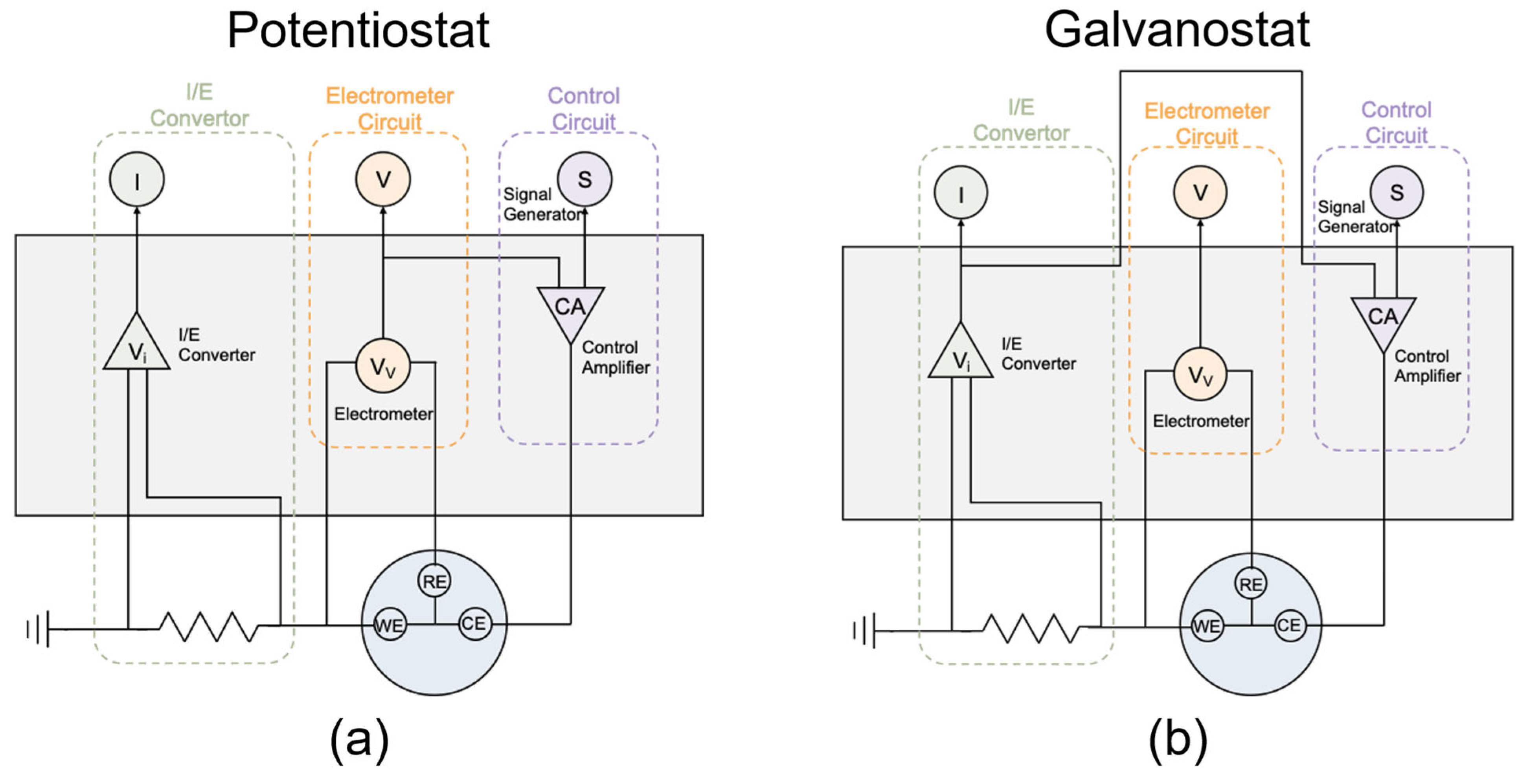
There are several common corrosion protection methods, including coatings, inhibitors, material selection, and cathodic protection [4,5]. Typically, buried pipelines are protected from corrosion threats by coating and CP. CP protects the steel from corrosion through an electrochemical method that converts pipeline metal from an anode to a cathode site by cathodically polarizing the pipeline using a sacrificial anode or impressed current. It was found that impressed current cathodic protection (ICCP) is generally regarded as more effective than sacrificial anode cathodic protection (SACP) in mitigating corrosion due to its flexible voltage and current [2]. Thus, ICCP is commonly used in the field, and the CP values are regulated according to different environmental conditions through potentiostat or galvanostat conditions. For the potentiostat circuit, as shown in Figure 1a, the CP potential signal is generated based on the target and sent to the Control Amplifier. The Control Amplifier applies the signal form to the cell and adjusts its amplitude by comparing the potential tested by the Electrometer and the designed value. In this case, the CP potential is kept at the designed value, and the response of the direct current (DC) density from the I/E Converter is recorded. For the galvanostat circuit, as shown in Figure 1b, the CP current density signal is also generated based on the target value and sent to the Control Amplifier. In this mode, the Control Amplifier adjusts its amplitude based on the current obtained from the I/E Converter and the designed value. Thus, the CP current density is kept at the designed value, and the response of the DC potential from the Electrometer is captured. Both the potentiostat and galvanostat are “external feedback” CP systems, which are easier to monitor in the lab [2]. Understanding the difference between these two circuits (that is how CP is imposed) is important for data interpretation.
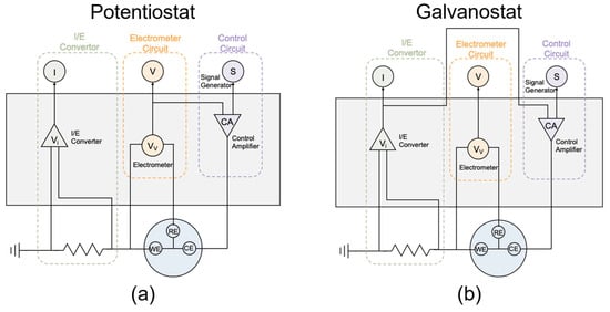
Figure 1.
Schematic diagram of (a) potentiostat and (b) galvanostat circuits.
In addition, many terminologies (especially the electrochemical terms) need to be clarified here first, as it is found that the same quantity may be named differently, or the same term may refer to different quantities in different studies. To avoid confusion, the definitions of the key terminologies are given here:
- CP potential: cathodic protection potential applied on the working electrode (WE) (i.e., pipeline metal).
- CP current density: cathodic protection direct current density flowing through the WE.
- DC potential: real-time actual potential applied to the WE based on the reference electrode (RE) as the feedback of the applied CP current density.
- DC current density: real-time current density flowing through the WE as the feedback of the applied CP potential.
- AC current density: AC current density flowing through the WE
- AC voltage: alternating voltage applied on the WE.
Investigation of AC-induced corrosion of steel dates back to the early 1900s [6]. In 1986, an accident occurred on a polyethylene-coated pipeline in Germany despite implementing standard CP conditions; the PE-coated pipeline was installed parallel to a 16.6 Hz powered railway and equipped with standard CP at the time [7]. This indicates that the steel pipeline under conventional standard CP potential would suffer, at least partially, from corrosion attack under AC interference. Since then, great efforts have been made worldwide to understand AC corrosion of cathodically protected pipelines.
In previous studies, it has been widely reported that AC interference can deviate the potential of the protected pipelines from the applied CP value, even if it meets the conventional CP criteria based on pipe-to-soil potential, a protection potential of −0.850 V vs. CSE [1,2,8,9,10,11,12,13]. For example, Xu et al. [2] reported the DC potential shifted negatively under the standard CP level due to the AC interference. Kuang and Cheng [11] found the DC potential shifted positively when applying a more negative CP level galvanostatically (approximately −1.0 V vs. CSE). Tang et al. [10] also observed a positive shift in the DC potential at a higher level of the applied CP current density (15 A/m2) along with the AC current density. However, a significant shortcoming in most of these studies is the lack of clarity regarding the method of applying CP. It is often not clearly stated whether the CP was applied in potentiostat, galvanostat, or through other “internal feedback” methods. This lack of transparency makes it difficult to compare results across different studies and draw meaningful conclusions. Particularly when using galvanostat to apply the CP current density, some studies used the corresponding DC potential instead of the exact CP current density they applied [2,8,9,11]. Other studies used the exact CP current density but reported a positive current density value [10]. It should be noted that the positive current means positive cathodic current, which implies that the steel loses electrons, accelerating corrosion, which is opposite to the object of cathodic protection. Overall, there is a need to report the testing procedure and data format in a standard way, particularly specifying how CP is applied and the sign of CP or DC data.
Generally, the corrosion rate can be measured using different approaches including, but not limited to, gravimetric analysis (weight loss measurements), electrochemical methods (e.g., Tafel measurements and linear polarization resistance), and non-destructive ultrasonic thickness monitoring [14].
Weight loss measurement is an accurate and reliable method to quantitatively determine the corrosion rate [1], and it has been widely used for studying AC corrosion. Even though many previous studies used weight loss measurements and reported that steel corrosion was accelerated by AC interference [2,8,9,10,11,15,16,17,18,19,20,21,22,23,24,25,26,27,28,29,30,31,32,33], the reliability of the data values obtained from those studies is questionable. For example, most studies did not have any repeated testing for a given condition; some papers used the mounted metal electrode with epoxy for the weight loss measurement, which can introduce large experimental errors; other studies did not provide the details of the weight loss measurement such as the metal coupon.
Tafel measurement is another widely used approach for analyzing corrosion performance [14,22]. In previous studies, polarization curves under AC interference have been measured, and it was observed that AC current density had a slight effect on the cathodic reaction but had a significant influence on the anodic reaction [22]. However, there is a lack of studies on cathodically protected steel under AC interference using Tafel. The Tafel measurement is a quick testing method to monitor the corrosion behavior of the system based on applying a linear potential sweep from −250 mV to +250 mV relative to corrosion potential. The data can be used to study the corrosion rate and corrosion mechanism. The use of Tafel measurement provides a new insight to forecast and evaluate the AC-induced corrosion of buried pipelines. It is challenging in the experimental setup to measure the Tafel measurement along with the introduction of CP and AC. That could be the reason for a lack of studies here.
In this study, we make multiple improvements to address the issues of various shortcomings and uncertainties in the previous research we mentioned above. First, this paper will clearly describe how cathodic protection is applied and use negative values to represent the applied CP current density on the metal. Second, the exact weight loss coupons were used, and each condition was repeated at least three times to minimize experimental errors and improve accuracy, rectifying the inaccuracies that might have occurred due to insufficient repetitions previously. Finally, the Tafel measurement was employed to obtain an additional set of corrosion rate values for steels under various CP levels and AC interference. This method can mutually validate the corrosion rates obtained from weight loss measurements, thereby strengthening the credibility of the research findings and filling the gap in the lack of cross-validation in previous works.
To understand the effectiveness of cathodic protection under AC interference, this study investigated the corrosion behavior of C1018 and API 5L X60 steels under different levels of cathodic protection with AC interference. The cathodic protection was applied on the steel either galvanostatically or potentiostatically. Both weight loss measurements and Tafel measurements were used to analyze the corrosion rate of two types of steel. Probabilistic models were developed based on the experimental data obtained to predict the corrosion rate from the two measurement methods while accounting for uncertainty in the corrosion rate measurements. The sensitivity of each model to variations in the values of random variables was also assessed.
2. Materials and Methods
2.1. Metals
In this study, two types of metal, C1018 steel and API 5L X60 steel, were purchased from McMaster Carr (Aurora, OH, USA) and Metal Sample Company (Munford, AL, USA), respectively. The chemical compositions of these two metals are presented in Table 1.

Table 1.
Chemical composition and yield strength of the metal in the investigation.
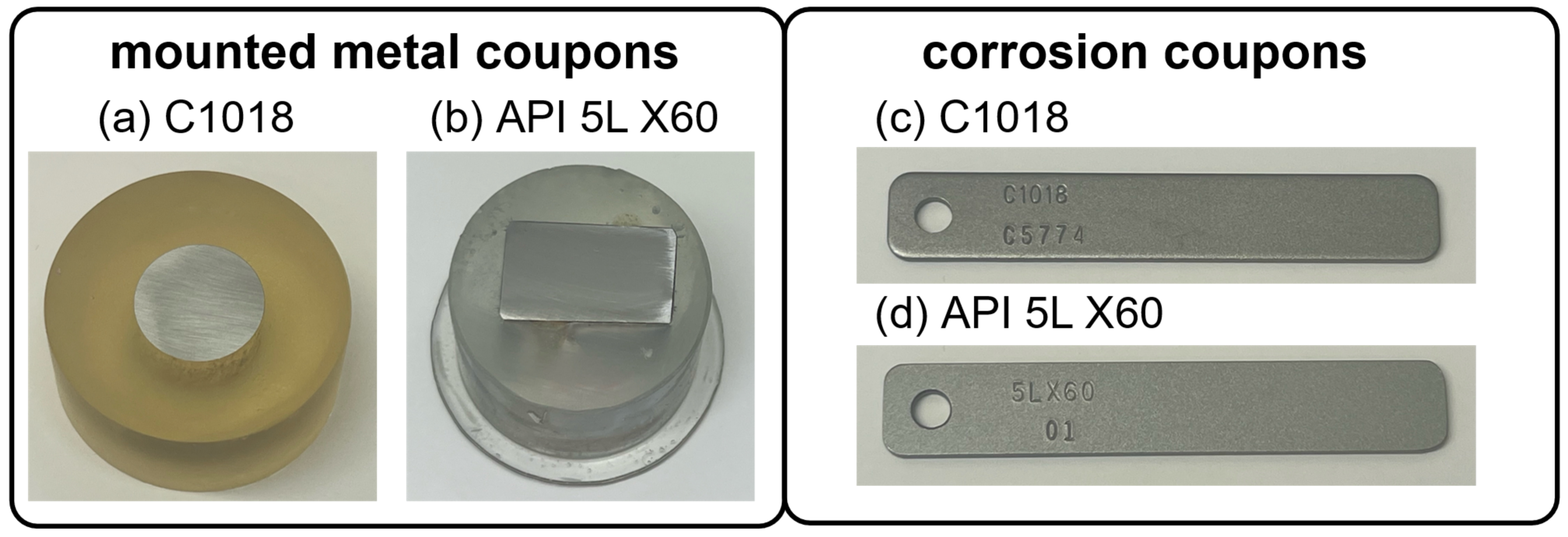
Two types of testing coupons were produced for each of these metal types, mounted metal coupons and corrosion coupons, as shown in Figure 2. The mounted metal coupons (Figure 2a,b) were used for electrochemical measurements, including potentiostat, galvanostat, and Tafel. A copper wire was welded to the back of each cut metal sample to serve as the working electrode. Subsequently, the metals were meticulously sealed with epoxy, ensuring no grooves or bubbles at the epoxy/steel interface. To achieve a smooth and uniform surface, the mounted steel surfaces were polished using 240, 400, 600, 800, and 1200 grit sandpapers, resulting in a mirror-like finish free from scratches. Then, the working area of each specimen was maintained at 2 cm2 with Gamry portHole electroplating tape.
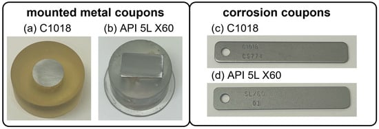
Figure 2.
Photos of metal samples: (a) mounted C1018 metal coupon; (b) mounted API 5L X60 metal coupon; (c) C1018 weight loss corrosion coupon; (d) API 5L X60 weight loss corrosion coupon.
The corrosion coupons, shown in Figure 2c, with dimensions of 3″ × 0.5″ × 0.063″, were used for weight loss measurements. Prior to testing, the specimens underwent a thorough cleaning process using distilled water and acetone to ensure their cleanliness.
2.2. Chemical Composition of the Solution
The test solution used in this study was a simulated soil solution consisting of 8.933 g/L KCl (99%), 1.170 g/L MgSO4∙7H2O (98%), and 5.510 g/L NaHCO3 (100%), with a pH of 8.08 and a conductivity of 20.0 mS/cm. The testing solution was designed considering the major elements in soils and following previous studies on the simulated solutions [9]. The KCl (99%), MgSO4∙7H2O (98%), and NaHCO3 (100%) were purchased from Sigma-Aldrich, Fisher, and VWR chemicals, respectively. All solutions were prepared from analytic-grade reagents and deionized water. All experiments were conducted at room temperature (~22 °C) and open to the air.
2.3. Experimental Setup
The schematic diagram of the experimental setup is shown in Figure 3, including an AC circuit and a DC circuit. The DC circuit was executed by the Gamry Reference 600+ working station (working station 1) with a three-electrode system consisting of a mounted metal coupon (Figure 2) as the working electrode (WE), a saturated calomel as the reference electrode (RE), and a platinum sheet as a counter electrode (CE). In the AC circuit, a constant sine-wave AC with a frequency of 60 Hz was applied by the Virtual Front Panel (VFP) via another Gamry Reference 600+ working station (working station 2). The inductor element was designed to prevent the AC from leaking into working station 1. Also, working station 2 has built-in capacitor components to block the DC signals. The experimental testing cell with AC and DC circuits is shown in Figure 4.
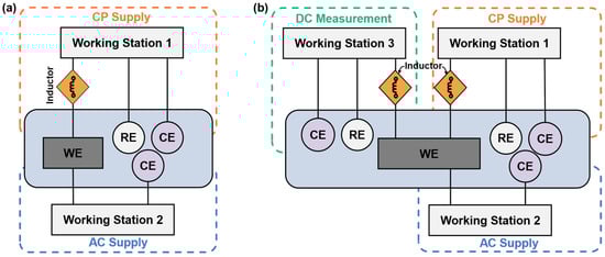
Figure 3.
(a) Schematic diagram of the electrochemical measurement and weight loss measurement of the steel under various AC and CP conditions. (b) Schematic diagram of Tafel measurement of the steel under various AC and CP conditions.
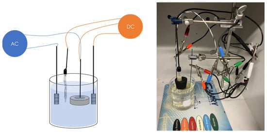
Figure 4.
AC corrosion experimental setup including a schematic diagram and a photograph of the AC and DC circuit.
This study used two methods to apply cathodic protection: galvanostat and potentiostat. The galvanostat applies a fixed CP current density on the working electrode, with DC potential as a response. The potentiostat applies a constant CP potential on the working electrode, with a change in DC current density as its feedback. All the feedback parameters were recorded by the Gamry Reference 600+ working station for analysis.
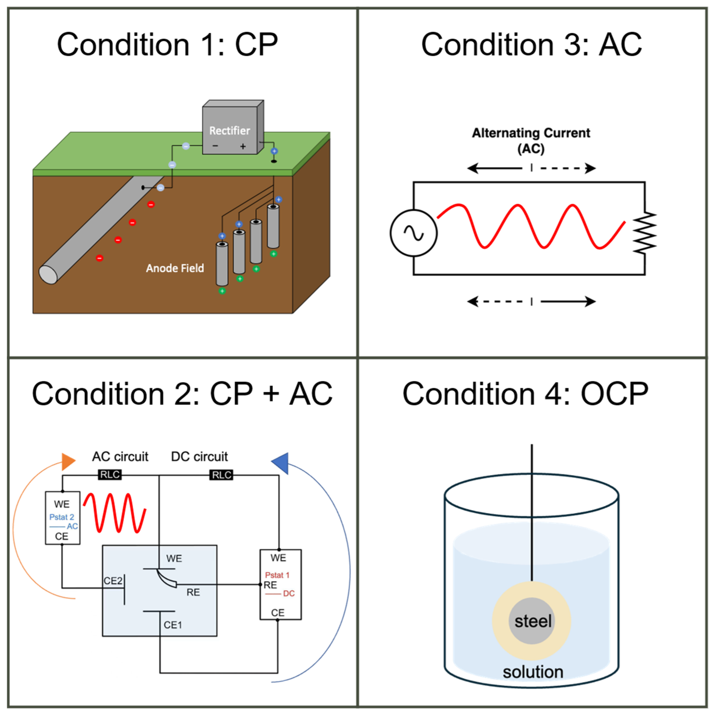
To study the effectiveness of cathodic protection under AC interference, the cathodic protection experiment was designed to have four conditions: steel under CP, steel under CP with AC interference (i.e., CP + AC), steel under AC interference without CP (i.e., AC), and steel without any external input (i.e., OCP), as demonstrated in Figure 5. This division facilitated a comprehensive analysis of CP effectiveness under various conditions, including the influence of CP levels, AC levels, and their combinations.
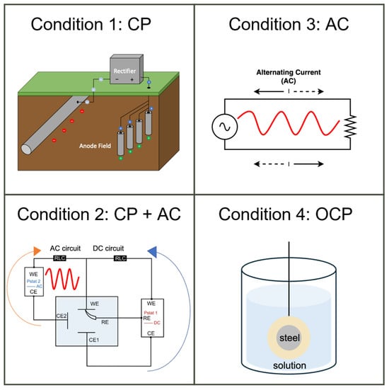
Figure 5.
Four experimental conditions for electrochemical measurements and corrosion rate tests.
2.4. Corrosion Rate Tests
The corrosion rate is a crucial and straightforward parameter used to evaluate the durability of a metal and estimate its expected lifespan in a particular environment. It provides valuable insights into the corrosion behavior of metal components or structures. Various methods are available to measure corrosion rate, including weight loss, weight gain, thickness measurements, and electrochemical measurements [14,34,35]. In this experiment, Tafel measurement and weight loss measurement were used to determine the corrosion rate of C1018 and X60 steels under the 4 conditions mentioned in Figure 5, which aids in understanding the effectiveness of cathodic protection of the steels under varying AC conditions. At least three samples were tested under each condition.
2.4.1. Tafel Measurement
Tafel measurement is a technique that involves applying a voltage sweep to a metal and measuring the current feedback. The method provides information about the corrosion potential and corrosion current density, which can be used to calculate the corrosion rate based on Equation (1):
where CR is corrosion rate, mpy (mils per year); is corrosion current density, μA/cm2; is the equivalent weight of the corroding species, g; is the density of the corroding species, g/cm3.
The experiment setup for Tafel measurement is shown in Figure 3b. The Tafel was conducted in parallel with CP, AC, or CP and AC. The corrosion rate of various conditions was tested using the Tafel mode of Gamry Reference 600+ equipment. The potential sweep ranged from −0.2 to 0.2 V relative to the open circuit potential (OCP), with a scan rate of 0.2 mV/s. Before conducting the potential sweep, the OCP of the working electrode was measured for at least half an hour to ensure it reached a stationary value. The Tafel measurement was used after the OCP to obtain the corrosion potential and corrosion current density. Finally, based on the parameters obtained from Tafel, the corrosion rate can be calculated using Equation (1).
2.4.2. Weight Loss Measurement
The experimental setup for weight loss measurement is shown in Figure 3a. The weight loss corrosion coupons were cleaned according to the ASTM G1 standard and weighed before the test. Subsequently, they were immersed in the test solution under 4 different conditions (Figure 5) for 72 h.
Afterward, the corrosion product formed on the surface of the coupons was carefully removed using mechanical and chemical methods. Mechanical methods, including light scraping and scrubbing, were used to remove tightly adherent corrosion products. The chemical cleaning procedure of ASTM G1 was followed and repeated several times to remove the corrosion product thoroughly. The weight of the steel coupon was measured by Mettler Toledo ML104 analytical balance with an accuracy of 0.1 mg. The weight loss of the steel can be used to calculate the corrosion rate based on Equation (2):
where is corrosion rate, mpy (mils per year); W0 and W are the weight of the specimen before and after the experiment with the removal of corrosion products, g; S is the exposed area, cm2; t is the corrosion time, h; and is the density of the specimen, g/cm3. At least three duplicated samples were tested for each condition to obtain an average value.
3. Results
3.1. Real-Time Feedback of DC Current Density When Applying CP Potential
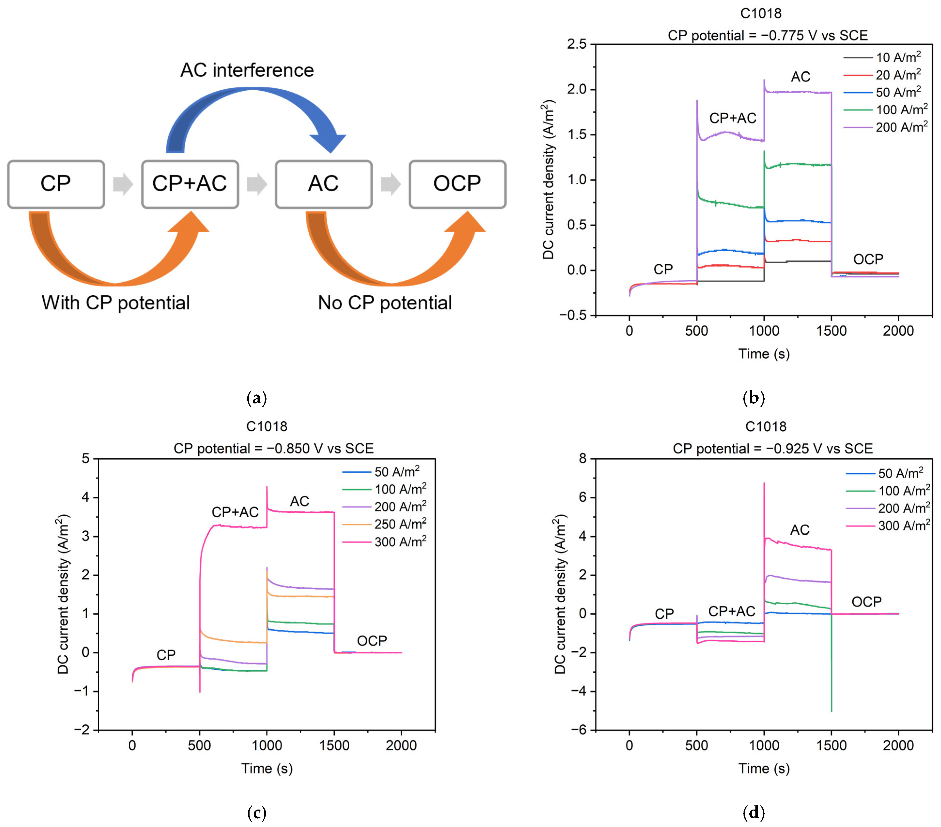
The cathodic protection was applied via a potentiostat circuit (Figure 1a) to keep a constant value of the CP potential to the metal. Figure 6b–d depict the real-time feedback of the DC current density when applying the CP potential. Three different levels of CP potential, i.e., −0.775, −0.850, and −0.925 V vs. SCE, were applied to C1018 steel under various AC current densities. As shown in Figure 6a, the entire process can be divided into four stages, corresponding to the four conditions mentioned in Figure 5. The testing time for each stage was 500 s to ensure the DC current density achieved a steady state under each condition, resulting in a total of 2000 s for the four stages.
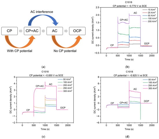
Figure 6.
(a) Schematic diagram of 4 stages of cathodically protected C1018 steel under AC interference; DC current densities during the 4 stages with different CP potentials and AC current densities: (b) CP potential of −0.775 V vs. SCE; (c) CP potential of −0.850 V vs. SCE; (d) CP potential of −0.925 V vs. SCE.
Real-time changes in DC current density across the four stages are shown in Figure 6b–d. The OCP condition (i.e., the fourth stage) refers to a steady-state, freely corroding condition. The potential is called the open-circuit potential or corrosion potential, and there is no net current flow, which means that the DC current density is 0 A/m2 [14]. Under other conditions, the DC current density can be categorized as either anodic current density if the current is positive, or cathodic current density if it is negative [2,9,10,11,36]. Anodic current density occurs when the net rate of iron dissolution is faster than the net rate of hydrogen evolution, indicating a significant metal loss. On the other hand, cathodic current density represents the opposite situation where the corrosion of metal slows down [14].
In Figure 6b–d, cathodic DC current densities are observed in the CP condition (i.e., the first stage) at the three levels of CP potentials. The observation is consistent with previous research that the cathodic DC current density was generated when applying CP [2,11]. This observation indicates that the metal was protected at these CP potentials. However, anodic DC current densities were observed in the AC condition (i.e., the third stage) even when the AC current density was 10 A/m2. The AC stage has been scarcely investigated in previous studies, yet it could potentially offer valuable insights into the influence of AC on metal corrosion. This observation suggests that the steel behaved as an anode under AC, indicating AC-induced corrosion.
When the applied CP potential was −0.775 V vs. SCE (Figure 6b), anodic DC current densities were observed in the CP + AC condition (i.e., the second stage). This indicates that the rate of iron dissolution accelerated compared to the OCP condition (i.e., the fourth stage) and the introduction of AC current density exacerbated the severity of corrosion. Moreover, the generation of anodic DC current density implies the AC current density shifted the DC current density from the cathodic to the anodic regime. Additionally, the anodic DC current density increased with the rise in AC current density. The same shift direction of DC current density was reported in previous research [2,11]. These observations collectively indicate that AC leads to more severe corrosion even when applying CP potential. Furthermore, the presence of AC appears to diminish the effectiveness of the CP potential of −0.775 V vs. SCE, and higher AC current densities exhibited a greater ability to counteract the protective effect of the CP potential.
When the applied CP potential was −0.850 V vs. SCE (Figure 6c), an anodic DC current density was observed in the CP + AC condition when AC current densities were larger than 200 A/m2. Conversely, cathodic DC current density was recorded in the CP + AC condition when AC current densities were smaller than 200 A/m2. Thus, the CP potential of −0.850 V vs. SCE is incapable of protecting C1018 steel from AC corrosion when AC current density exceeds 200 A/m2. Analogous findings were reported when the CP potential was −0.850 vs. SCE, wherein the application of higher AC current densities was associated with the presence of anodic DC current density, while the imposition of lower AC current densities correspondingly resulted in cathodic DC current density [11].
When the applied CP potential was −0.925 V vs. SCE (Figure 6d), only cathodic DC current density was observed in the CP + AC condition for all AC levels. This indicates that the net rate of iron dissolution was diminished under a CP potential of −0.925 V vs. SCE. Consequently, the corrosion of the metal was slowed. It is noted that the cathodic DC current density increased to a more negative value as the AC current density increased. This trend has also been reported in previous papers [2,11]. Therefore, this CP level appears to slow the corrosion of the metal, even in the presence of AC interference. Overall, the real-time DC current densities help us better understand the corrosion behavior of steel under different AC and CP conditions. In the CP condition (i.e., the first stage), the rate of steel dissolution slowed down, and the steel was protected. In AC conditions (i.e., the third stage), the rate of steel dissolution increased, and the corrosion of steel accelerated. In the CP + AC condition (i.e., the second stage), the DC current density was determined by the mutual interaction of the applied CP potential and the level of AC interference. When the CP potential was at a low level (−0.775 V vs. SCE), the corrosion of the steel was accelerated even by small AC interference. When the CP potential was at a medium level (−0.850 V vs. SCE), the corrosion of steel slowed under a low-level AC current density, but it accelerated under a high-level AC current density. When the CP potential was at a high level (−0.925 V vs. SCE), the steel dissolution slowed down even when the AC current density was as high as 300 A/m2. These findings highlight the importance of AC and CP levels in corrosion processes. Therefore, the lack of consideration of AC interference in CP standards can potentially lead to misleading results, especially when metals are exposed to high levels of AC.
3.2. Real-Time Feedback of DC Potential When Applying CP Current Density
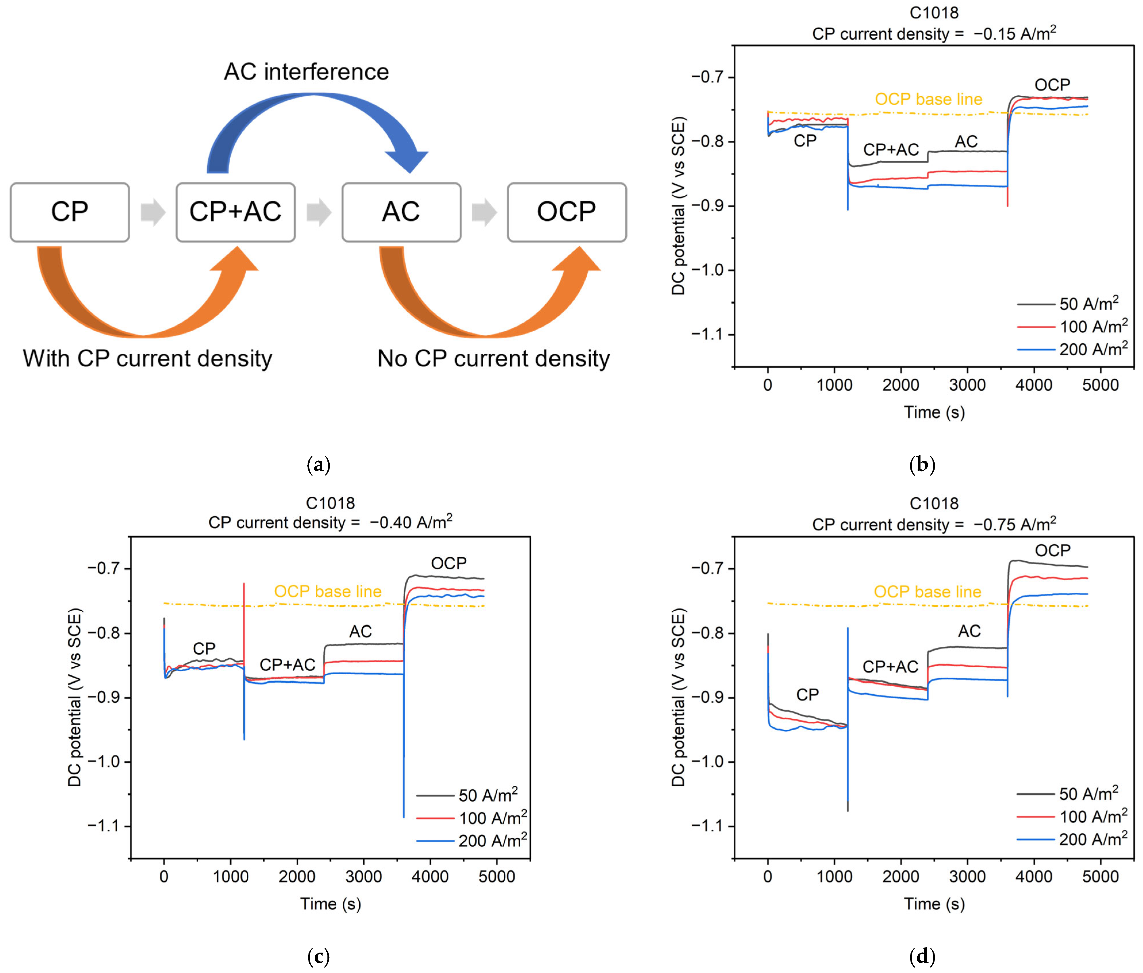
The cathodic protection was applied via a galvanostatic circuit (Figure 1b) to keep a constant value of a CP current density applied to the metal. Figure 7b–d illustrate the real-time feedback of the DC potential of C1018 steel under different AC and CP current densities of −0.15, −0.40, and −0.75 A/m2, respectively. As shown in Figure 7a, the entire process can be divided into four stages. These four stages correspond to the four conditions mentioned in Figure 5. The testing time for each stage was 1200 s to ensure the DC potential achieved the steady state under each condition, resulting in a total of 4800 s for the four stages. Real-time DC potential changes were observed across the four stages as shown in Figure 7b–d. In the CP condition (i.e., the first stage), when a CP current density of −0.15 (Figure 7b), −0.40 (Figure 7c), or −0.75 A/m2 (Figure 7d) was applied, the DC potential gradually reached approximately −0.775, −0.850, or −0.925 V vs. SCE, respectively. All the DC potential values in the first stage were more negative than the open circuit potential (OCP).
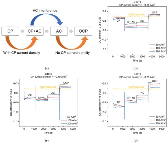
Figure 7.
(a) Schematic diagram of 4 stages of cathodically protected C1018 steel under AC interference; DC potential during the 4 stages with different CP and AC current densities: (b) CP current density of −0.15 A/m2; (c) CP current density of −0.40 A/m2; (d) CP current density of −0.75 A/m2.
In the OCP condition (i.e., the fourth stage) depicted in Figure 7b–d, the DC potential immediately shifted positively and gradually reached a steady value. This steady value was different than the OCP of the metal because this OCP was tested after AC and CP conditions, which may influence the oxidation reactions that may contribute to the OCP value. Additionally, there were some fluctuations of the DC potential under different AC current densities in the OCP stage, which is also related to the contributions of oxidation reactions by previous residual effects from AC. Similar phenomena were also reported in previous studies [2,8,9,10,11].
In the AC condition (i.e., the third stage) depicted in Figure 7b–d, the DC potential values were −0.825, −0.850, and −0.875 V vs. SCE under AC current densities of 50, 100, and 200 A/m2, respectively, all of which were more negative than the OCP. Similar observations were reported in previous studies [8,9,11].
In the CP + AC condition (i.e., the second stage), when CP current density was −0.15 A/m2 (Figure 7b) and −0.40 A/m2 (Figure 7c), the DC potential shifted in the negative direction when AC current density was introduced to the CP current density. Furthermore, the larger the AC current density, the more negative shift in the DC potential. However, when a CP current density of −0.75 A/m2 (Figure 7d) was applied, the DC potential shifted in a positive direction under AC interference. Compared to the DC potential in the OCP condition, all the DC potentials in the CP + AC condition were more negative than those in the OCP condition.
According to the basis of the corrosion, a negative potential indicates that the metal gains electrons and behaves as a cathode, which is generally protected against corrosion [14]. However, as discussed in Section 3.1, the corrosion occurred under AC interference demonstrated from the anodic current density, even though the DC potential was lower than the OCP under AC interference (Figure 7b–d). Therefore, the potential shift cannot be viewed as the only parameter to determine or evaluate AC corrosion due to its complexity. It is necessary to measure the exact corrosion rate of a metal under different CP and AC conditions.
3.3. Corrosion Rate by Weight Loss Measurement
The corrosion rate of two types of metals, C1018 and API 5L X60, under cathodic protection and AC interference, was measured after 3 days of weight-loss testing in the simulated solution. Figure 8, Figure 9, Figure 10 and Figure 11 show corrosion rates of C1018 and API 5L X60 by scatter column charts with error bars under different AC and CP current densities, respectively.
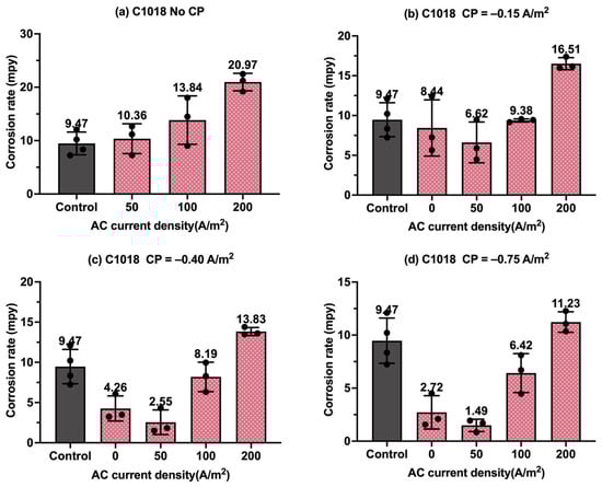
Figure 8.
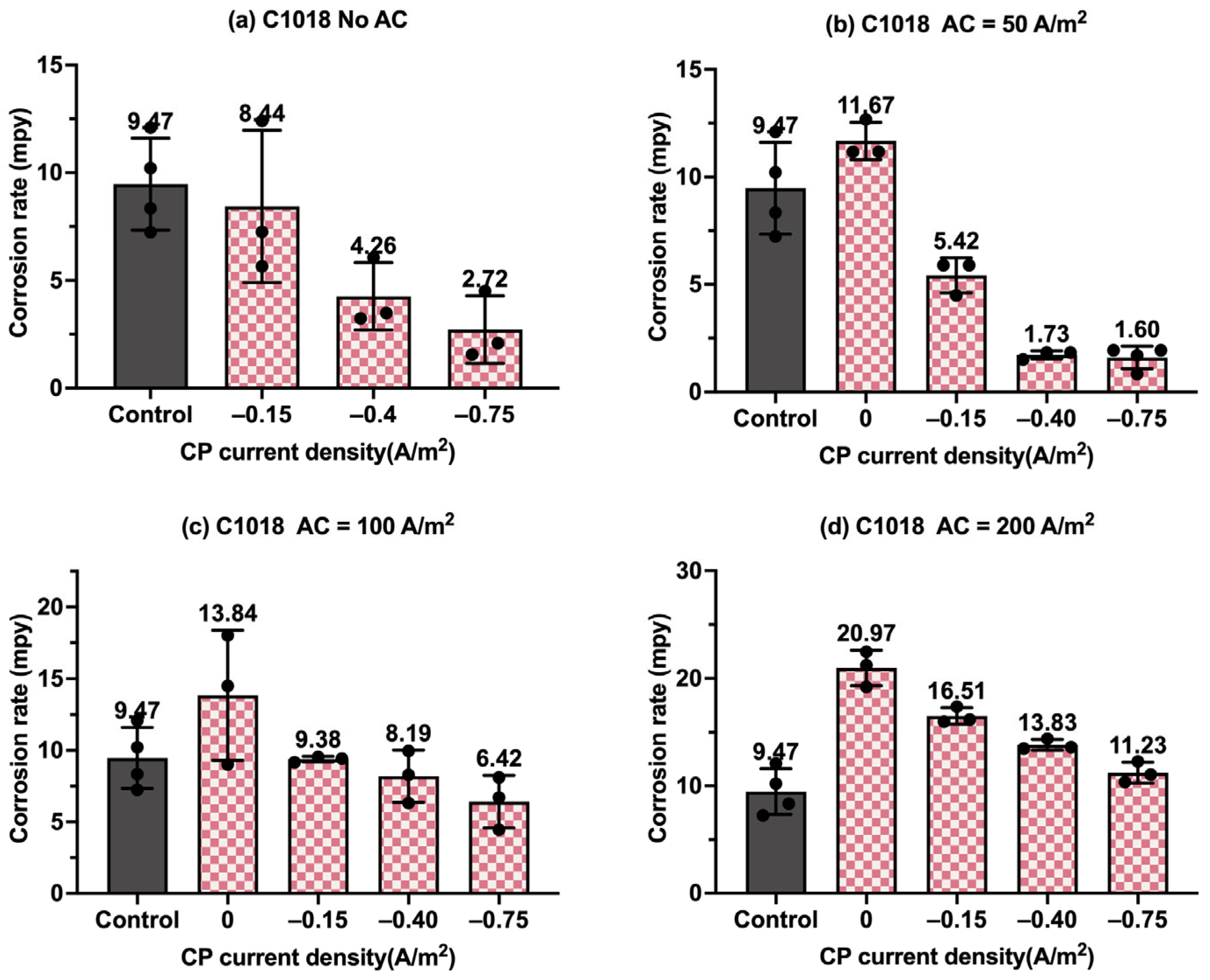
Corrosion rate of C1018 steel under various AC and CP conditions by weight loss measurement: (a) no CP; (b) CP current density of −0.15 A/m2; (c) CP current density of −0.40 A/m2; (d) CP current density of −0.75 A/m2. The control group is shown in each subfigure to illustrate the natural corrosion rate without AC and CP.
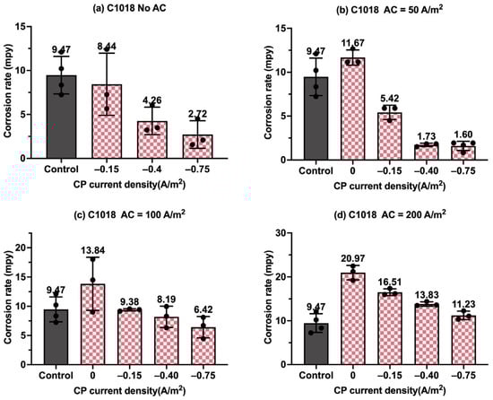
Figure 9.
Corrosion rate of C1018 steel under various AC and CP conditions by weight loss measurement: (a) no AC; (b) AC current density of 50 A/m2; (c) AC current density of 100 A/m2; (d) AC current density of 200 A/m2. The control group is shown in each subfigure to illustrate the natural corrosion rate without AC and CP.
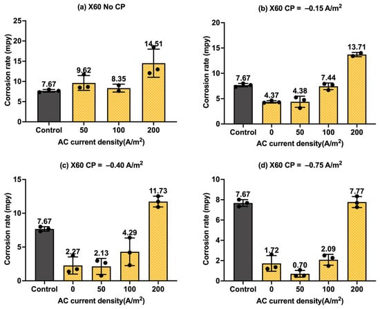
Figure 10.
Corrosion rate of API 5L X60 steel under various AC and CP conditions by weight loss measurement: (a) no CP; (b) CP current density of −0.15 A/m2; (c) CP current density of −0.40 A/m2; (d) CP current density of −0.75 A/m2. The control group is shown in each subfigure to illustrate the natural corrosion rate without AC and CP.
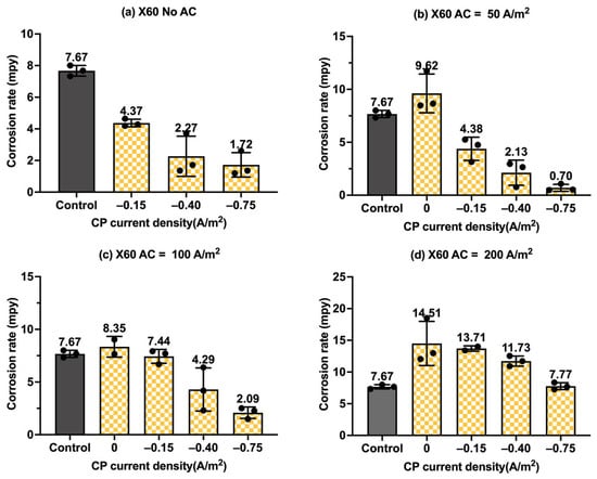
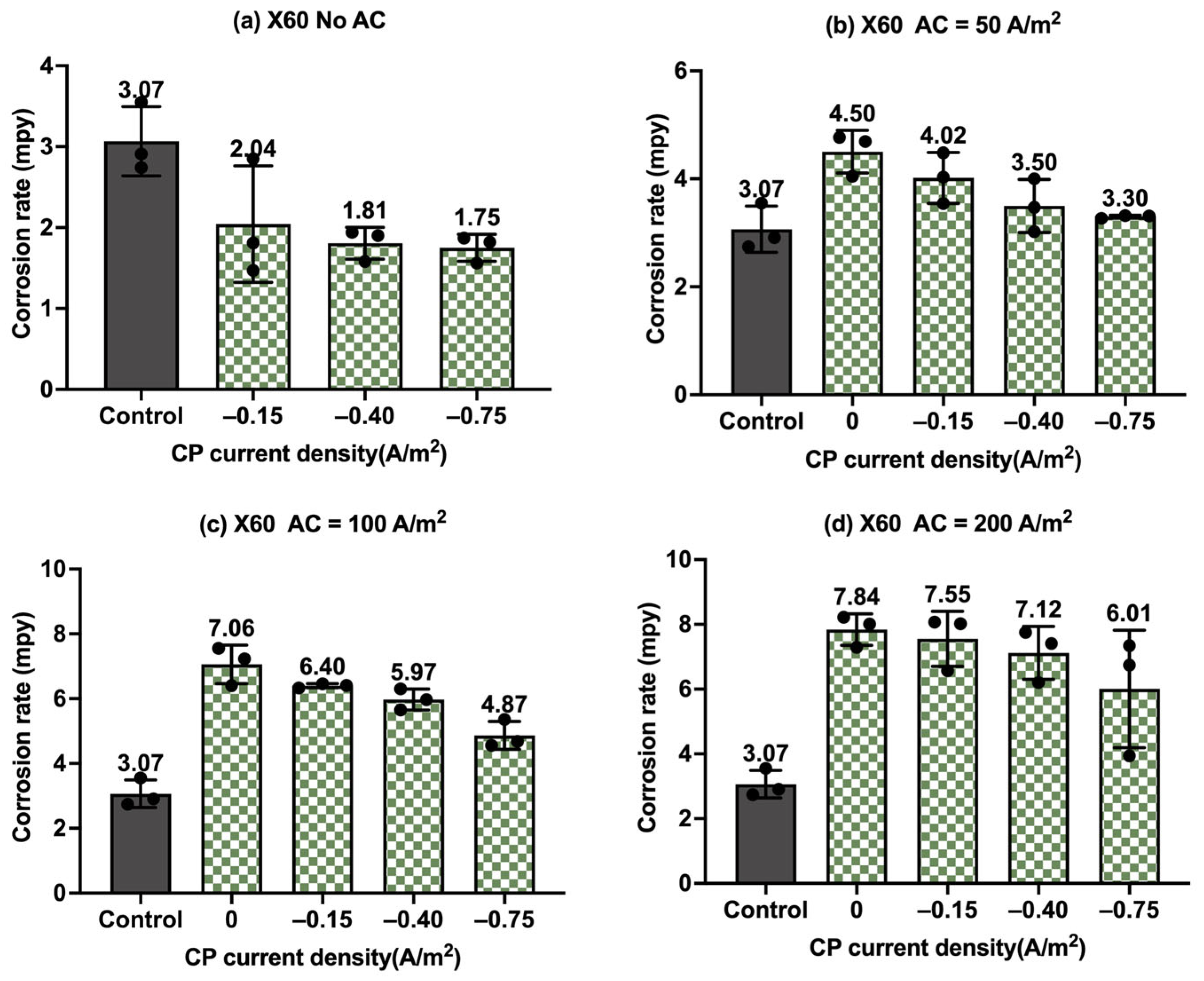
Figure 11.
Corrosion rate of API 5L X60 steel under various AC and CP conditions by weight loss measurement: (a) no AC; (b) AC current density of 50 A/m2; (c) AC current density of 100 A/m2; (d) AC current density of 200 A/m2. The control group is shown in each subfigure to illustrate the natural corrosion rate without AC and CP.
Figure 8 shows the corrosion rate of C1018 steel under four different levels of CP and AC current density values, in which the gray columns are related to the control samples, i.e., the samples under a freely corroding condition (no CP and no AC), with an average corrosion rate of 9.47 mpy obtained by weight loss measurement. As shown in Figure 8a, the corrosion rate increased as the AC current density increased. Figure 8b–d show the corrosion rate of the C1018 steel under cathodic protection while introducing AC current density. When the CP current density was −0.15 A/m2, the corrosion rate was comparable to or smaller than that of the control samples when the AC current density was smaller than 100 A/m2; however, the corrosion rate significantly increased when the AC current density was 200 A/m2. This phenomenon demonstrates that this CP level is insufficient for cathodic protection when the AC current density is 200 A/m2 or larger. For the other two CP levels, a similar trend was observed as AC current density was increased from 0 to 200 A/m2.
Figure 9 presents the corrosion rate of C1018 metals in another form to clearly demonstrate the effectiveness of the cathodic protection under AC interference. Figure 9a shows the corrosion rate of C1018 metals under cathodic protection without introducing AC interference. The corrosion rate decreased with the increase in the CP current densities, which clearly demonstrates that the effectiveness of cathodic protection was enhanced by increasing the CP levels. When AC current was introduced at the level of 50 A/m2, as shown in Figure 9b, the corrosion rate rose under no cathodic protection, but it dropped substantially when CP current density was introduced, demonstrating the effective cathodic protection when the AC current density was at the level of 50 A/m2. A similar trend can be seen in Figure 9c when the AC current density was 100 A/m2. However, as shown in Figure 9d, when the AC current density was increased to 200 A/m2, all the corrosion rates were higher than that of the control sample for all three levels of CP current density, which means the applied cathodic protection current densities were ineffective when the AC current density was 200 A/m2 or larger.
Figure 10 shows the corrosion rate of API 5L X60 steel under four different levels of AC and CP current density values, where Figure 10a corresponds to the corrosion rate without cathodic protection. The gray columns refer to the control sample under the freely corroding condition, where the average corrosion rate was 7.67 mpy, 1.8 mpy smaller than the corrosion rate of C1018 under the same condition. Obviously, the corrosion rate increased with the increase in the AC current density, and it was higher than that of the control samples. Figure 10b–d show the corrosion rate of the API 5L X60 steel under cathodic protection while introducing AC interference. When the CP current density was −0.15 A/m2, the corrosion rate was comparable to or smaller than that of the control samples when the AC current density was smaller than 100 A/m2; however, the corrosion rate significantly increased when the AC current density was 200 A/m2, which shows a similar trend to that of the C1018 steel. This phenomenon demonstrates that this CP level was insufficient for effective cathodic protection when the AC current density was 200 A/m2 or larger. For the other two CP levels, a similar trend was observed when the AC current density was increased from 0 to 200 A/m2. This observation was the same as that of C1018, as shown in Figure 8.
Moreover, Figure 11 shows the corrosion rates of API 5L X60 steel under different levels of CP and AC current densities in another format, providing clear insights into the effectiveness of cathodic protection. Figure 11a shows the corrosion rate of API 5L X60 steel under different levels of cathodic protection without AC interference. It clearly shows a decrease in corrosion rate with CP current density, indicating the enhanced effectiveness of cathodic protection at higher CP levels. When AC current density at a level of 50 A/m2 (Figure 11b) and 100 A/m2 (Figure 11c) was introduced, the corrosion rate increased in the absence of cathodic protection, but it decreased substantially when CP current density was applied. This clearly indicates that the cathodic protection was effective in mitigating corrosion when the AC current density was smaller than 100 A/m2. However, as shown in Figure 11d, when the AC current density reached 200 A/m2, the corrosion rate was not reduced under three different levels of cathodic protection. This implies that the CP current density of −0.75 A/m2 became ineffective when AC current density reached 200 A/m2 or higher. A similar observation was made for C1018 steel in Figure 9.
Observations from the weight loss results for C1018 and API 5L X60 indicate that an increased AC current density can lead to a higher corrosion rate. Conversely, a more negative CP current density can have a more protective effect against corrosion, even with AC interference. These findings align with the trend in Figure 6 revealed by the potentiostat and contrast with the observations in Figure 7 from the galvanostat. This observation makes us realize that relying on DC potential alone may lead to a misunderstanding of AC corrosion.
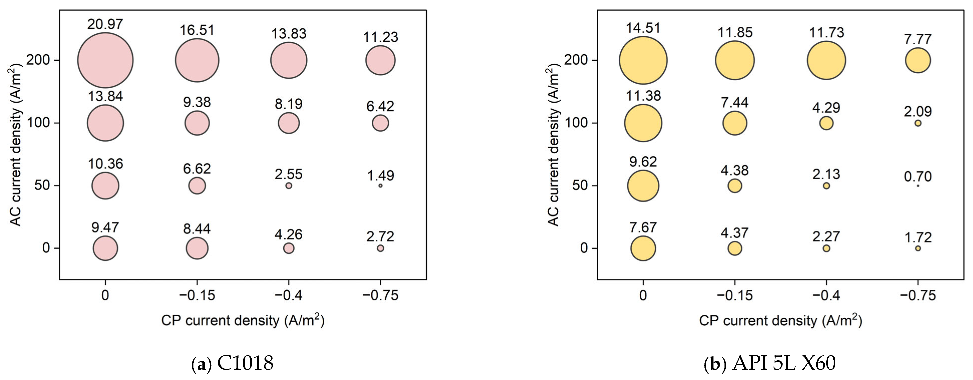
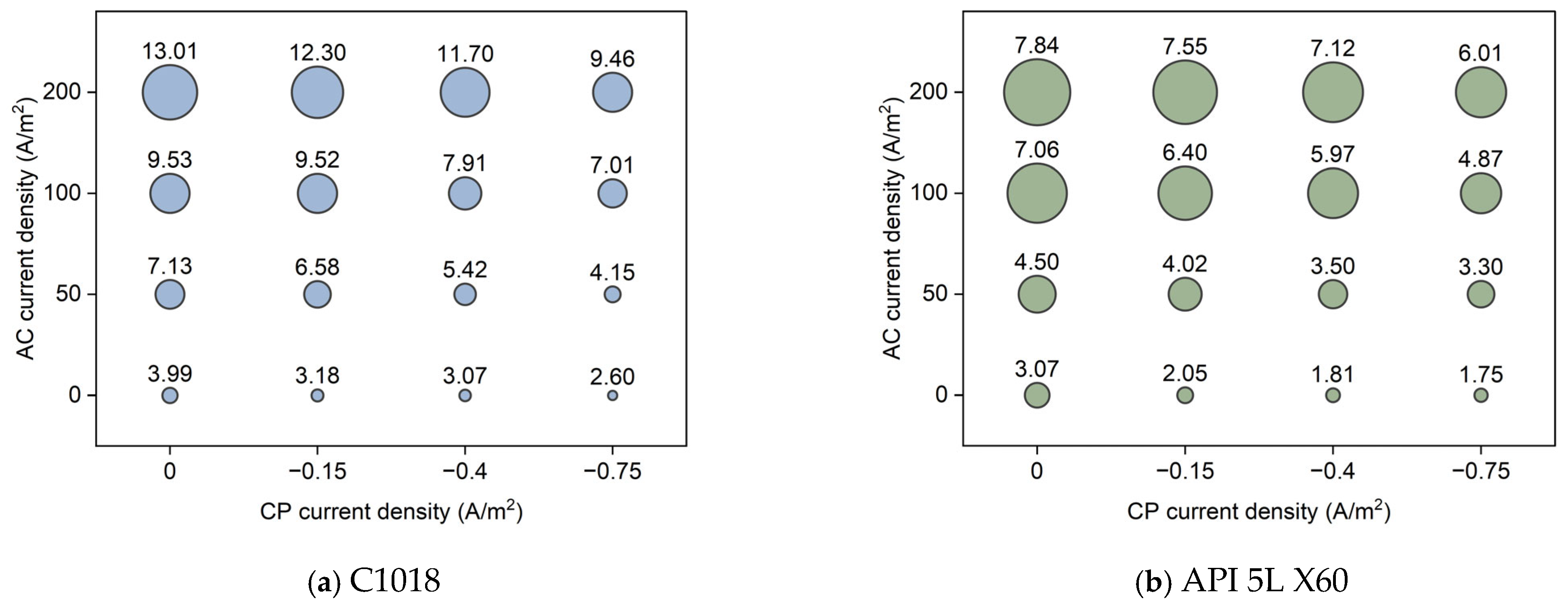
Figure 12 shows the average corrosion rate of C1018 and API 5L X60 metals under different conditions of AC and CP current densities. The size of the bubble corresponds to the average corrosion rate. Obviously, the highest corrosion rate value was obtained under high AC current density without cathodic protection. In fact, the higher the AC current density, the higher the corrosion rate; also, the higher the CP current density, the lower the corrosion rate. In addition, it is shown that the CP current density of −0.75 A/m2 was insufficient for cathodic protection when the AC current density was 200 A/m2, as it resulted in higher corrosion rate values than the control samples. However, the CP current density of −0.75 A/m2 could reduce the effect of high AC interference (200 A/m2) by 46% (from 20.97 mpy to 11.23 mpy for C1018, from 14.51 mpy to 7.77 mpy for API 5L X60). Under low AC interference (50 A/m2), the CP current density of −0.75 A/m2 was far more effective, reducing corrosion rate by 86% for C1018 (from 10.36 mpy to 1.49 mpy) and 93% for API 5L X60 (from 9.62 mpy to 0.70 mpy), respectively. It is noted that the corrosion rate of API 5L X60 was lower than that of C1018 steel under the same condition. This explains why API 5L X60 is one of the most commonly used pipelines in the field due to its better corrosion resistance [37].
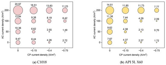
Figure 12.
The corrosion rate of (a) C1018 steel and (b) API 5L X60 under various AC and CP conditions by weight loss measurement. The corrosion rate values are in mpy.
3.4. Corrosion Rate by Tafel Measurement
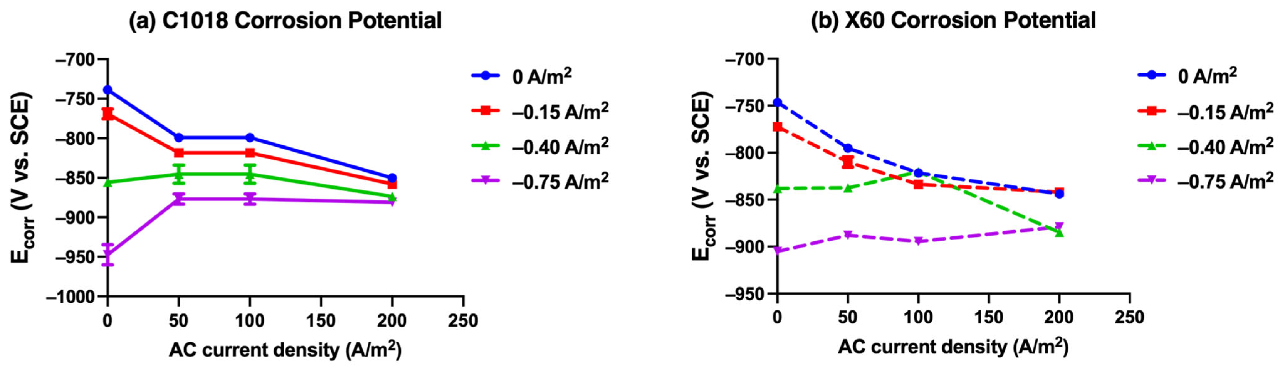
The corrosion rates of C1018 and API 5L X60 steel were tested through Tafel measurements under all the conditions mentioned in Figure 5. Tables S1 and S2 present the kinetic parameters derived from the Tafel plot for C1018 and X60, respectively. It includes corrosion potential (Ecorr), average cathodic Tafel slope (), average anodic Tafel slope (), average corrosion current density (Icorr), and the calculated average corrosion rate in mpy. The Tafel slope parameters did not show an obvious trend under different AC and CP conditions. Also, all the Tafel plots did not demonstrate a shape change which means no new corrosion mechanism was generated. The corrosion potential results for C1018 and X60 steel are plotted in Figure 13 using a line plot with mean and error. The results of the corrosion rate are plotted in Figure 14, Figure 15, Figure 16, Figure 17 and Figure 18 through bubble charts and scatter column charts with error bars, emphasizing different aspects of the relationship between corrosion rate and AC and DC current densities.
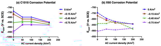
Figure 13.
The corrosion potential derived from Tafel plots for (a) C1018 and (b) X60 steel immersion in simulated soil solution at 25 °C under various AC and CP conditions.
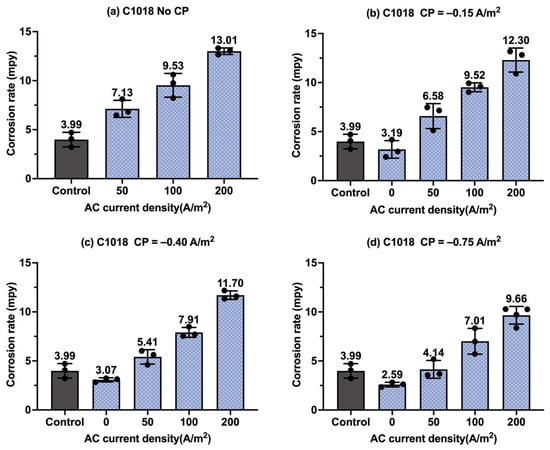
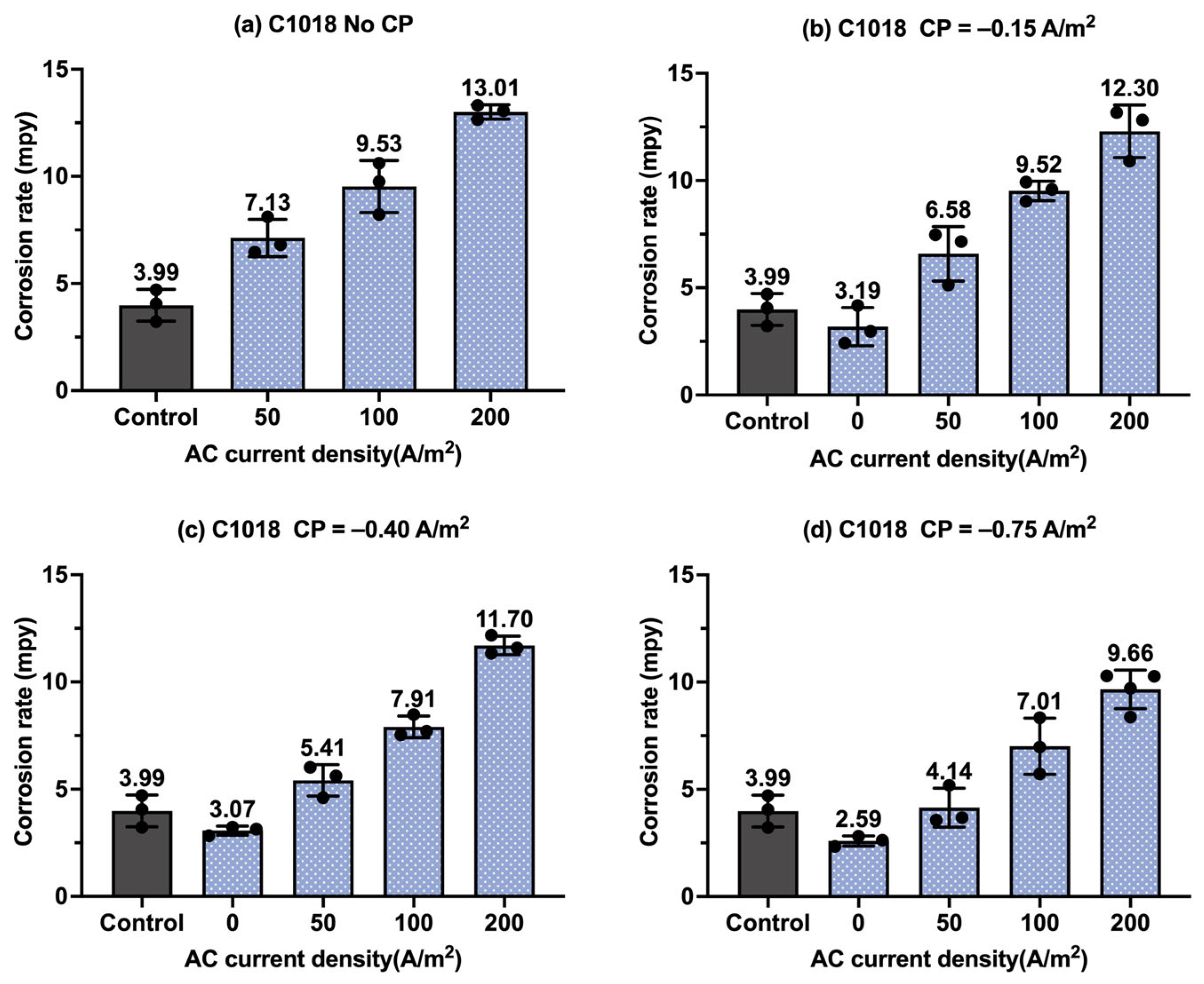
Figure 14.
The corrosion rate of C1018 steel under various AC and CP conditions by Tafel measurements: (a) no CP; (b) CP current density of −0.15 A/m2; (c) CP current density of −0.40 A/m2; (d) CP current density of −0.75 A/m2. The control group is shown in each subfigure to illustrate the natural corrosion rate without AC and CP.

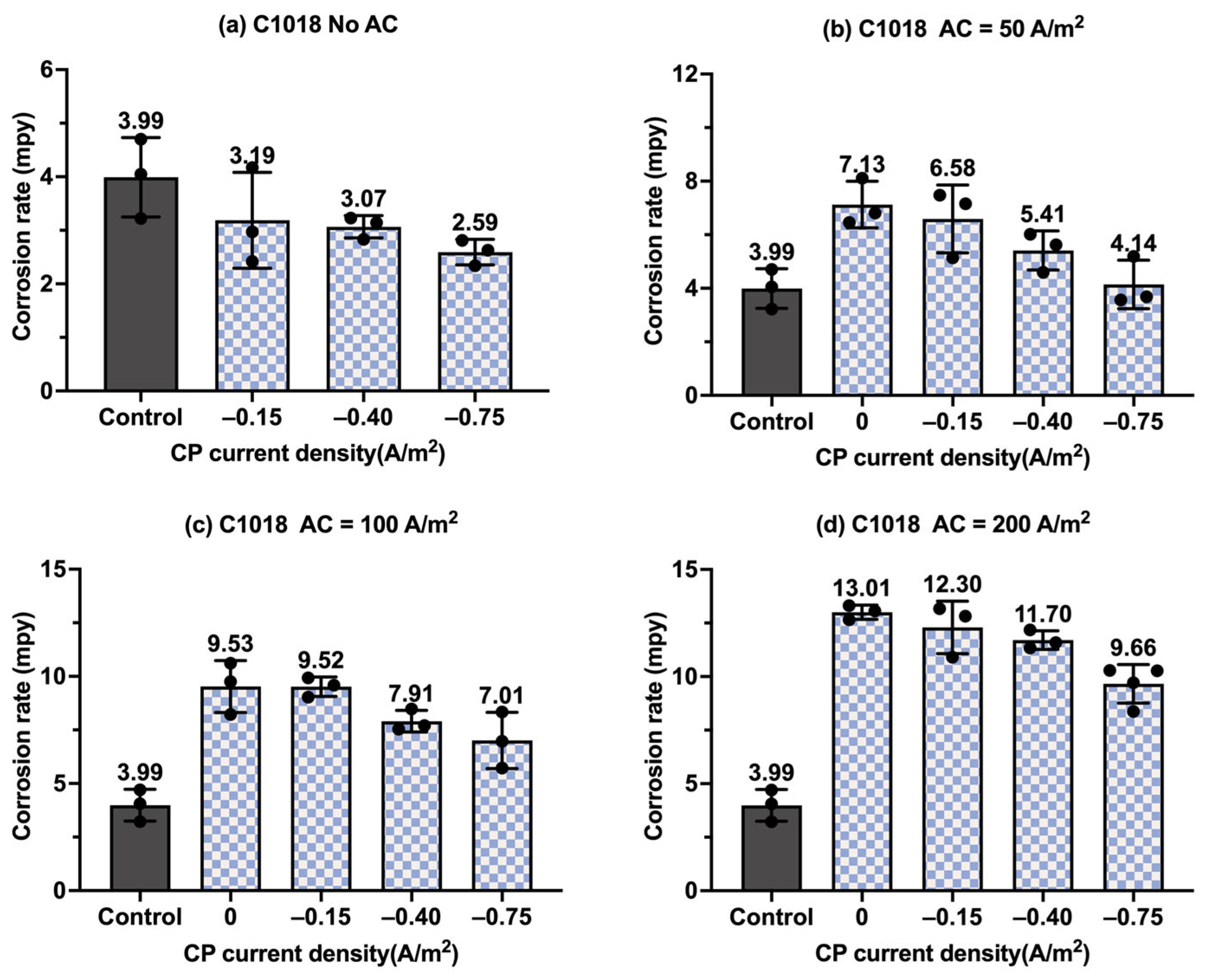
Figure 15.
The corrosion rate of C1018 steel under various AC and CP conditions by Tafel measurements: (a) no AC; (b) AC current density of 50 A/m2; (c) AC current density of 100 A/m2; (d) AC current density of 200 A/m2. The control group is shown in each subfigure to illustrate the natural corrosion rate without AC and CP.
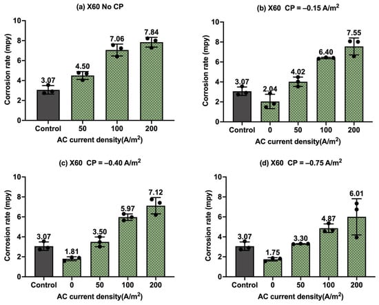
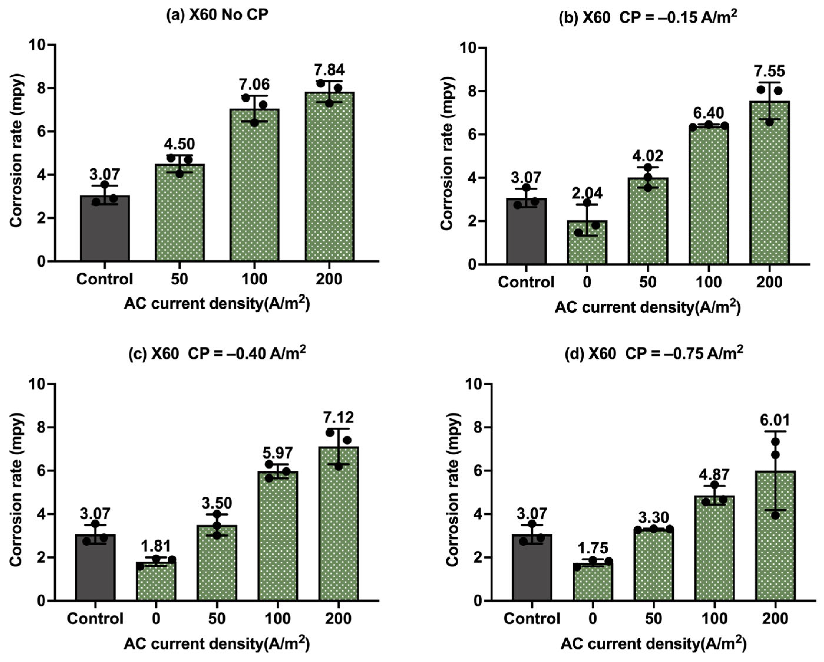
Figure 16.
Corrosion rate of API 5L X60 steel under various AC and CP conditions by Tafel measurements: (a) no CP; (b) CP current density of −0.15 A/m2; (c) CP current density of −0.40 A/m2; (d) CP current density of −0.75 A/m2. The control group is shown in each subfigure to illustrate the natural corrosion rate without AC and CP.
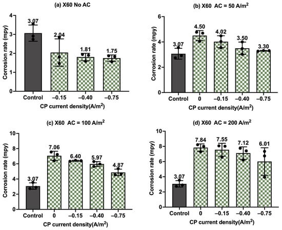
Figure 17.
Corrosion rate of API 5L X60 steel under various AC and CP conditions by Tafel measurements: (a) no AC; (b) AC current density of 50 A/m2; (c) AC current density of 100 A/m2; (d) AC current density of 200 A/m2. The control group is shown in each subfigure to illustrate the natural corrosion rate without AC and CP.
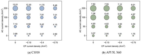
Figure 18.
The corrosion rate of (a) C1018 steel and (b) API 5L X60 under various AC and CP conditions by Tafel measurement. The corrosion rate values are in mpy.
Figure 13a shows the change in the corrosion potential for C1018 steel under different AC and CP current densities. At CP current densities of −0.75 and −0.40 A/m2, as the AC current density increased, the corrosion potential shifted positively to around −0.875 V vs. SCE. In contrast, when CP current density was −0.15 A/m2 or no CP was applied, the corrosion potential shifted more negatively to around −0.855 V vs. SCE. Notably, the corrosion potential exhibited a converging trend as the AC current density rose.
Figure 13b presents the change in the corrosion potential for X60 steel under different AC and CP current densities. At a CP current density of −0.75 A/m2, the corrosion potential shifted positively as the AC current density increased, from −0.905 V vs. SCE to −0.879 V vs. SCE. When CP current density was −0.40 A/m2, the corrosion potential first shifted positively and then shifted negatively, ultimately reaching −0.885 V vs. SCE at 200 A/m2. When CP current density was −0.15 A/m2 or no CP was applied, the corrosion potential shifted more negatively to approximately −0.840 V vs. SCE. This phenomenon indicates that corrosion potential exhibited a converging trend toward around −0.850 V vs. SCE as the AC current density rose to 200 A/m2. This finding is consistent with the trend observed in Figure 13a for C1018 steel and the DC potential shift during the four stages with different CP and AC conditions in Figure 7. Both corrosion potential and DC potential were not effectively affected by CP current density at higher AC interference. It further indicates that the potential change cannot be viewed as the only parameter to determine or evaluate AC corrosion due to its complexity.
Figure 14 shows the corrosion rate of C1018 steel under four AC and CP current densities obtained by Tafel measurements, with the gray columns referring to the control sample under a freely corroding condition, with an average corrosion rate of 3.99 mpy. As shown in Figure 14a, the control sample had a lower corrosion rate than samples under AC interference. Moreover, the corrosion rate increased with the increase in AC current density, signifying that AC interference accelerated the corrosion. However, the corrosion rate values were much lower than the corrosion rate of C1018 obtained from weight loss measurements. Figure 14b–d show the corrosion rate of C1018 steel under cathodic protection with AC interference. When the CP current density was −0.15 A/m2 in Figure 14b, the corrosion rate significantly increased with the introduction of AC current density. This phenomenon thus indicates that this CP level was insufficient for cathodic protection even when the AC current density was 50 A/m2. A similar trend was observed when CP current density was −0.40 A/m2 or −0.75 A/m2.
Figure 15 shows the corrosion rate of C1018 under different CP levels and AC interference when the CP current density is variable in each subplot. Figure 15a shows the corrosion rate of C1018 under different CP current densities when no AC was applied. The corrosion rate decreased with the increase in CP current density, which demonstrates the effectiveness of CP. In Figure 15b, it is evident that when AC current density was 50 A/m2, the three levels of CP current density failed to reduce the corrosion rate. The Tafel data show the inadequacy of CP current density under an AC current density of 50 A/m2. A similar trend was observed at an AC current density of 100 A/m2 (Figure 15c) and 200 A/m2 (Figure 15d).
Similarly to Figure 14, Figure 16 shows the corrosion rate of API 5L X60 steel under different CP and AC current densities by Tafel measurements. The gray columns in each subplot are related to the control sample under a freely corroding condition with 3.07 mpy as the average corrosion rate. Overall, the corrosion rate values were slightly smaller than the corrosion rate of C1018 steel obtained by Tafel measurements, which shows a better corrosion resistance of API 5L X60 compared to C1018 and is consistent with the observation from weight loss measurement in Section 3.3. In addition, the corrosion rate values were smaller than the corrosion rate of API 5L X60 obtained by weight loss measurements.
As shown in Figure 16a, the corrosion rate increased with the introduction of AC current density, and the higher the AC current density, the higher the corrosion rate. This observation again demonstrates that AC interference accelerated steel corrosion. Figure 16b–d illustrate the corrosion rate of API 5L X60 steel under cathodic protection coupled with AC interference. When the CP current density was −0.15 A/m2, as shown in Figure 16b, the corrosion rate was lower than that of the control sample when there was no AC interference. However, the corrosion rate increased considerably with the introduction of AC current density. This phenomenon indicates the insufficiency of cathodic protection when AC interference was introduced. Figure 16c,d present similar results. This observation is in line with that obtained for C1018 steel by Tafel measurements (Figure 15).
Figure 17 presents the corrosion rates of API 5L X60 under different CP and AC levels, enabling the evaluation of the effectiveness of the cathodic protection. Figure 17a shows the corrosion rates of API 5L X60 under cathodic protection without AC interference. It is evident that the corrosion rate decreased as the CP current density increased, indicating enhanced CP effectiveness at higher CP levels. When AC current density was at 50 A/m2 in Figure 17b, the corrosion rate increased compared to the control specimens when no cathodic protection was applied. The corrosion rate decreased with increasing CP; however, even with the CP current density of −0.75 A/m2, the corrosion rate was still larger than that of the control samples. This indicates that the cathodic protection had mitigating effects, but the level of CP used was ultimately not sufficient to fully counteract the corrosion caused by the AC current density of 50 A/m2. Similar observations were observed at AC current density of 100 A/m2 (Figure 17c) and 200 A/m2 (Figure 17d).
Figure 18 shows the average corrosion rate of C1018 and API 5L X60 steel under different CP and AC current densities through bubble charts. As can be seen, higher values of corrosion rate occurred under conditions with higher AC current density and lower CP current density. The corrosion rates from the Tafel measurements indicate that the three levels of cathodic protection were ineffective in slowing the corrosion rate under the AC current densities in this study. However, the corrosion rate under cathodic protection was still lower than that without CP, demonstrating the effectiveness of cathodic protection, particularly when the CP current density was −0.75 A/m2. It decreased the impact of AC interference by 26–42% for C1018 and 23–43% for API 5L X60. Furthermore, the corrosion rate from Tafel measurements was lower than that obtained from weight loss measurements. This might be because the Tafel measurement provides the instantaneous corrosion rate, while the weight loss measurement provides the time-average corrosion rate. Moreover, the sample variations from weight loss measurements were larger than those from Tafel measurements. However, both tests presented the same conclusion that the corrosion rate was accelerated by introducing AC interference and cathodic protection was ineffective at high levels of AC current density.
All in all, the Tafel measurement results show that a higher AC current density accelerated the corrosion rate, and a higher CP current density slowed down the corrosion under the AC and CP conditions in this study. This is consistent with results observed in weight loss experiments in Section 3.3 and DC current from potentiostat mode in Section 3.1. However, the DC potential obtained from galvanostat mode in Section 3.2 did not demonstrate AC-induced corrosion. These findings make us realize that the negative shift in DC potential may not be directly related to the mitigation of corrosion. The DC potential alone may mislead the prediction of AC corrosion, especially at high levels of AC current density.
4. Probabilistic Prediction Model of AC-Induced Corrosion
4.1. Data Review
In this section, a probabilistic model is developed to predict the AC corrosion rate of cathodically protected steels based on experimental data obtained. The experiments resulted in 192 measurements of corrosion growth rate (CR) from the two steel types (i.e., C1018 and X60), four AC current density levels (i.e., 0, 50, 100, 200 A/m2), two CR measurement methods (i.e., Tafel, weight loss (WL)), and four DC current density levels (i.e., 0, −0.15, −0.40, −0.75 A/m2). There are three repetitions for each condition; thus, it resulted in 2 × 4 × 2 × 4 = 64 unique conditions and 64 × 3 = 192 CR measurements.
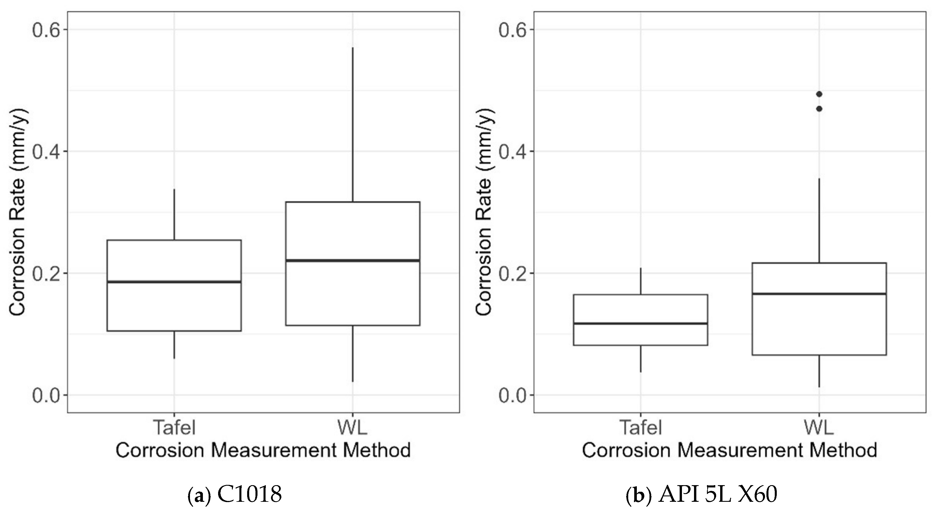
Figure 19 shows the box plots of CR obtained from the two CR measurement methods (i.e., Tafel and WL) and the two types of steel (i.e., C1018 and X60). First, it was observed that overall C1018 steel was more susceptible to AC interference compared to X60 steel, showing generally higher values of CR for C1018 in line with Figure 18. This shows that steel type is an important influencing factor, as expected. In addition, it was found that the WL measurement method led to higher values of CR when compared to the Tafel measurement. This is not surprising, because WL measures mass loss over time; thus, it measures the corrosion rate in an average sense, while Tafel measurement measures the instantaneous corrosion rate. Accordingly, the data obtained from WL and Tafel measurements should be considered separately in model development.
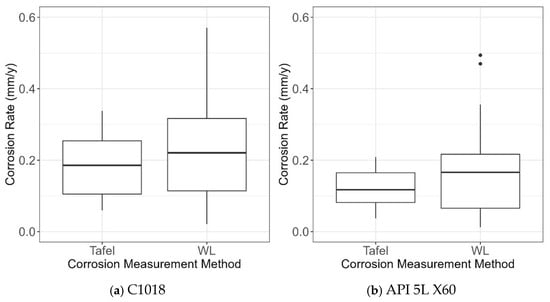
Figure 19.
Box plots of CR data obtained from experimental testing for (a) C1018 and (b) API 5L X60.
4.2. Model Development
Considering corrosion rate is always a non-negative value, a logarithm transformation was used for the CR prediction model, as follows:
where is the point estimate of the corrosion growth rate, σ × ε is the model error, which can be assumed to follow a Normal distribution, N (0, σ) and ε~N (0, 1). In this study, a multi-variable linear regression model was developed for , as follows:
where θ is the vector of unknown model parameters, and x is the independent variable. Ordinary Least Square (OLS) linear regression [38] can be conducted to estimate θ and σ. The considered variables in x can be summarized as mentioned in Table 2.
Table 2.
Considered variables used in probabilistic model development.
It should be noted that the AC/DC variable has been previously [37] shown to be influential on the corrosion rate and thus was considered herein. To ensure the value inside the logarithm function is above zero, AC + 1 and the absolute value of DC were used.
A linear regression model with too many independent variables may face two problems: (1) overfitting that leads to low bias but high variance, and (2) some independent variables may not be statistically significant contributing to the model prediction, making the model formula complicated and application impractical. Thus, a model selection called all-possible-subset model selection was adopted here to select the most important independent variables. In particular, the all-possible-subset examined every possible combination of predictor variables for all model sizes (from one predictor to all predictors), using a criterion, e.g., Adjusted R2, AIC, and BIC, to choose the optimal model. This approach is computationally expensive but ensures that no potentially optimal subset is overlooked [38]. Therefore, after evaluating all possible subsets, the best was selected based on the Adjusted R2, R2adj value [38] and such that all incorporated variables are statistically important. It should be noted that R2adj is a modified version of R2 that has been adjusted for the number of predictors in the model as presented below:
where p is the total number of independent variables in the model, and n is the number of observations. It has to be mentioned that R2 always increases by incorporating more independent variables in the model, thereby reducing the prediction error. However, R2adj does not necessarily increase by increasing the number of independent variables, as shown in Equation (5).
After the model selection, the final developed models based on WL and Tafel experimental results are shown in Equations (6) and (7), respectively:
where the predicted CR values are in mm/y. Table 3 and Table 4 summarize the results of the OLS linear regression analysis. The estimated values for the residuals standard error and model parameters are given along with the associated standard error and p-values.
Table 3.
Statistics of model parameters of the model developed based on CR measured by the WL method.
Table 4.
Statistics of model parameters of the model developed based on the CR measured by the Tafel measurement.
First of all, both models selected the same variables, except that the model based on Tafel measurements did not include DC. Even with one less variable, the model based on Tafel measurements performs better than the model based on WL measurements, since the residuals standard error is less and R2adj is higher for the Tafel model compared to the WL model. Another observation is that when m = 1 (i.e., the metal type is C1018), the logarithm of corrosion rate prediction is increased by a constant value of 0.503 and 0.424 for WL and Tafel, respectively. This is in accordance with the previously shown box plots for the measured corrosion rates, in which the corrosion rate of specimens having steel type C1018 is generally higher than that of X60 steel, for both WL and Tafel measurements. In addition, it is observed that the ratio of AC to DC, represented as log((AC + 1)/|DC|), is statistically significant in both WL and Tafel models, according to p-values being less than 0.05, and hence an influencing factor in corrosion growth.
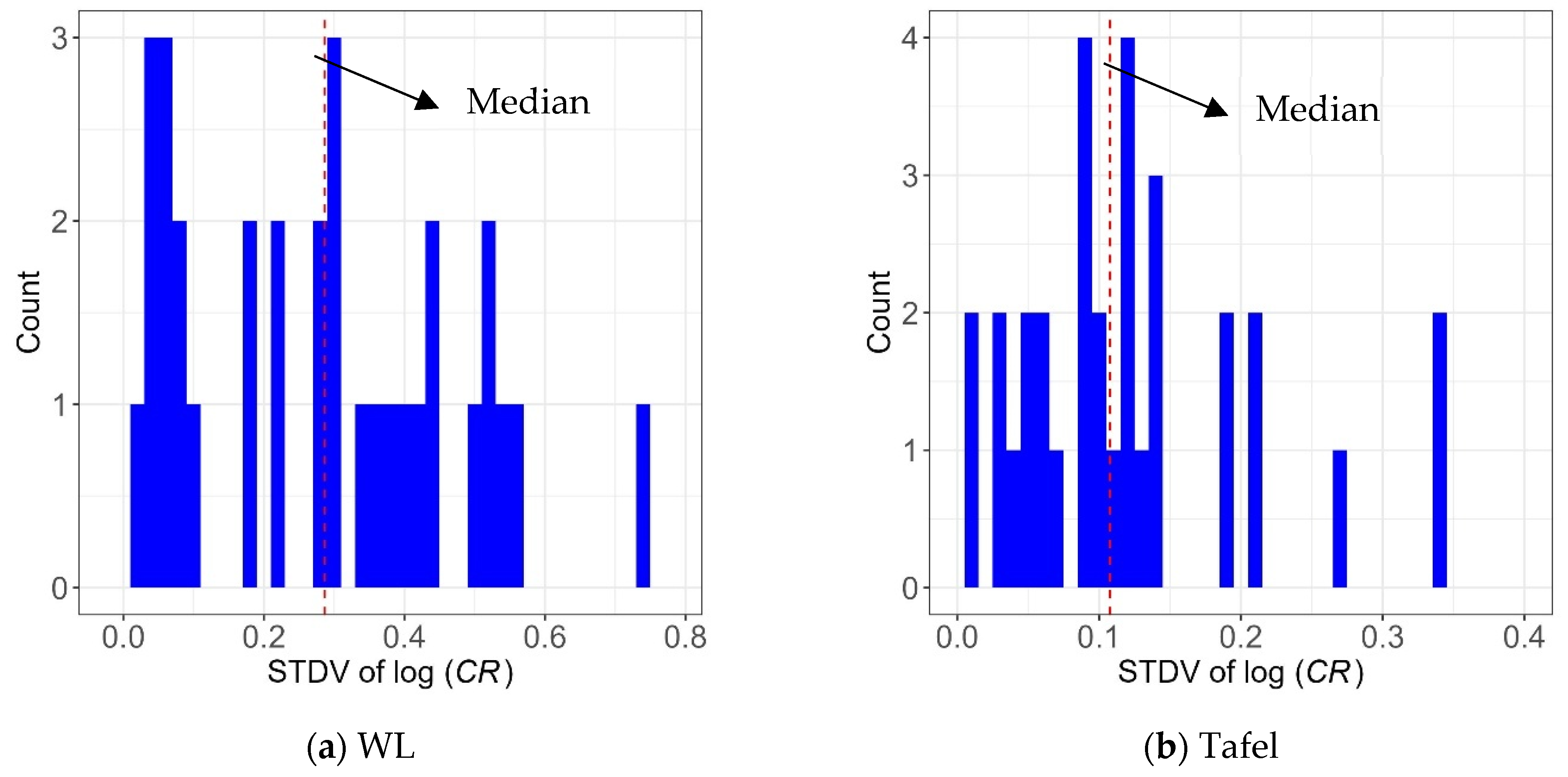
As mentioned earlier, in the dataset used for the model development, the experimental program for model development considered 64 distinct conditions, with three repetitions for each. The repeated experiments resulted in different CR values, as expected, and one could use the sample variance from the repeated experiments to estimate the measurement error. Figure 20 shows the histograms of sample standard deviation (STDV) of the logarithm of CR values obtained using the three repetitions for the two measurement approaches. The median values of the standard deviation of log(CR) are also represented as dashed vertical lines. When comparing Figure 20a,b, they show that the overall standard deviation values are lower for the Tafel measurement compared to the WL method, which indicates less uncertainty in CR values obtained by the Tafel measurement.
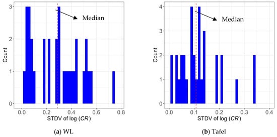
Figure 20.
Histogram of the standard deviation of the logarithm of CR values obtained by three repetitions for (a) WL measurements and (b) Tafel measurements.
In this study, the median value of the sample standard deviation of log(CR) was used as the point estimate of the standard deviation of measurement error, σerror. In this case, σerror = 0.286 and 0.108, respectively, for WL and Tafel measurements. Note that since all the CR values of three repetitions were used in developing the models, the uncertainty in CR values (i.e., the measurement error) was contained in the standard residual errors, σ, obtained by the linear regression analysis. If the measurement error is assumed independent of the model error, the actual variance of the developed model can be calculated by Equation (8):
If the measurement error is assumed to follow a Normal distribution, the model error also follows a Normal distribution. Therefore, the upper and lower bound of a predicted CR value corresponding to an 80% confidence interval can be estimated by Equation (9):
where is the predicted value obtained by the proposed predictive model using Equations (6) and (7).
4.3. Model Performance
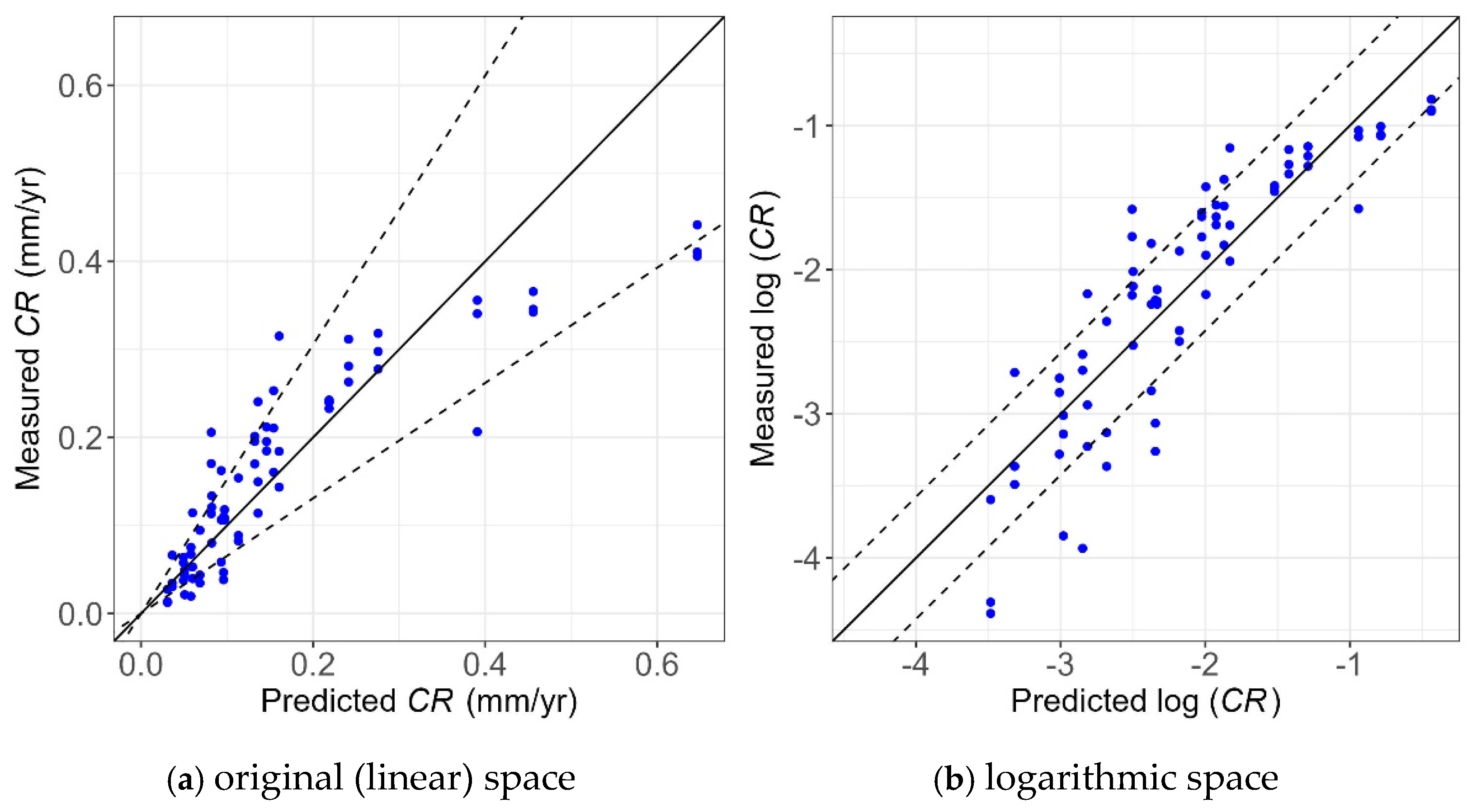
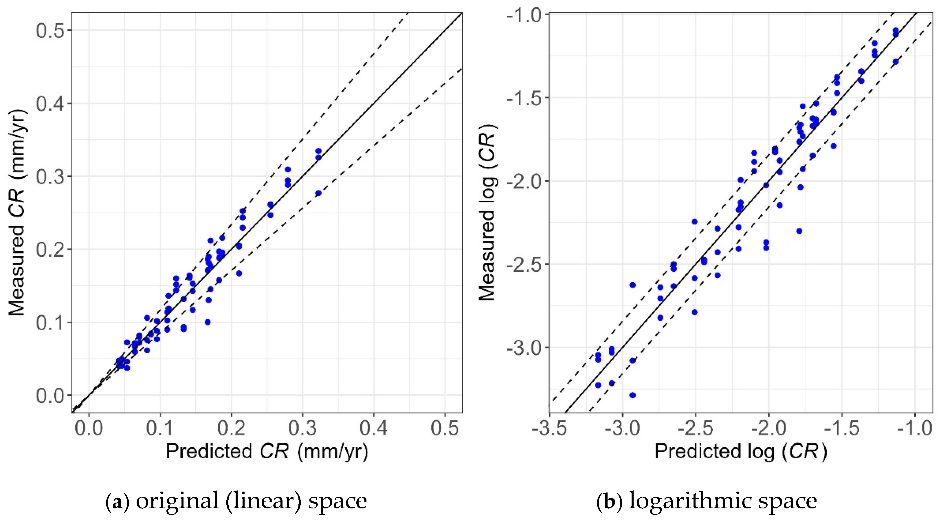
Figure 21 and Figure 22 show the unity plot for the two developed models in the logarithmic and original (linear) spaces, respectively. The unity plot visually shows how well the models are performing. The solid line is the unity line, and the dashed lines correspond to 80% confidence interval considering the corresponding model error (i.e., ) using Equations (8) and (9). Since the logarithm transformation was used, the dashed lines in the original (linear) space diverge with increasing value of CR, as shown in Figure 21.
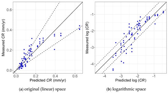
Figure 21.
Unity plot of the WL measurements vs. WL prediction model in the (a) original (linear) and (b) logarithmic spaces.
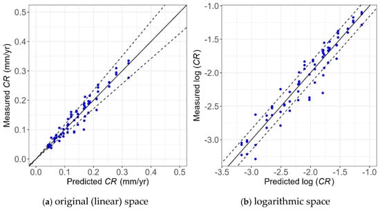
Figure 22.
Unity plot of the Tafel measurements and Tafel prediction model in the (a) original (linear) and (b) logarithmic spaces.
As shown, most of the points lie within the 80% confidence interval, showing the high accuracy of the models. In addition, these points are evenly scattered around the unity line, showing the model provides unbiased predictions of experimental values. Also, the narrower bounds shown in Figure 22a compared to Figure 21a indicate the model using the Tafel measurement has less uncertainty than the one using WL measurements, which is consistent with the findings obtained from Table 3 and Table 4.
4.4. Sensitivity Analysis
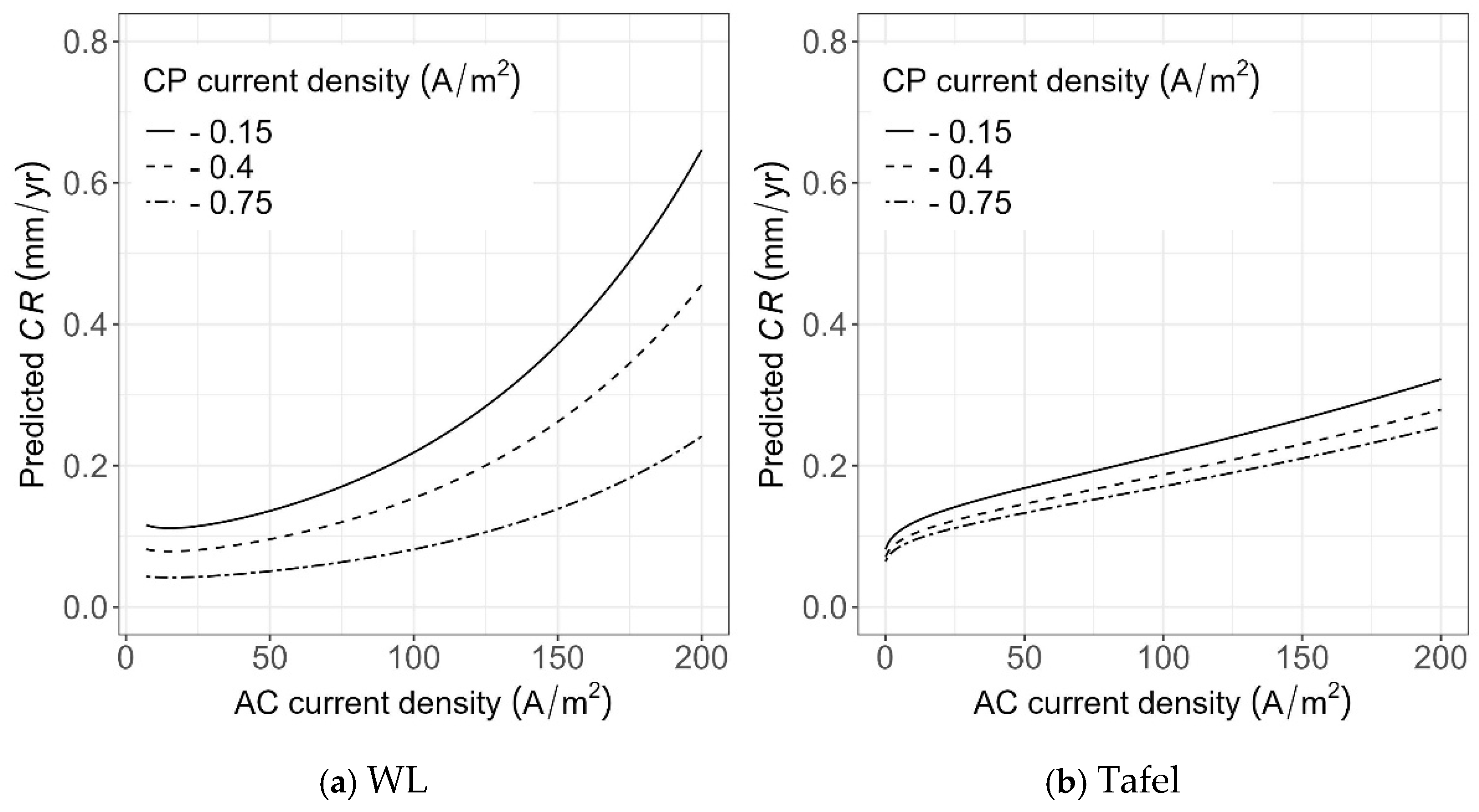
Considering that the induced AC current density on a pipeline can fluctuate over time, it is essential to understand how AC current density impacts the CR, given a certain level of CP current density. In this section, the sensitivity of CR to the values of AC under three different CP levels (in terms of CP current density) was evaluated. In particular, the C1018 steel type was used as an example, while AC current density varied from 10 to 200 A/m2, and the CP current densities were −0.15, −0.40, and −0.75 A/m2.
As shown in Figure 23, given a CP level, the CR increases with increasing AC current density. However, the prediction using the model based on WL measurement (as shown in Figure 23a) is more sensitive to either AC current densities or CP levels, and the slope of CR increases with AC current density. Such increases are more apparent when the CP current density is low (e.g., CP density of −0.15 A/m2). In addition, the CR values obtained from the model based on the WL measurements are considerably higher compared to those from the Tafel measurements for low values of CP density (e.g., CP density of −0.15 A/m2); however, for CP density of −0.75 A/m2, the predicted CR values based on the two models are similar.

Figure 23.
Sensitivity of CR predictions to AC and DC current densities using the developed models based on (a) WL measurements and (b) Tafel measurements.
5. Conclusions
In this research, real-time electrochemical measurements and corrosion rate analysis were performed on pipeline steel in a simulated soil solution under cathodic protection and AC interference. This enabled a comprehensive evaluation of the effect of AC and CP on pipeline steel, providing a more precise understanding of the corrosion behavior of the pipeline. Based on the experimental results, two probabilistic models were developed to predict the corrosion rate of steel with high accuracy, according to the two utilized measurement methods, i.e., weight loss (WL) or Tafel measurement. The uncertainty in the measurements was also considered during the model development.
It was found that the presence of AC interference caused a shift in the DC potential or DC current density away from the designed CP values. The DC current density shifted to an obvious anodic current density with the application of AC interference, indicating the occurrence of corrosion. Additionally, the DC current density shifted to the cathodic part when the AC current density was low and the applied CP potential was more negative than the conventional standard, indicating that the metal was protected. However, the DC potential shifted more negatively than the open circuit potential when AC was applied to the steel, no matter whether CP was applied or not. This DC potential change misleads AC-induced corrosion, which cannot be used alone to study AC corrosion.
It was found that the corrosion rate of C1018 and API 5L X60 steel increased with the presence of AC interference and decreased with more negative CP levels. Also, for the same AC and CP conditions, overall, C1018 steel is more susceptible to AC interference compared to X60 steel. However, even with CP current densities, the corrosion rates may still exceed the natural corrosion rate for carbon steel in certain scenarios. It was shown that the corrosion rate and its variability measured by the Tafel measurement was lower than the rate and the variability from the WL method. The final formulations for both developed prediction models showed the importance of ratios of AC and DC current densities on the corrosion rate, consistent with the findings from previous studies. The developed models would be particularly useful to predict corrosion over time to estimate corrosion risk, particularly when AC fluctuates over time, which is common in reality.
Supplementary Materials
The following supporting information can be downloaded at: https://www.mdpi.com/article/10.3390/cmd6020026/s1, The supporting materials include the morphology of API 5L X60 and C1018 after weight loss measurements and the kinetic parameters derived from Tafel plots for both metals. Figure S1: The morphology of (a) API 5L X60 and (b) C1018 after the weight loss measurement, followed by the cleaning procedure of ASTM G-1.; Table S1: Kinetic parameters derived from Tafel plots for C1018 steel immersion in simulated soil solution at 25℃ under various AC and CP conditions; Table S2: Kinetic parameters derived from Tafel plots for API 5L X60 steel immersion in simulated soil solution at 25℃ under various AC and CP conditions.
Author Contributions
Y.S.: methodology, data curation, investigation, formal analysis, original draft preparation; E.M.F.: methodology, data curation, investigation, formal analysis, original draft preparation; Q.H.: concept, supervision, methodology, writing—review and editing; Q.Z.: concept, supervision, methodology, writing—review and editing. All authors have read and agreed to the published version of the manuscript.
Funding
USDOT PHMSA Competitive Academic Agreement Program (CAAP), contract number 693JK32050008CAAP.
Data Availability Statement
Data will be made available on request.
Acknowledgments
The authors thank Tanner Laughorn, Abigail Murray, and Abigail Acurio for their assistance in lab work. This research was supported by the U.S. Department of Transportation Pipeline and Hazardous Materials Safety Administration (PHMSA, contract number 693JK32050008CAAP).
Conflicts of Interest
The authors declare no conflicts of interest.
References
- Cheng, Y.F. AC Corrosion of Piplelines; Ampp: Houston, TX, USA, 2021; ISBN 978-1-57590-400-9. [Google Scholar]
- Xu, L.Y.; Su, X.; Caheng, Y.F. Effect of Alternating Current on Cathodic Protection on Pipelines. Corros. Sci. 2013, 66, 263–268. [Google Scholar] [CrossRef]
- Kuang, D.; Cheng, Y.F. AC Corrosion at Coating Defect on Pipelines. Corrosion 2015, 71, 267–276. [Google Scholar] [CrossRef] [PubMed]
- Palumbo, G.; Górny, M.; Banaś, J. Corrosion Inhibition of Pipeline Carbon Steel (N80) in CO2-Saturated Chloride (0.5 M of KCl) Solution Using Gum Arabic as a Possible Environmentally Friendly Corrosion Inhibitor for Shale Gas Industry. J. Mater. Eng. Perform. 2019, 28, 6458–6470. [Google Scholar] [CrossRef]
- Davoodi, F.; Akbari-Kharaji, E.; Danaee, I.; Zaarei, D.; Shishesaz, M. Corrosion Behavior of Epoxy/Polysulfide Coatings Incorporated with Nano-CeO2 Particles on Low Carbon Steel Substrate. Corrosion 2022, 78, 785–798. [Google Scholar] [CrossRef]
- Yunovich, M.; Thompson, N.G. AC Corrosion: Corrosion Rate and Mitigation Requirements; OnePetro: Richardson, TX, USA, 2004. [Google Scholar]
- Gummow, R.A.; Wakelin, R.G.; Segall, S.M. AC Corrosion: A New Threat to Pipeline Integrity? In Proceedings of the 1996 1st International Pipeline Conference, Calgary, AB, Canada, 9–13 June 1996; Volume 1: Regulations, Codes, and Standards; Current Issues; Materials; Corrosion and Integrity; American Society of Mechanical Engineers. pp. 443–453. [Google Scholar]
- Wang, H.; Du, C.; Liu, Z.; Wang, L.; Ding, D. Effect of Alternating Current on the Cathodic Protection and Interface Structure of X80 Steel. Materials 2017, 10, 851. [Google Scholar] [CrossRef]
- Xu, L.Y.; Su, X.; Yin, Z.X.; Tang, Y.H.; Cheng, Y.F. Development of a Real-Time AC/DC Data Acquisition Technique for Studies of AC Corrosion of Pipelines. Corros. Sci. 2012, 61, 215–223. [Google Scholar] [CrossRef]
- Tang, D.Z.; Du, Y.X.; Lu, M.X.; Jiang, Z.T.; Dong, L.; Wang, J.J. Effect of AC Current on Corrosion Behavior of Cathodically Protected Q235 Steel: AC Corrosion of Cathodically Protected Q235 Steel. Mater. Corros. 2013, 66, 278–285. [Google Scholar] [CrossRef]
- Kuang, D.; Cheng, Y.F. Effects of Alternating Current Interference on Cathodic Protection Potential and Its Effectiveness for Corrosion Protection of Pipelines. Corros. Eng. Sci. Technol. 2016, 52, 22–28. [Google Scholar] [CrossRef]
- Ormellese, M.; Goidanich, S.; Lazzari, L. Effect of AC Interference on Cathodic Protection Monitoring. Corros. Eng. Sci. Technol. 2011, 46, 618–623. [Google Scholar] [CrossRef]
- SP0169-2013; Control of External Corrosion on Underground or Submerged Metallic Piping Systems. NACE: Houston, TX, USA, 2013.
- Edward, M. Introduction to Corrosion Science; John Wiley & Sons: Hoboken, NJ, USA, 2008; ISBN 978-0-470-27725-6. [Google Scholar]
- Du, Y.; Tang, D.; Lu, M.; Chen, S. Researches on the Effects of AC Interference on CP Parameters and AC Corrosion Risk Assessment for Cathodic Protected Carbon Steel. In Proceedings of the CORROSION 2017, New Orleans, LA, USA, 26–30 March 2017; OnePetro: Richardson, TX, USA, 2017. [Google Scholar]
- Ormellese, M.; Lazzari, L.; Brenna, A.; Trombetta, A. Proposal of CP Criterion in the Presence of AC-Interference. In Proceedings of the NACE CORROSION, San Antonio, TX, USA, 14–18 March 2010; p. 18. [Google Scholar]
- Brenna, A.; Lazzari, L.; Pedeferri, M.; Ormellese, M. Cathodic Protection Condition in the Presence of AC Interference. Corrosione 2014, 6, 29–34. [Google Scholar]
- Tang, D.; Du, Y.; Li, X.; Liang, Y.; Lu, M. Effect of Alternating Current on the Performance of Magnesium Sacrificial Anode. Mater. Des. 2016, 93, 133–145. [Google Scholar] [CrossRef]
- Ormellese, M.; Lazzari, L.; Brenna, A. AC Corrosion of Cathodically Protected Buried Pipelines: Critical Interference Values and Protection Criteria. In Proceedings of the NACE—International Corrosion Conference Series, Dallas, TX, USA, 15–19 March 2015; Volume 2015. [Google Scholar]
- He, X.; Jiang, G.; Qiu, Y.; Zhang, G.; Jin, X.; Xiang, Z.; Zhang, Z.; Tang, H. Study of Criterion for Assuring the Effectiveness of Cathodic Protection of Buried Steel Pipelines Being Interfered with Alternative Current. Mater. Corros. 2011, 63, 534–543. [Google Scholar] [CrossRef]
- Olesen, A.J.; Dideriksen, K.; Nielsen, L.V.; Møller, P. Corrosion Rate Measurement and Oxide Investigation of AC Corrosion at Varying AC/DC Current Densities. Corrosion 2019, 75, 1026–1033. [Google Scholar] [CrossRef]
- Guo, Y.-B.; Liu, C.; Wang, D.-G.; Liu, S.-H. Effects of Alternating Current Interference on Corrosion of X60 Pipeline Steel. Pet. Sci. 2015, 12, 316–324. [Google Scholar] [CrossRef]
- Moran, A.; Lillard, R.S. AC Corrosion Evaluation of Cathodically Protected Pipeline Steel. Corrosion 2019, 75, 144–146. [Google Scholar] [CrossRef]
- Goidanich, S.; Lazzari, L.; Ormellese, M. AC Corrosion. Part 2: Parameters Influencing Corrosion Rate. Corros. Sci. 2010, 52, 916–922. [Google Scholar] [CrossRef]
- Fu, A.Q.; Cheng, Y.F. Effect of Alternating Current on Corrosion and Effectiveness of Cathodic Protection of Pipelines. Can. Metall. Q. 2012, 51, 81–90. [Google Scholar] [CrossRef]
- Xiao, Y.; Du, Y.; Tang, D.; Ou, L.; Sun, H.; Lu, Y. Study on the Influence of Environmental Factors on AC Corrosion Behavior and Its Mechanism. Mater. Corros. 2018, 69, 601–613. [Google Scholar] [CrossRef]
- Guo, Y.; Meng, T.; Wang, D.; Tan, H.; He, R. Experimental Research on the Corrosion of X Series Pipeline Steels under Alternating Current Interference. Eng. Fail. Anal. 2017, 78, 87–98. [Google Scholar] [CrossRef]
- Qin, Q.; Wei, B.; Bai, Y.; Fu, Q.; Xu, J.; Sun, C.; Wang, C.; Wang, Z. Effect of Alternating Current Frequency on Corrosion Behavior of X80 Pipeline Steel in Coastal Saline Soil. Eng. Fail. Anal. 2021, 120, 105065. [Google Scholar] [CrossRef]
- Thakur, A.K.; Arya, A.K.; Sharma, P. Analysis of Cathodically Protected Steel Pipeline Corrosion under the Influence of Alternating Current. Mater. Today Proc. 2022, 50, 789–796. [Google Scholar] [CrossRef]
- Zhu, M. Corrosion Behavior of X65 and X80 Pipeline Steels under AC Interference Condition in High pH Solution. Int. J. Electrochem. Sci. 2018, 13, 10669–10678. [Google Scholar] [CrossRef]
- Wang, L.; Cheng, L.; Li, J.; Zhu, Z.; Bai, S.; Cui, Z. Combined Effect of Alternating Current Interference and Cathodic Protection on Pitting Corrosion and Stress Corrosion Cracking Behavior of X70 Pipeline Steel in Near-Neutral pH Environment. Materials 2018, 11, 465. [Google Scholar] [CrossRef] [PubMed]
- Wang, X. Study on Corrosion and Delamination Behavior of X70 Steel under the Coupling Action of AC-DC Interference and Stress. Int. J. Electrochem. Sci. 2019, 1968–1985. [Google Scholar] [CrossRef]
- Yang, J.; Le, Z.; Zhao, B.; Ma, J.; Yuan, Y. Influence of Alternating Current on Corrosion Behavior of X100 Steel in Golmud Soil Simulated Solution with Different pH. Int. J. Electrochem. Sci. 2020, 15, 10423–10431. [Google Scholar] [CrossRef]
- Xu, L.; Shi, S.; Huang, Y.; Yan, F.; Yang, X.; Bao, Y. Corrosion Monitoring and Assessment of Steel under Impact Loads Using Discrete and Distributed Fiber Optic Sensors. Opt. Laser Technol. 2024, 174, 110553. [Google Scholar] [CrossRef]
- Xu, L.; Shi, S.; Yan, F.; Huang, Y.; Bao, Y. Experimental Study on Combined Effect of Mechanical Loads and Corrosion Using Tube-Packaged Long-Gauge Fiber Bragg Grating Sensors. Struct. Health Monit. 2023, 22, 3985–4004. [Google Scholar] [CrossRef]
- Ahmad, Z. Principles of Corrosion Engineering and Corrosion Control; Elsevier: Amsterdam, The Netherlands, 2006; ISBN 978-0-08-048033-6. [Google Scholar]
- Farahani, E.M.; Su, Y.; Chen, X.; Wang, H.; Laughorn, T.R.; Onesto, F.; Zhou, Q.; Huang, Q. AC Corrosion of Steel Pipeline under Cathodic Protection: A State-of-the-art Review. Mater. Corros. 2023, 75, 290–314. [Google Scholar] [CrossRef]
- James, G. An Introduction to Statistical Learning: With Applications in R, 1st ed.; Springer: New York, NY, USA, 2013; ISBN 978-1-4614-7137-0. [Google Scholar]


Disclaimer/Publisher’s Note: The statements, opinions and data contained in all publications are solely those of the individual author(s) and contributor(s) and not of MDPI and/or the editor(s). MDPI and/or the editor(s) disclaim responsibility for any injury to people or property resulting from any ideas, methods, instructions or products referred to in the content. |
© 2025 by the authors. Licensee MDPI, Basel, Switzerland. This article is an open access article distributed under the terms and conditions of the Creative Commons Attribution (CC BY) license (https://creativecommons.org/licenses/by/4.0/).