Magnetic Force-Free Theory: Nonlinear Case


1
Department of Physics, University La Sapienza, 00185 Rome, Italy
2
Centro Ricerche Enea, Frascati, Via Enrico Fermi, Frascati, 00044 Rome, Italy
*
Author to whom correspondence should be addressed.
Physics 2022, 4(1), 21-36; https://doi.org/10.3390/physics4010003
Submission received: 21 June 2021
/
Revised: 15 October 2021
/
Accepted: 18 November 2021
/
Published: 10 January 2022
(This article belongs to the Section Statistical Physics and Nonlinear Phenomena)
Abstract
:In this paper, a theory of force-free magnetic field useful for explaining the formation of convex closed sets, bounded by a magnetic separatrix in the plasma, is developed. This question is not new and has been addressed by many authors. Force-free magnetic fields appear in many laboratory and astrophysical plasmas. These fields are defined by the solution of the problem with some field conditions on the boundary of the plasma region. In many physical situations, it has been noticed that is not constant but may vary in the domain giving rise to many different interesting physical situations. We set with being the poloidal magnetic flux function. Then, an analytic method, based on a first-order expansion of with respect to a small parameter , is developed. The Grad–Shafranov equation for is solved by expanding the solution in the eigenfunctions of the zero-order operator. An analytic expression for the solution is obtained deriving results on the transition through resonances, the amplification with respect to the gun inflow. Thus, the formation of spheromaks or protosphera structure of the plasma is determined in the case of nonconstant .
1. Introduction
Force-free magnetic field are important for plasma physics in various magnetically dominated environments, like spheromaks in the laboratory and relativistic jets in astrophysical plasma. Relaxed magnetohydrodynamic (MHD) states with negligible pressure gradient contribution negligible to the force balance were introduced by Taylor in 1974 [1] (see also [2]). Taylor postulated that they are minimum of the magnetic energy and arise as a consequence of a self-organization of the magnetic field . The defining property is , with a constant for all the plasma region V. This equation is derived by minimizing the magnetic energy (where is the magnetic permeability of free space) in a volume V (r is the radius) subject to the constraint of conservation of the helicity and that the vector potential is orthogonal to the boundary , i.e., on the boundary , such a state is called Taylor state. The theory of Jensen and Chu [3] predicts conditions for accessing the Taylor states, the eigenvalues of the above equation being barriers. There is experimental evidence that a magnetized plasma inside a conducting boundary will spontaneously reach a configuration near a Taylor state [4]. In [3], a mechanism of electrostatic helicity injection is described. This is done by providing conducting limiters with electric gaps that divide limiters into sections for which magnetic field lines enter and leave the limiter. When these sections are electrically connected to a terminals of a DC (direct current) power supply, electrostatic helicity injection may be accomplished, thus allowing DC drive of toroidal configurations. On much larger scale of kilo-to-mega parsec are the self-organized magnetic bubbles generated by an accretions disk of a black hole of a billion stellar mass [5,6], or the magnetic field in the Sun photosphere [7,8]. According to the theory of Jensen and Chu, the force-free magnetic relaxation takes place for smaller than the smallest eigenvalue of the problem , , on the boundary of the volume. More complicated force-free solutions such as flipped spheromak and multiple internal magnetic islands were not accessible. However, the situation is more complex because some situations not forecasted by the theory of Jensen and Chu take place. In the actual driven plasma the factor may change in the domain and then other energetic configurations can appear. This has been noticed in [9]. There, it is reported that in a compact toroid experiment (CTX) which give spheromaks equilibria (determined in a non perturbing manner) is not constant. The departure in magnetic energy of these equilibria with respect to the minimum-energy state is small. Coherent oscillations are seen, generated by rotating kink modes within equilibria. The onset of the modes is shown to be consistent with the slope of from the equilibrium measurement. If the scalar depends weakly on the poloidal flux then a broad range of force-free solutions can become accessible like the flipped spheromak described by Rosenbluth and Bussac [10], a configuration of the plasma being a toroid bounded by a magnetic separatrix. Such a configuration is in agreement with the results of Tang and Boozer [11]. In such a situation, it is interesting to study the neighbors of the Taylor state with weakly depending on . Such a study has been already done in [11] using numerical methods.
In current paper, an analytic theory, based on a perturbation method, is developed to investigate some other cases of Taylor states, a magnet in the upper half of the spheromak is introduced, the effect on the formation of the plasma structure and the influence on the resonance condition are studied, the resonance being responsible for the formation of the closed convex level curves of . An explicit model for the magnet [12] is considered in this paper as well as a model for the gun [13], the gun is a stationary inflow of magnetic field. There are results using the gun also in [14]. Since we find an analytic solution, it is easier to study the dependence of the solutions on the boundary conditions.
This paper is organized as follows. In Section 2, the nonlinear dependence of on the flow function is introduced, and to a small parameter is given; then, the problem with magnet condition on the boundary is solved and the corresponding graphs are plotted. In Section 3, the problem without the magnet condition is solved showing the possibility of having the spheromak [13] or protosphera [15,16] condition. Section 4 gives the conclusions.
2. Nonlinear Grad–Shafranov Equation
2.1. Nonlinear
In order to obtain the condition of the spheromak or protosphera existence, one needs to find the level curves of the poloidal flow function . Thus, one needs to find the properties of the solutions of the Grad–Shafranov (G-S) Equation [17,18],
where I and are axisymmetric functions depending on . is a poloidal flow through a circle of radius r at axial location z, and I is a poloidal current.
In what follows, we analyze an axisymmetric plasma and introduce a nonlinear dependence of on . The nonconstant values of were observed in many different plasmas. We start with the smallest power dependence on higher than 1 and choose a quadratic dependence since the states corresponding to a linear one can be stable but can also decay [11]. A normalization value for the flow function is used, i.e., let be the maximal flux; then, condition is chosen being similar to the one introduced in [13],
The nonlinear dependence on is introduced by means of a small parameter . The maximal flux must be introduced in order to have the spatial excursion of of the order of . We introduce a small nonlinear dependence on of the order of . This choice of satisfies the normalization condition,
This kind of normalization does not fix the value of . Since we are going to expand our solution in the parameter , the parameter has to be small enough with respect to the maximal flow , thus we are free to make the optimal choice. The expression for the poloidal current I is derived from
Then,
so that
where the terms of the order are neglected.
2.2. First-Order Perturbation in
Now, let us settle the perturbation method for computing analytically the solution of the G-S equation with the nonlinear .
Define the operator D as
Then one has to solve the G-S equation dropping the term:
Then, scaling the by using the first-order expansion,
and taking only the zero-order and first-order terms of Equation (8),
and separating the term of different orders in , one obtains the system
The calculations in this paper are done in axis symmetric situation in a cylinder of the height h and the radius a, with a “gun” magnetic flux injection at [13]. satisfies the non-homogenous boundary conditions (b.c.) defined in the next Section. satisfies the non-homogeneous equation with zero b.c.
In this way, can be found by expanding it in eigenfunctions of the equation of the zero-order operator with zero b.c. conditions at the boundary of the cylinder, . These eigenfunctions can be found using the variable separation, :
which can be separated into the two equations:
where m is an arbitrary integer.
Then , define
The equation for can be solved choosing and using the identity,
The b.c. in a can be satisfied if one sets , where is the n-th root of the Bessel function . Thus, the eigenfunctions of the zero-order operator are:
and
Here, are set and are the eigenvalues of the homogenous problem, which is used below to obtain the equation for .
2.3. Solution of Zero-Order Equation and Boundary Conditions
In order to have a realistic model for the protosphera, one needs to choose realistic non-homogenous boundary conditions. Below, a cylinder of radius and height are considered. At the boundary , a magnet is inserted which generates a magnetic field of the form [12]:
Since the solutions of the problem under study can be found expanding in Bessel functions, it is more suitable the boundary condition on is given in terms of the Bessel functions. Then, one can approximate the expression of with the Bessel function :
Let us choose . is the second root of , the Bessel function of zero order. The behaviour of of Equations (18) and (19) are quite similar, as shown in Figure 1.
Then, the following boundary conditions are chosen:
Here, is the magnetic field created by an external coil which penetrates at the gas end wall, is the Heaviside theta function.
Let us remark here that there is a general theorem shown by Solov’ev and Kirichek [19] such that a necessary condition to have a force-free Taylor field with nonconstant is to have an applied longitudinal external field . Then, the b.c. (20) at is a necessary condition for having a force-free Taylor state with a nonconstant .
We apply the general theory of the force-free magnetic field to solve the equation for . One needs to find the expression of which is at the right-hand side of Equation (11) for . The general force-free equation together with the b.c. for to solve is
The solution of this equation to be used for getting . However, using the nonlinear expression of , defined here, introduces terms of the higher-order s. So, one finds the solution of the linearized equation,
From the general theory of force-free field [13], one knows that the solution of this equation has the form
where is the unit vector on the z-axis, and is a scalar function satisfying the Helmholtz equation,
From this theory, one obtains:
Let
then,
where is generated from the separation of variables of the problem. Choosing , one finds the solution
This choice allows us to obtain the solution for the magnetic field which satisfies the boundary conditions. In fact, the components of the magnetic field are obtained using the identity :
From these expressions, it follows that because , being the theta function. concides within a good approximation with the b.c. (19) as soon as one chooses , thus another condition for is obtained:
We find that the choice of for fixes the value of from the solution (28) for , so the incoming flux from the gun is not arbitrary:
Thus:
The flow function is found in the following way. The most general is given by
where . Using , one gets:
From this:
2.4. Solution of the First-Order Equation
Let us study the solution of the first-order equation,
is expanded in eigenfunctions of the zero-order equation:
where are the roots of . The functions are normalized with the norm of the eigenfunctions, :
So, the orthogonality of the Bessel function is given by
The sine functions are also normalized:
Inserting in the equation for , one gets:
Multiplying both sides of this equation by and by and then integrating, one finds:
where the constants are:
The integrals over z give:
The integrals over r are computed numerically.
The values of , and , computed for , are shown in Table 1 for .
In Table 2, the first six values of and are shown.
The results are summarized as follows:
The singularities in the denominator of the function in Equation (44) are not new as were already found in [3] and confirmed by the results of [11]. The singularities generate the energy barriers between different Taylor states having different properties. A diverging behaviour as approaches the first eigenvalue implies flux amplification that is desired in any dynamo theory. The Taylor state in [11] around the primary resonance is that of spheromak magnetic topology. The state after the first resonance is the flipped spheromak obtained in [11], a single connected toroid bounded by a magnetic separatrix, also described by Rosenbluth and Bussac [10].
Figure 2 shows the contour plot of , and Figure 3 shows the contour plot of for , , and . In the following Sections, the dependence on the parameter is explored for different models that allow free choices of by dropping the boundary conditions due to the magnet.
Interestingly, the contour lines, created by the boundary condition on the magnet, tend to remain concentrated in the left part of the figure with increasing . The perturbed field shows localized closed convex field lines typical of the plasma. So, the boundary condition on the magnetic field support the plasma structure of the spheromak or the protosphera. The model has too many contraints: the magnet condition is a constraint also for the gun inflow and there is no free choice for values because the condition on imposes , so that, with this model, one cannot study the resonances due to the zero of the denominators in ; see Equation (44). It has been already shown that can pass through these resonances [11,14]. Thus, the model without magnet, discussed in the next Section, is of higher interest because one can study the transitions through the singularities and how they depend on . In this model, one can study the stability of the solution with respect to the variation of . The graphs are plotted for are shown in Figure 4. With the increase of , the fluctuations of increase; for values larger than , the graphs demonstrate instability of the solution.
3. Taylor States without the Magnet
Let us drop the magnet condition and use other boundary conditions. is not given by the assigned magnetic field but is equal to free solution of the problem:
Solving the equation for ,
and using the variable separation, one obtains:
where . Choosing , the solution is with a free parameter:
This choice allows us to obtain the solution for the magnetic field which satisfies the boundary conditions. In fact, the components of the magnetic field are obtained using the identity :
Thus, in this theory, one again obtains that the incoming flow of the gun is constrained by the solution.
However, in this case, there is no constraint on , so the parameter is free and one can investigate the resonances. The solution is found using :
Inserting this expression in the equation for , one obtains:
With but with kept a free parameter one can study the transition through the resonances.
First, the case is studied with the resonance at . Figure 5 shows and the level curves of for and . From this graph, similar to the case of the magnet, the value is used because the perturbation is too large with respect to the perturbed term .
Having found the value of which gives a meaningful result one can study the resonance. Clearly, this value of is valid both for the resonance at and at . First, in Figure 6, the poloidal flux function around the first resonance is plotted for chosen.
We remark here that there is a symmetry around for and ; there are negative minima above the line and positive minima below this line. For higher values of , the situation becomes reverse .This could be a signature of an instability of the solution. This instability can be caused also by the b.c. chosen in this particular example. Of course, one would need to study this solution for other b.c. Moreover, the numerical values are seen to be antisymmetric with respect to . The level curves are approximately ellypses and also the form of the ellypses are symmetric. It is not straight to justify the form of the level curves, but the origin can be understood as follows. The Bessel function has a simple form in the interval , and the trigonometric function obeys oscillations in z. Interestingly, the two functions combine giving rise to the typical closed lines in spheromaks. It is remarkable that there is a sudden growth of the level curves for indicating an existence of a resonance; the theoretical resonance exists for but there are numerical errors which influence the result. In addition, one has to remark that this instability may cause problems in the numerical evaluation of the magnetic energy; therefore, it is preferrable to study the level curves. The analytic expressions obtained here have the advantage of making it relatively easier the study of the effects of changing the b.c. The curves in Figure 6 are typical closed curves of the flipped spheromaks, already observed by Rosenbluth and Bussac [10], which represents a single connected toroid, bounded by a magnetic separatrix. As so, then, there is the formation of a configuration of spheromak or protosphera. Such resonances, already obtained by Tang and Boozer [11], coincide with those obtained by Jensen and Chu [3]. In [11], one can find the peaks in magnetic energy located at the eigenvalues of the force-free G-S equation, derived for a certain representation of the magnetic field .
The current study considers a different starting representation, the one in [13], the corresponding eigenvalues are those obtained by different procedures for solving a different partial differential equations. The other difference is that the b.c. for the magnetic field are not introduced in [11], while here two different cases are explicitly treated, one with the magnet and the other one without. In the first case, it is shown that there are no resonances, and, in the second case, the resonances are obtained for values of coinciding with the resonances obtained in [3,11]. The difference is that these resonances obtained in this study take place in the case of the specially chosen b.c. (45). The advantage of the procedure used in the current study is that the dependence on the b.c. is treated explicitly. Finally, here the graphs for the case of the other resonance are shown here. Let us notice that (Figure 7) remains invariant around this resonance, while (Figure 8) exhibits a resonant behaviour.
4. Conclusions
In this paper, an analytic approximation of the magnetic force-free theory of Taylor states with the parameter depending quadratically on the poloidal magnetic flux function by a small parameter is performed. This choice is motivated by the fact that the linear dependence may generate decaying states. In order to have the parameter not depending on the maximal flux, a particular nonlinear dependence of has been chosen. The theory is obtained by a first-order expansion with respect to the parameter which is chosen to be small enough to obtain significant results. Such a theory has been already developed in [11,14], where the Grad–Shafranov equation were solved for a similar case also with a small parameter. Here, the results similar to those ones are obtained, while more extended as soon as the flux contours for more resonances are considered. In addition, a more detailed description of the contour lines of the Taylor states are found. Also, a constant incoming flux generating a magnetic field at the level and a magnet generating a component similar to the one considered in [12] are introduced. The obtained results are different from those of [12] since the magnet is concentrated in half of the boundary. However, the theory with assigned is too deterministic because all the values of all the parameters are fixed. Instead, it is of higher interest to have more freedom and to drop the condition on . For this case, the configurations of spheromaks and protosphera with the typical closed contours of the field lines are obtained. Two cases of transition through the resonances are analyzed which coincide with the resonances obtained in [11]. The equations, obtained in the current study, are similar to but not same as those in [11]. This is due to the fact that an analytic expression of the found solution depends explicitly on the chosen boundary conditions, while no such dependence are used in other studies. The analysis for the nonlinear case is done numerically in other approaches. This method gives a possibility to study the existence of resonances as a consequence of the boundary conditions.In addition, one can determine the stability of the approximation of expansion used. Another interesting theoretical question that one can deal with is to show which particular force-free field is the real minimum. Also of interest is to show if there is a unique solution of the minimum problem defining the Taylor state. It would be instructive to apply this method to astrophysical plasma, solar corona, etc. Further developments should go in the direction of establishing the stability properties of the Taylor states found in the curent study.
Author Contributions
Conceptualization, P.B.; methodology, B.T. and P.B.; investigation, B.T.; software B.T.; validation, B.T. and P.B.; writing—original draft preparation, B.T.; writing—review and editing, B.T. and P.B.; visualization, B.T. and P.B. All authors have read and agreed to the published version of the manuscript.
Funding
This research received no external funding.
Conflicts of Interest
The authors declare no conflict of interest.
References
- Taylor, J.B. Relaxation of toroidal plasma abd generation of reverse magnetic field. Phys. Rev. Lett. 1974, 33, 1139–1141. [Google Scholar] [CrossRef]
- Taylor, J.B. Relaxation and magnetic reconnection in plasmas. Rev. Mod. Phys. 1986, 58, 741–763. [Google Scholar] [CrossRef]
- Jensen, T.H.; Chu, M.S. Current drive and helicity injection. Phys. Fluids 1984, 27, 2881–2885. [Google Scholar] [CrossRef]
- Jarboe, T.R. Review of spheromak research. Plasma Phys. Control Fusion 1994, 36, 945. [Google Scholar] [CrossRef]
- Clarke, T.E.; Kronberg, P.P.; Böhringer, H. A new radio-X-ray probe of galaxy cluster magnetic fields. Astrophys. J. 2001, 547, L111. [Google Scholar] [CrossRef]
- Kronberg, P.P.; Colgate, S.A.; Li, H.; Dufton, Q.W. Giant radio galaxies and cosmic-ray acceleration. Astrophys. J. 2001, 560, 178. [Google Scholar] [CrossRef] [Green Version]
- Low, B.C.; Lou, Y.Q. Modeling solar force-free magnetic fields. Astrophys J. 1990, 382, 343–352. [Google Scholar] [CrossRef]
- Wiegelmann, T.; Sakurai, T. Solar force-free magnetic fields. Living Rev. Sol. Phys. 2021, 18, 1. [Google Scholar] [CrossRef]
- Knox, S.O.; Barnes, C.W.; Marklin, G.J.; Jarboe, T.R.; Henins, I.; Hoida, H.W.; Wright, B.L. Observations of spheromak equilibria which differ from the minimum-energy state and have internal kink distortions. Phys. Rev. Lett. 1986, 56, 842–845. [Google Scholar] [CrossRef] [PubMed]
- Rosenbluth, M.N.; Bussac, M.N. MHD stability of spheromacs. Nucl. Fusion 1979, 19, 489–498. [Google Scholar] [CrossRef]
- Tang, X.Z.; Boozer, A.H. Force-free magnetic reconnection in driven plasmas. Phys. Rev. Lett. 2005, 94, 225004. [Google Scholar] [CrossRef] [PubMed]
- Lampugnani, L.G.; Garcia-Martinez, P.L.; Farengo, R. Spherical tokamaks with a high current carrying plasma center column. Phys. Plasmas 2018, 25, 122513. [Google Scholar] [CrossRef]
- Bellan, P.M. Spheromaks. A Practical Application of Magnetohydrodynamic Dynamos and Plasma Self-Organization; Imperial College Press: London, UK, 2000; Chapter 11. [Google Scholar]
- Tang, X.Z.; Boozer, A.H. Spherical tokamak with a plasma center column. Phys. Plasmas 2006, 13, 042514. [Google Scholar] [CrossRef]
- Alladio, F.; Costa, P.; Micozzi, A.M.P.; Papastergiou, S.; Rogier, F. Design of the PROTO-SPHERA experiment and of its first step, (MULTI-PINCH). Nucl. Fusion 2006, 46, S613. [Google Scholar] [CrossRef]
- Tirozzi, B.; Buratti, P.; Alladio, F.; Micozzi, P. Bidimensional analysis of the PROTO-SPHERA flow. In Proceedings of the International Conference “Days on Diffraction 2019”, St. Petersburg, Russia, 3–7 June 2019; IEEE: Danvers, MA, USA, 2019; pp. 204–209. [Google Scholar] [CrossRef]
- Grad, H.; Rubin, H. Hydromagnetic equilibria and force-free fields. In Proceedigns of the Second United International Conference on the Peaceful Uses of Atomic Energy, Geneva, Switzerland, 1–3 September 1958. Volume 31: Theoretical and Experimental Aspects of Controlled Nuclear Fusion; United Nations: Geneva, Switzerland, 1958; pp. 190–197. Available online: http://www-naweb.iaea.org/napc/physics/2ndgenconf/data/Proceedings%201958/papers%20Vol31/Paper25_Vol31.pdf (accessed on 1 November 2021).
- Shafranov, V.D. Plasma equilibrium in a magnetic field. In Reviews of Plasma Physics Leontovich; Leontovich, M.A., Ed.; Consultants Bureau: New York, NY, USA, 1966; Volume 2, p. 103. [Google Scholar]
- Solov’ev, A.A.; Kirichek, E.A. Force-free magnetic flux ropes: Inner structure and basic properties. Mon. Not. R. Astron. Soc. 2021, 3, 4406–4416. [Google Scholar] [CrossRef]
Figure 1.
-component of the magnetic field as a function of the radius r. The blue curve (curve 1) represents as in [12], and the yellow curve (curve 2) is the approximation of of Equation (18) with the Bessel function (see Equation (19)).

Figure 2.
The zero-order flow function for , case of the magnet. See text for details.

Figure 3.
The first-order flow function for , case of the magnet. See text for details.

Figure 4.
Dependence of the flow function on in the case with magnet: (top left panel), (top right panel) (bottom left panel), and 1 (bottom right panel). See text for details.
Figure 4.
Dependence of the flow function on in the case with magnet: (top left panel), (top right panel) (bottom left panel), and 1 (bottom right panel). See text for details.
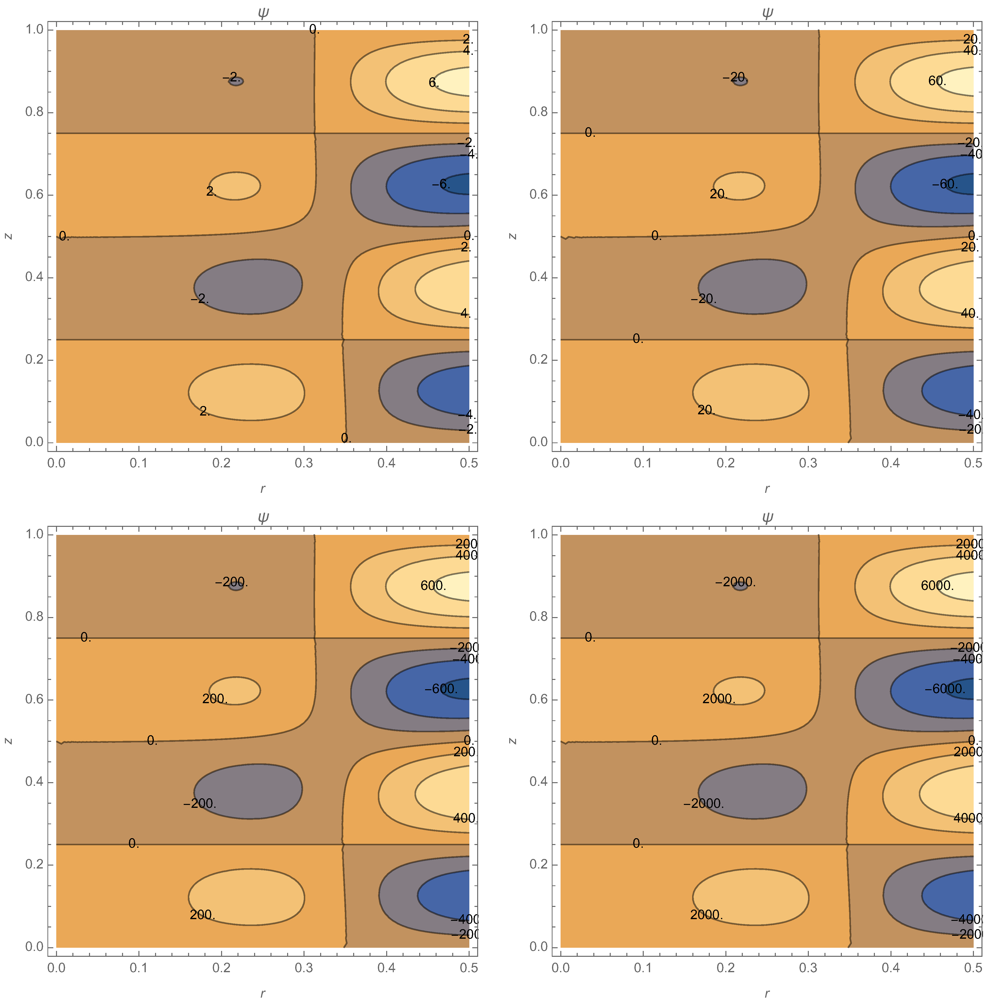
Figure 5.
Study of the perturbation for , i.e., not in the resonance region: (upper left panel); for (upper right panel) and (bottom panel). The contribution of is visible to become larger than the contribution of and, therefore, the linear approximation is not valid above .
Figure 5.
Study of the perturbation for , i.e., not in the resonance region: (upper left panel); for (upper right panel) and (bottom panel). The contribution of is visible to become larger than the contribution of and, therefore, the linear approximation is not valid above .

Figure 6.
Study of the resonance around : 7.3 (upper left panel), 7.35 (upper right panel), 7.36 (bottom left panel), 7.37 (bottom right panel). See text for details.
Figure 6.
Study of the resonance around : 7.3 (upper left panel), 7.35 (upper right panel), 7.36 (bottom left panel), 7.37 (bottom right panel). See text for details.

Figure 7.
Zero-order function for varying in the resonance interval for : (upper left panel), 9.4 (upper right panel), 9.5 (bottom panel). No changes in visible. See text for details.
Figure 7.
Zero-order function for varying in the resonance interval for : (upper left panel), 9.4 (upper right panel), 9.5 (bottom panel). No changes in visible. See text for details.
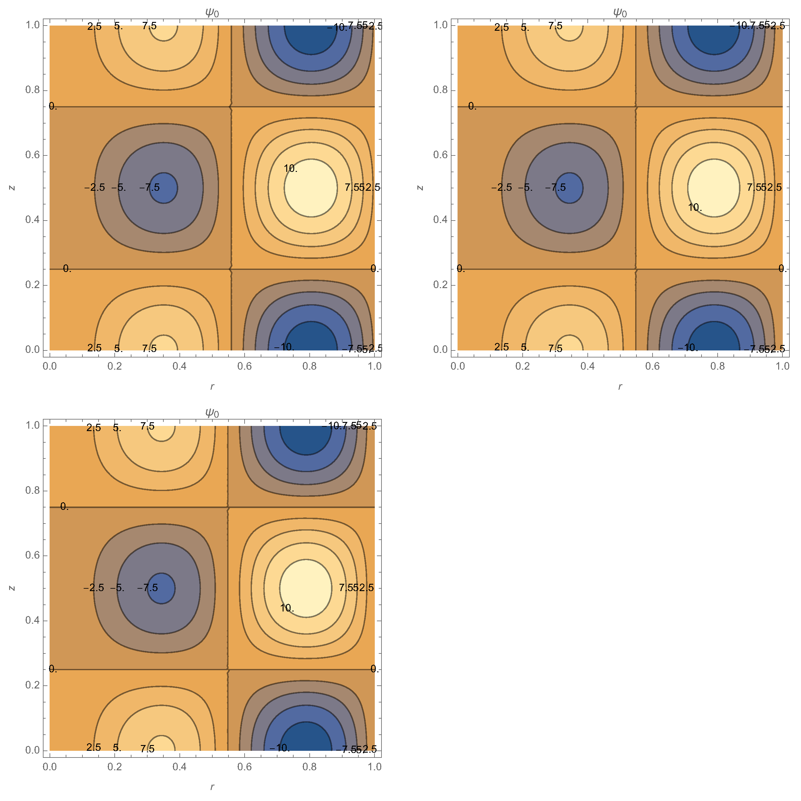
Figure 8.
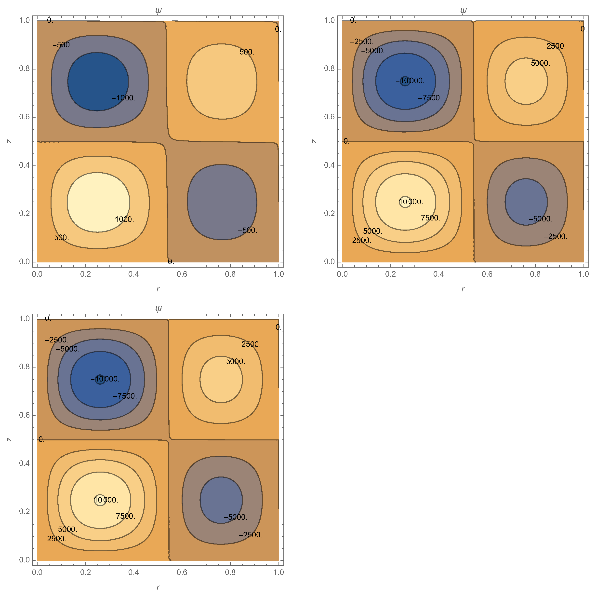
Transition of around the resonance value and : (upper left panel), 9.4 (upper right panel), 9.5 (bottom panel). See text for details.
Figure 8.
Transition of around the resonance value and : (upper left panel), 9.4 (upper right panel), 9.5 (bottom panel). See text for details.

| n | |||
|---|---|---|---|
| 1 | 4,214 | 4.214 | 3.51131 |
| 2 | 4.13661 | 4.13661 | 4.71224 |
| 3 | −3.32075 | 5.66356 | |
| 4 | 7.77266 | −2.9967 | 6.47654 |
Publisher’s Note: MDPI stays neutral with regard to jurisdictional claims in published maps and institutional affiliations. |
© 2022 by the authors. Licensee MDPI, Basel, Switzerland. This article is an open access article distributed under the terms and conditions of the Creative Commons Attribution (CC BY) license (https://creativecommons.org/licenses/by/4.0/).
Share and Cite
MDPI and ACS Style
Tirozzi, B.; Buratti, P. Magnetic Force-Free Theory: Nonlinear Case. Physics 2022, 4, 21-36. https://doi.org/10.3390/physics4010003
AMA Style
Tirozzi B, Buratti P. Magnetic Force-Free Theory: Nonlinear Case. Physics. 2022; 4(1):21-36. https://doi.org/10.3390/physics4010003
Chicago/Turabian StyleTirozzi, Brunello, and Paolo Buratti. 2022. "Magnetic Force-Free Theory: Nonlinear Case" Physics 4, no. 1: 21-36. https://doi.org/10.3390/physics4010003