Enthusiasm and Skepticism: Two Pillars of Science—A Nonextensive Statistics Case

Abstract

Science and its evolution are based on complex epistemological structures. Two of the pillars of such a construction definitively are enthusiasm and skepticism, both being ingredients without which solid knowledge is hardly achieved and certainly not guaranteed. Our friend and colleague Jean Willy André Cleymans (1944–2021), with his open personality, high and longstanding interest for innovation, and recognized leadership in high-energy physics, constitutes a beautiful example of the former. Recently, Joseph I. Kapusta has generously and laboriously offered an interesting illustration of the latter pillar, in the very same field of physics, concerning the very same theoretical frame, namely, nonextensive statistical mechanics and the nonadditive q-entropies on which it is based. I present here a detailed analysis, point by point, of Kapusta’s 19 May 2021 talk and, placing the discussion in a sensibly wider and updated perspective, I refute his bold conclusion that indices q have no physical foundation.

1. Reminiscences Related to Jean Cleymans

I had the privilege of personally meeting Jean Cleymans in two occasions. The first one was at CERN (European Organization for Nuclear Research) for the Heavy Ion Forum held in 2013–2014 to discuss q-statistics in high-energy physics. His experience and scientific weight among his CERN colleagues were noticeable. That was my first visit to CERN, where I stayed a couple of days. The second occasion was during a visit, over several days, to the University of Cape Town, when I also had the opportunity to lecture and discuss, with him and his international research group, on the foundations and applications of nonadditive entropies and nonextensive statistical mechanics.

In the bibliography in [1], over 9000 articles, by nearly 16,000 authors, are registered on this research area, which started in 1988 [2]. Among them, more than one thousand concern high-energy physics (high-energy collisions, possible connections to quantum chromodynamics (QCD), thermofractals, solar physics, astronomy, astrophysics, black holes, cosmology, dark energy; theoretical, observational, experimental). I could find therein fourty two articles by Cleymans and co-authors [3,4,5,6,7,8,9,10,11,12,13,14,15,16,17,18,19,20,21,22,23,24,25,26,27,28,29,30,31,32,33,34,35,36,37,38,39,40,41,42,43,44], spanning over one decade. His longstanding enthusiasm about the subject, at least in what concerns high-energy physics, can be hardly doubted.

2. Analysis of Joseph Kapusta’s Talk “A Primer on Tsallis Statistics for Nuclear and Particle Physics” (19 May 2021)

2.1. Preliminaries

On 19 May 2021, Joseph Kapusta delivered an online talk within the Theoretical Physics Colloquium series that Igor Shovkovy has been hosting at Arizona State University. The talk was entitled “A primer on Tsallis statistics for nuclear and particle physics”, and it is accessible on the Internet [45]. Making it publicly accessible was, in some sense, a fortunate initiative. Indeed, in spite of the fact that my own name appears in the title of the talk, I never received notice of it, rather regretfully. Nevertheless, fortuitously, I could eventually hear, in 27 December 2021, Kapusta’s talk when I became aware of its existence through an anonymous referee report on a project involving q-concepts.

However, why am I giving all these details? Basically, because I agree with the old dictate “silence gives consent” (“qui tacet consentit”), and by no means can I agree with nor remain silent regarding the final conclusions offered by the speaker of that specific talk. Indeed, in what follows, I intend to offer, essentially point by point, an analysis of and a reply to Kapusta’s talk, not only in what concerns the logical implications of his statements and conclusions, but—quite appropriate under the present circumstances—also in what concerns the spirit of the “analyse du discours” [46,47,48]. This is why I focus here on the talk itself and not on the written version, which Kapusta published some months later [49]. Let me add for completeness that, as soon as I became aware of the existence of that talk on YouTube, I proposed an open academic debate between Kapusta and myself, possibly organized within the same or similar frame of the Arizona State University Colloquia series (or any other appropriate forum in fact), but I did not receive back a signal of operational interest. Unfortunately, an opportunity for a free and direct exchange of scientific ideas focusing on a currently active research area was lost.

Before starting, let me by all means make absolutely clear my genuine gratitude to Kapusta for having dedicated a sensible amount of his time and knowledge to analyze and better understand the theory that I proposed over three decades ago (in [2,50] and elsewhere). It is my understanding that, by so proceeding, Kapusta also attempted to serve science along its best lines, in this case through skepticism, as it becomes clear in what follows.

2.2. On the Title of Kapusta’s Talk

The choice of the word “primer” in the title is suggestive. For this word one finds in the Merriam-Webster Dictionary:

-

A small book for teaching children to read;

-

A small introductory book on a subject;

-

A short informative piece of writing.

In the Cambridge Dictionary, one finds:

-

A small book containing basic facts about a subject, used especially when you are beginning to learn about that subject;

-

A basic text for teaching something.

It appears therefore that the word “primer” tends to induce the audience in the sense that basic undeniable facts will be presented, as opposed to opinions or beliefs. In classical philosophical Plato terms, “primer” induces us to think about “episteme” (from the Greek $ϵ\pi \iota \sigma \tau$$\eta \mu \eta$, related to facts) and not about “doxa” (from the Greek $\delta$ó$\xi \alpha$, opinion). But, as the reader can verify, what one hears in various parts of the talk is a blurring between these two concepts, facts and opinion, a blurring between “text” and “context”.

Along a similar vein, the expression “Tsallis and his collaborators” that Kapusta used several times is not exempted from ambiguity. Indeed, there are my collaborators—co-authors, quite frequently—and there are also thousands of scientists (see [1]) who became interested in the subject and have published, along the years, thousands of articles, some of which presenting aspects that I would surely endorse, and others whose statements are certainly not to be confused with my own.

2.3. Nonadditive Entropy $S_q$: Where It Comes from

In his talk, Kapusta declared a couple of times that he did not know where $S_q$ came from. Although spread in the literature for decades, let us summarize in the present occasion where it comes from. Like the Boltzmann–Gibbs entropic functional, it is basically a postulate, as stated in [2]. There is, however, a simple rationale behind it. Let us describe it.

An entropic functional must be invariant under permutation of states; indeed, what matters are the probabilities $\left\{p_i\right\}$ and not the states themselves. The simplest manner which satisfies this property is to involve ${\sum }_{i}f\left(p_i\right)$, and the simplest form for $f\left(p_i\right)$ is just a power-law, i.e., $f\left(p_i\right)\propto p_i^q(q\in \mathbb{R})$. Consistently, the entropic functional being constructed is assumed to be of the form $S_q\left(\left\{p_i\right\}\right)=\Phi \left({\sum }_i{p}_i^q\right)$, with ${\sum }_i{p}_i=1$. The simplest form for $\Phi \left(x\right)$ is to be linear, i.e., $S_q\left(\left\{p_i\right\}\right)=A\left(q\right)+B\left(q\right){\sum }_i{p}_i^q$. Probabilistic certainty should make the entropy to vanish. Therefore, if it is possible for a state j to exist such that $p_j=1$, then ${\sum }_i{p}_i^q=1$, hence $A\left(q\right)+B\left(q\right)=0$. Consequently, $S_q\left(\left\{p_i\right\}\right)=A\left(q\right)(1-{\sum }_i{p}_i^q)$. Now, the whole intuition for the present postulate, inspired in multifractals as declared in [2], is to provide a bias for the state probability. More definitely, to compare $p_i^q$ with $p_i$ for any $p_i\in (0,1)$: $p_i^q>p_i$ if $q<1$, $p_i^q<p_i$ if $q>1$, and finally $p_i^q=p_i$ if $q=1$. As one can see, $q=1$ simply means absence of bias, and this is intuitively assumed to well correspond to the Boltzmann–Gibbs (GB) entropy variable, $S_{\mathrm{BG}}=k{\sum }_i{p}_{i}ln\left(1/p_i\right)$. Therefore, ${lim}_{q\to 1}A\left(q\right)$ must diverge in order to compensate for the fact that ${lim}_{q\to 1}[1-{\sum }_i{p}_i^q]={lim}_{q\to 1}[1-{\sum }_i{p}_i{p}_i^{q-1}]={lim}_{q\to 1}[1-{\sum }_i{p}_i{e}^{(q-1)ln{p}_i}]={lim}_{q\to 1}\{1-{\sum }_i{p}_i[1+(q-1)ln{p}_i]\}={lim}_{q\to 1}(q-1)[-{\sum }_i{p}_{i}ln{p}_i]=0$; moreover, $A\left(q\right)$ must have the dimensions of the constant k, hence be proportional to k. The simplest such possibility satisfying ${lim}_{q\to 1}{S}_q\left\{p_i\right\}=S_{\mathrm{BG}}\left\{p_i\right\}$ is $A\left(q\right)=k/(q-1)$, and we are done. The entropy $S_q$ is therefore defined by

$$\begin{array}{ccc}\hfill S_q\left(\left\{p_i\right\}\right)& \equiv & k\frac{1-{\sum }_{i=1}^W{p}_i^q}{q-1}=k\sum _{i=1}^W{p}_i{ln}_q\frac{1}{p_i}\hfill \\ & =& -k\sum _{i=1}^W{p}_i^q{ln}_q{p}_i=-k\sum _{i=1}^W{p}_i{ln}_{2-q}{p}_i(S_1=S_{\mathrm{BG}}),\hfill \end{array}$$

(1)

where the (monotonically increasing) q-logarithmic function is defined through

$${ln}_{q}z\equiv \frac{z^{1-q}-1}{1-q}({ln}_{1}z=lnz),$$

(2)

with $d{ln}_{q}z/dz=1/z^q$. The quantity $\sigma \left(p\right)\equiv ln(1/p)$ is referred to as “surprise” [51] or “unexpectedness” [52]. It vanishes when the probability p equals unity and diverges when the probability $p\to 0$. One can consistently define q-surprise or q-unexpectedness as ${\sigma }_q\left(p\right)\equiv {ln}_q(1/p)$, hence ${\sigma }_q\left(1\right)=0$ and ${\sigma }_q\left(0\right)$ attains its maximum (infinity if $q\le 1$). With this definition, $S_q$ can be rewritten as follows:

$$S_q=k\sum _{i=1}^W{p}_i{ln}_q(1/p_i)\equiv k\langle {ln}_q(1/p_i)\rangle =k\langle {\sigma }_q\rangle ,$$

(3)

where $\langle \cdots \rangle$ denotes the mean value. Equation (3) satisfies in fact the most general form for a “trace-form” entropic functional, $S_{\Psi }\left(\left\{p_i\right\}\right)=k{\sum }_i{p}_i{ln}_{\Psi }(1/p_i)$, ${ln}_{\Psi }\left(z\right)$ being a generic monotonically increasing function which satisfies ${ln}_{\Psi }\left(1\right)=0$; for details, see [50,53].

In addition, an entropic functional $S(\left\{p_i\right\};\eta )$ is said “composable” if it satisfies, for two probabilistically independent systems A and B, the property $S(A+B)/k=F(S\left(A\right)/k,S\left(B\right)/k;\eta )$, where $\eta$ is a set of fixed indices characterizing the functional (e.g., for $S_q$, it is $\eta \equiv q$); the notation $\left\{0\right\}$ is used here to indicate absence of any such index. $F(x,y;\{\eta \left\}\right)$ is assumed to be a smooth function of $(x,y)$, which depends on a (typically small) set of universal indices $\left\{\eta \right\}$, defined in such a way that $F(x,y;\{0\left\}\right)=x+y$ (additivity), which corresponds to the Boltzmann–Gibbs entropy. Furthermore, $F(x,y;\{\eta \left\}\right)$ is assumed to satisfy $F(x,0;\{\eta \left\}\right)=x$ (null-composability), $F(x,y;\{\eta \left\}\right)=F(y,x;\{\eta \left\}\right)$ (symmetry), $F(x,F(y,z;\left\{\eta \right\});\{\eta \left\}\right)=F\left(F\right(x,y;\left\{\eta \right\}),z;\{\eta \left\}\right)$ (associativity); for details and thermodynamical motivation, see [50,53].

The Enciso–Tempesta theorem [54] proves that $S_q$ is the unique entropic functional which simultaneously is a trace form, composable, and includes the Boltzmann–Gibbs form as a particular instance. These properties play a crucial role in the validity, for all values of q, of the Einstein requirement for likelihood factorization [55]. This important property is consistent with the fact that the Boltzmann–Gibbs statistical mechanics is sufficient but not necessary for the validity of thermodynamics and its Legendre structure.

The word “postulate” used above deserves a comment. For the Boltzmann–Gibbs entropy, it is possible to replace its postulated form by a set of four axioms. That was first shown by Shannon in his celebrated uniqueness theorem [56,57], and later on, in a more elegant form, by Khinchin in his own uniqueness theorem [58,59]. Both theorems have been q-generalized into Santo’s uniqueness theorem [60] and Abe’s uniqueness theorem [61], respectively. Let us finally mention that, in addition to the above uniqueness theorems (Santos in 1997, Abe in 2000, and Enciso and Tempesta in 2017), $S_q$ is unique in other relevant senses as well, namely, the Topsøe factorizability in game theory [62], the Amari–Ohara–Matsuzoe conformally invariant geometry [63] and the Biro–Barnafoldi–Van thermostat universal independence [64].

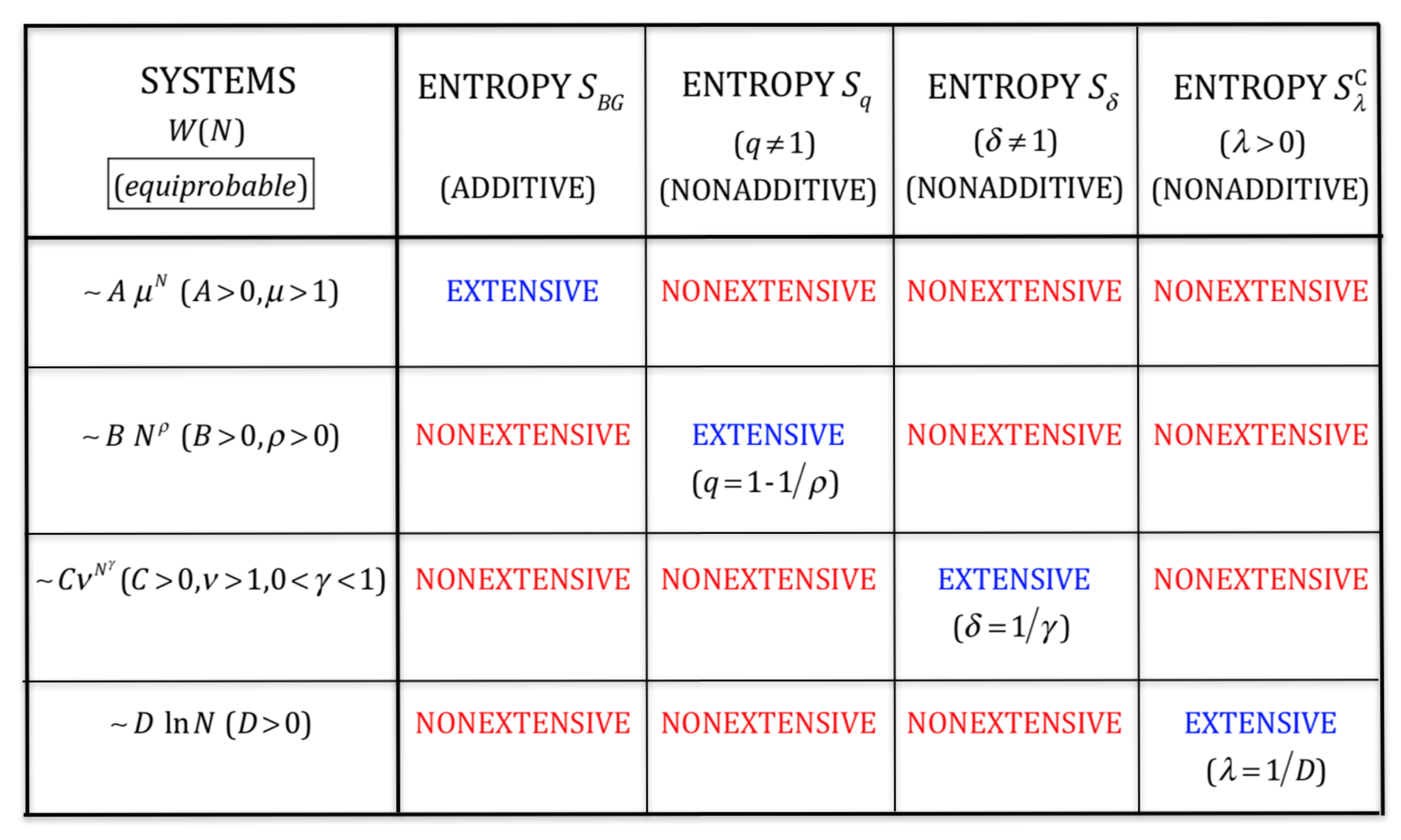
2.4. Additivity versus Extensivity

All the way along his talk, Kapusta did not distinguish—clearly enough, and even at all—the concepts of “extensivity” and “additivity”, applicable to both entropy and energy. This is quite unfortunate since this distinction ought to be made in any introductory talk on the subject. Indeed, it plays a foundational role in nonextensive statistical mechanics. Let us address now these two important notions, focusing specifically on entropic additivity and entropic extensivity.

Following O. Penrose [65], an entropic functional $S\left(\left\{p_i\right\}\right)$ is said “additive” if, for two probabilistically independent systems A and B (i.e., $p_{ij}^{A+B}=p_i^A{p}_j^B)$, one verifies $S(A+B)=S\left(A\right)+S\left(B\right)$, in other words, if

$$S\left(\left\{p_i^A{p}_j^B\right\}\right)=S\left(\left\{p_i^A\right\}\right)+S\left(\left\{p_j^B\right\}\right)$$

(4)

is verified.

Otherwise, $S\left(\left\{p_i\right\}\right)$ is said “nonadditive”. It immediately follows that $S_{\mathrm{BG}}$ is additive. In contrast, $S_q$ satisfies

$$\frac{S_q(A+B)}{k}=\frac{S_q\left(A\right)}{k}+\frac{S_q\left(B\right)}{k}+(1-q)\frac{S_q\left(A\right)}{k}\frac{S_q\left(B\right)}{k},$$

(5)

hence

$$S_q(A+B)=S_q\left(A\right)+S_q\left(B\right)+\frac{1-q}{k}{S}_q\left(A\right)S_q\left(B\right).$$

(6)

Therefore, unless $(1-q)/k\to 0$, $S_q$ is nonadditive.

Let us now address the other important entropic concept, namely, extensivity. An entropy $S\left(N\right)$ is said “extensive” if a specific entropic functional is applied to a specific class of many-body systems with $N=L^d$ particles, where L is its dimensionless linear size and d its spatial dimension, and satisfies the thermodynamical expectation

$$0<\underset{N\to \infty }{lim}\frac{S\left(N\right)}{N}<\infty ,$$

(7)

hence, $S\left(N\right)\propto N$ for $N\gg 1$. Therefore, entropic additivity only depends on the entropic functional, whereas entropic extensivity depends on both the chosen entropic functional and the system itself (i.e., its constituents and the correlations among them).

Let us illustrate this fundamental distinction through four, among infinitely many, equal-probability typical examples of $W\left(N\right)(N\to \infty )$, where W is the total number of possibilities whose probability does not vanish.

• Exponential class $W\left(N\right)\sim A{\mu }^N(A>0;\mu >1)$:
  This is the typical case within the Boltzmann–Gibbs theory. One gets: $S_{\mathrm{BG}}\left(N\right)=klnW\left(N\right)\sim Nln\mu +lnA\propto N$, therefore, $S_{\mathrm{BG}}$ is extensive, as thermodynamically required.
• Power-law class $W\left(N\right)\sim B{N}^{\rho }(B>0;\rho >0)$:
  One should not use $S_{\mathrm{BG}}$ since it implies $S_{\mathrm{BG}}\left(N\right)=klnW\left(N\right)\sim \rho lnN+lnB\propto lnN$, thus violating thermodynamics. One verifies instead that $S_{q=1-1/\rho }\left(N\right)=k{ln}_{q=1-1/\rho }W\left(N\right)$$\propto N$, as thermodynamically required.
• Stretched exponential class $W\left(N\right)\sim C{\nu }^{N^{\gamma }}(C>0;\nu >1;0<\gamma <1)$:
  In this case, no value of q exists which would yield an extensive entropy $S_q$. One can instead use $S_{\delta }\equiv k{\sum }_{i=1}^W{p}_i{[ln1/p_i]}^{\delta }$ [50] with $\delta =1/\gamma$. Indeed, $S_{\delta =1/\gamma }\left(N\right)=k{[lnW\left(N\right)]}^{1/\gamma }\propto N$, as thermodynamically required.
• Logarithmic class $W\left(N\right)\sim DlnN(D>0)$:
  In this case, no values of $(q,\delta )$ exist which are able to yield an extensive entropy $S_{q,\delta }\equiv k{\sum }_i{p}_i[{ln}_q{(1/p_i]}^{\delta }$ [66]. Instead, one can use the Curado entropy [53], $S_{\lambda }^C\left(N\right)=k\left[e^{\lambda W\left(N\right)}-e^{\lambda }\right]$ with $\lambda =1/D$. Indeed, one can verify that $S_{\lambda =1/D}^C\left(N\right)\propto N$, as thermodynamically required.

These four paradigmatic classes are described in Figure 1.

At this point, it is pertinent to remind Einstein’s 1949 comment [67]: “A theory is the more impressive the greater the simplicity of its premises is, the more different kinds of things it relates, and the more extended is its area of applicability. Therefore, the deep impression that classical thermodynamics made upon me. It is the only physical theory of universal content concerning which I am convinced that, within the framework of applicability of its basic concepts, it will never be overthrown”.

To better understand the strength of these words, a metaphor can be used. Within Newtonian mechanics, there is the known Galilean composition of velocities, $v_{13}=v_{12}+v_{23}$. In special relativity, this law is generalized into $v_{13}=[v_{12}+v_{23}]/[1+v_{12}{v}_{23}/c^2]$, where c is the speed of light, thus violating additivity. Why did Einstein abandon the simple linear composition of Galileo? Because he had a higher goal, namely, to unify mechanics and Maxwell’s electromagnetism, and, for this, he had to impose the invariance with regard to the Lorentz transformation. One can, thus, see the violation of the linear Galilean composition as a small price to pay for a major endeavor. Similarly, what is expressed in Figure 1, is that q-generalizing the linear composition law of $S_{\mathrm{BG}}$, with regard to independent systems, into the nonlinear composition (5) may be seen as a small price to pay for a major endeavor, namely, to always satisfy the Legendre structure of thermodynamics. However, it is mandatory to register here that such viewpoint is nevertheless not free from controversy, in spite of its simplicity. For example, the known expression of Bekenstein and Hawking for the entropy for a black hole is proportional to its surface instead of to its volume, therefore violating the above requirement if the black-hole is assumed to be a three-dimensional object; see [66].

Before leaving this point, it is fair to mention that Kapusta’s lack of distinction between entropic extensivity and entropic additivity would not be particularly surprising, were it not for his own perception of his talk as a “primer“. In any case, such confusion constitutes, still today, no exception in the literature even if my co-author Murray Gell-Mann and myself started around 2003 to emphasize the distinction in my book [50] and in our paper [68].

2.5. On the Nature of the Constraints Used for Entropic Optimization

The relevance of the invariance, under a zero-energy shift at fixed inverse effective temperature ${\beta }_q$, of the distribution of probabilities extremizing $S_q$ took, from [2] through [69] to [70], close to ten years to become clarified. As pedagogically explained by Kapusta, this process led, through types I and II, to the type III or third path, which was specially focused in his talk. The equivalence, under appropriate transformations of q and, consistently, of the Lagrange parameters $(\alpha ,\beta )$, associated with these three paths was later on established in [71,72]. Indeed, the possibility of linking $S_{2-q}$ (instead of $S_q$) with the extremizing q-exponential distribution and linear constraints such as ${\sum }_i{p}_i{E}_i=\langle E\rangle$ (instead of the nonlinear constraint ${\sum }_i{p}_i^q{E}_i/{\sum }_i{p}_i^q={\langle E\rangle }_q$) was later on used in [73,74,75,76,77,78,79,80,81,82] on the basis of identities (1), and has nowadays become quite popular due to its operational simplicity. This link is based on a nonlinear Fokker–Planck Equation (with nonlinear exponent $(2-q)$) in the presence of a confining potential [83,84]. This equation has, as its basic stationary state, a q-Gaussian and not a $(2-q)$-Gaussian. Further examples exhibiting the same type of duality are available at [85,86].

Let us mention at this stage that several central related issues were regretfully ignored in Kapusta’s talk, namely:

• The peculiar way the nonlinear constraint of type III was phrased by the speaker left floating in the audience (which even repeated this later on, with the tacit agreement of the speaker) that this assumption was violating the theory of probabilities. There is no such thing.
  Indeed, the above nonlinear constraint in $p_i$ is completely equivalent to a linear constraint expressed in terms of ${\sum }_i{P}_i^{\left(q\right)}{E}_i$ where $P_i^{\left(q\right)}\equiv p_i^q/{\sum }_j{p}_j^q$ (hence $p_i={\left(P_i^{\left(q\right)}\right)}^{1/q}/{\sum }_j{\left(P_j^{\left(q\right)}\right)}^{1/q}$, with ${\sum }_i{p}_i={\sum }_i{P}_i^{\left(q\right)}=1$) is the so-called “escort distribution,” defined in the theory of probabilities; see [87] and references therein.
• The requirement for system-independence for the adopted extremization procedure consists of having for both the norm constraint, expressed in terms of ${\sum }_i{p}_i$, and the energy constraint, expressed in terms of ${\sum }_i{P}_i^{\left(q\right)}{E}_i$, one and the same upper admissible value for q. Let us illustrate this through an example. If the set of eigenvalues $\left\{E_i\right\}$ are nondegenerate, the extremizing q-exponential distribution with $q>1$ asymptotically behaves as $1/E_i^{1/(q-1)}$. Therefore, its norm is well defined up to $q=2$. The same happens with the constraint ${\sum }_i{P}_i^{\left(q\right)}{E}_i$. Indeed, it asymptotically behaves as $E_i/E_i^{q/(q-1)}=1/E_i^{1/(q-1)}$, hence it has the same upper bound admissibility, i.e., once again $q=2$. In strong variance, if one were to use here the usual ${\sum }_i{p}_i{E}_i$ constraint, the asymptotic behavior would be given by $E_i/E_i^{1/(q-1)}$, hence its upper admissible value would be $q=3/2$, which differs from the norm admissibility value, $q=2$. The general importance of this point is lengthily discussed in [88].
• In the q-generalized central limit theorem and Lévy–Gnedenko’s limit theorem [89,90], the escort mean values emerge naturally from the mathematical operations themselves.
• All mean values must be mathematically defined for the fat-tailed $q>1$ distributions. This does happen with the appropriate escort averages but fails with the normal linear averages. A simple numerical example with q-Gaussians and its astonishing practical consequences are illustrated in [91].

2.6. On Ad Hoc Constraints for Optimizing the Entropy

Kapusta referred, in a kind of appreciative style, to a 2004 argument by Zanette and Montemurro [92], which would “disqualify” $S_q$ as a “physical” entropy. It refers to the trivial mathematical fact that by adjusting in an ad hoc manner the constraints under which the entropy optimization is to be done, one can obtain virtually any desired distribution. This mathematical feature applies to all admissible entropic functionals (including $S_{\mathrm{BG}}$) and has been an overcome issue for a long time. Indeed, already in 1983, Montroll and Shlesinger [93] exhibited how the nontrivial constraint can be adapted in order to obtain Lévy distributions from the classical Boltzmann–Gibbs entropy. The author’s epistemological dissatisfaction is evident in the paper. Indeed, one is forced to first know the distribution that is aimed, and then, through a sort of reverse engineering, write down the nontrivial constraint in order to get it. This is actually possible for any entropic functional, as mentioned above, but provides no useful information at all. Constraints within information theory are not to be freely manipulated: they must reflect constants of motion and similar quantities. For a simple real random variable x, they must restrict to robust constraints such as the values of $\langle x\rangle$ and/or of $\langle x^2\rangle$. It is up to the entropic functional, and not to the ad hoc constraints, to do the most meaningful and nontrivial job.

We argue here that, since it is known to be so for any entropic form and, in particular, for the (additive) Boltzmann–Gibbs entropy, $S_{\mathrm{BG}}$ (see [94]), the critique brings absolutely no novelty to the area. In other words, it has nothing special to do with the entropy $S_q$. In favor of the constraints based on the usual simple variables (typically, the averaging of the random variable $x_i$ or of $x_i^2$, where $x_i$ is to be identified according to the nature of the system), we argue, and this for all entropic forms, that they can hardly be considered as arbitrary, as the authors of [92] seemingly consider. Indeed, once the natural variables of the system have been identified (e.g., constants of motion of the system, such as the energy for Hamiltonian systems), the variable itself and, in some occasions, its square are the most basic quantities to be constrained. Such constraints are used in hundreds (perhaps thousands) of useful applications outside (and also inside) thermodynamical systems, along the information theory lines of Jaynes and Shannon, and more recently of A. Plastino and others. Furthermore, this is so for $S_{\mathrm{BG}}$, $S_q$, and any other entropic form. Rebuttals of the Zanette and Montemurro outdated criticism can be found in [50,95,96].

As a final comment, let us mention that statistical mechanics is much more that just a stationary-state (e.g., thermal equilibrium) distribution. Indeed, under exactly the same constraints, the optimization of $S_{\mathrm{BG}}$ and ${\left(S_{\mathrm{BG}}\right)}^3$ yields the same distribution. This is not a sufficient reason for using ${\left(S_{\mathrm{BG}}\right)}^3$ instead of $S_{\mathrm{BG}}$ in a thermostatistical theory which must also satisfy various thermodynamical requirements, including its Legendre-transformation structure.

2.7. Thermodynamics and Legendre Transformations

Before focusing on the Legendre structure itself, let us review some long-known facts concerning long-range interactions. Let us consider a d-dimensional classical many-body system with, e.g., attractive two-body isotropic interactions decaying with a dimensionless distance $r\ge 1$ as $-A/r^{\alpha }$ ($A>0$, $\alpha \ge 0$), and with an infinitely repulsive potential for $0\le r\le 1$. At zero temperature T, the total kinetic energy vanishes, and the potential energy per particle is proportional to ${\int }_1^{\infty }dr{r}^d{r}^{-\alpha }$. This quantity converges if $\alpha /d>1$ and diverges otherwise. These two regimes are from now on referred to as “short-range” and “long-range” interactions, respectively; see Figure 2.

Furthermore, they can be shown to, respectively, correspond, within the Boltzmann–Gibbs theory, to finite and divergent partition functions. This is indeed the point that was addressed by Gibbs himself [97]: “In treating of the canonical distribution, we shall always suppose the multiple integral in Equation (92) [the partition function, as it is called nowadays] to have a finite value, as otherwise the coefficient of probability vanishes, and the law of distribution becomes illusory. This will exclude certain cases, but not such apparently, as will affect the value of our results with respect to their bearing on thermodynamics. It will exclude, for instance, cases in which the system or parts of it can be distributed in unlimited space [...]. It also excludes many cases in which the energy can decrease without limit, as when the system contains material points which attract one another inversely as the squares of their distances. [...]. For the purposes of a general discussion, it is sufficient to call attention to the assumption implicitly involved in the Formula (92)”.

In a vein slightly differing from the standard Boltzmann–Gibbs recipe, which would demand integration up to infinity in ${\int }_1^{\infty }dr{r}^d{r}^{-\alpha }$, let us assume that the N-particle system is roughly homogeneously distributed within a limited sphere. Then, the potential energy per particle scales as follows:

$$\frac{U_{\mathrm{pot}}\left(N\right)}{N}\propto -A{\int }_1^{N^{1/d}}dr{r}^{d-1}{r}^{-\alpha }=-\frac{A}{d}{N}^{*},$$

(8)

with

$$N^{☆}\equiv \frac{N^{1-\alpha /d}-1}{1-\alpha /d}={ln}_{\alpha /d}N\sim \left\{\begin{array}{ccc}{\displaystyle \frac{1}{\alpha /d-1}}\hfill & \hfill & \mathrm{if}\alpha /d>1;\hfill \\ \\ lnN\hfill & \hfill & \mathrm{if}\alpha /d=1;\hfill \\ \\ {\displaystyle \frac{N^{1-\alpha /d}}{1-\alpha /d}}\hfill & \hfill & \mathrm{if}0\le \alpha /d<1.\hfill \end{array}\right.$$

(9)

Therefore, in the $N\to \infty$ limit, $U_{pot}\left(N\right)/N$ approaches a constant ($\propto -A/(\alpha -d)$) if $\alpha /d>1$, and diverges like $N^{1-\alpha /d}/(1-\alpha /d)$ if $0\le \alpha /d<1$ (it diverges logarithmically if $\alpha /d=1$). In other words, the total potential energy is extensive for short-range interactions ($\alpha /d>1$), and nonextensive for long-range interactions ($0\le \alpha /d\le 1$). Satisfactorily enough, Equation (9) recovers the characterization with ${\int }_1^{\infty }dr{r}^d{r}^{-\alpha }$ in the limit $N\to \infty$, but it has the great advantage of providing, for finite N, a finite value. This fact is now shown to enable us to properly scale the macroscopic quantities in the thermodynamic limit ($N\to \infty$), for all values of $\alpha /d\ge 0$ and not only for $\alpha /d>1$ (as in textbooks of thermodynamics, even if the point is too frequently not made explicitly).

The mathematical structure of classical thermodynamics is based on the Legendre transforms. It is not sufficiently realized that thermodynamics does not depend on microscopic details only for short-range interactions. As is illustrated here below, it does depend on quantities such as $(\alpha ,d)$ for long-range interactions. Quoting Landsberg [98]: “The presence of long-range forces causes important amendments to thermodynamics, some of which are not fully investigated as yet”.

Let us consider a d-dimensional homogeneous and isotropic classical fluid constituted by magnetic particles in thermodynamical equilibrium. Its Gibbs free energy is then:

$$\begin{array}{ccc}\hfill G(N,T,p,\mu ,H)& =& U(N,T,p,\mu ,H)-TS(N,T,p,\mu ,H)\hfill \\ & +& pV(N,T,p,\mu ,H)-\mu N-HM(N,T,p,\mu ,H),\hfill \end{array}$$

(10)

where $(T,p,\mu ,H)$ correspond, respectively, to the temperature, pressure, chemical potential and external magnetic field, U is the internal energy, S is the entropy, V is the volume, N is the number of particles, and M the magnetization.

If the interactions are short-ranged, i.e., if $\alpha /d>1$, one can divide this equation by N and then take the $N\to \infty$ limit. One straightforwardly obtains:

$$g(T,p,\mu ,H)=u(T,p,\mu ,H)-Ts(T,p,\mu ,H)+pv(T,p,\mu ,H)-\mu -Hm(T,p,H),$$

(11)

where $g(T,p,\mu ,H)\equiv {lim}_{N\to \infty }G(N,T,p,\mu ,H)/N$, and analogously for the other variables of the equation.

If the interactions are long-ranged instead, i.e., if $0\le \alpha /d\le 1$, all the terms of expression (11) diverge, hence, thermodynamically speaking, they are nonsense. Consequently, the generically correct procedure for all values of $\alpha /d\ge 0$, must conform to the following lines:

$$\begin{array}{ccc}\hfill \underset{N\to \infty }{lim}\frac{G(N,T,p,\mu ,H)}{N{N}^{☆}}=\underset{N\to \infty }{lim}\frac{U(N,T,p,\mu ,H)}{N{N}^{☆}}-\underset{N\to \infty }{lim}\left[\frac{T}{N^{☆}}\frac{S(N,T,p,\mu ,H)}{N}\right]& & \hfill \\ \hfill +\underset{N\to \infty }{lim}\left[\frac{p}{N^{☆}}\frac{V(N,T,p,\mu ,H)}{N}\right]-\underset{N\to \infty }{lim}\frac{\mu }{N^{☆}}-\underset{N\to \infty }{lim}\left[\frac{H}{N^{☆}}\frac{M(N,T,p,\mu ,H)}{N}\right],& \end{array}$$

(12)

hence,

$$\begin{array}{ccc}\hfill g(T^{☆},p^{☆},{\mu }^{☆},H^{☆})& =& u(T^{☆},p^{☆},{\mu }^{☆},H^{☆})-T^{☆}s(T^{☆},p^{☆},{\mu }^{☆},H^{☆})\hfill \\ & & +p^{☆}v(T^{☆},p^{☆},{\mu }^{☆},H^{☆})-{\mu }^{☆}-H^{☆}m(T^{☆},p^{☆},{\mu }^{☆},H^{☆}),\hfill \end{array}$$

(13)

where the definitions of $T^{☆}$ and of all the other variables are self-explanatory (e.g., $T^{☆}\equiv {lim}_{N\to \infty }[T/N^{☆}]$ and $s(T^{☆},p^{☆},{\mu }^{☆},H^{☆})\equiv {lim}_{N\to \infty }[S(N,T,p,\mu ,H)/N]$). In other words, in order to have finite thermodynamic equations of states, one must, in general, express them in the $(T^{☆},p^{☆},{\mu }^{☆},H^{☆})$ variables. If $\alpha /d>1$, this procedure recovers the usual equations of states, and the usual extensive ($G,U,S,V,N,M$) and intensive ($T,p,\mu ,H$) thermodynamic variables. However, if $0\le \alpha /d\le 1$, the situation is more complex, and three instead of the traditional two classes of thermodynamic variables emerge. One may call them extensive ($S,V,N,M$), pseudoextensive ($G,U$) (superextensive in the present case) and pseudointensive ($T,p,\mu ,H$) (superintensive in the present case) variables. All the energy-type thermodynamical variables ($G,F,U$), F being the Helmholtz free energy, give rise to pseudoextensive ones, whereas those which appear in the usual Legendre thermodynamical pairs give rise to pseudointensive ones ($T,p,\mu ,H$) and extensive ones ($S,V,N,M$). Let us emphasize that $(S,V,N,M)$ are extensive in all cases; see Figure 3. The exactness of all these scalings has been repeatedly verified in the literature for diverse concrete physical systems, such as fluids, magnets, polymers and percolation; see [50] and references therein.

Let us also emphasize that, consistently:

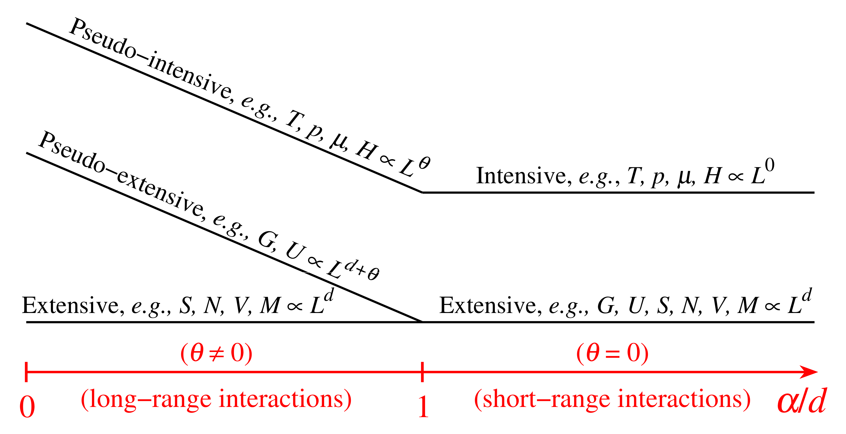
• The ratio of any two pseudointensive variables ($T,p,\mu ,H,\cdots$), e.g., $p/T$, is intensive in all cases;
• The ratio of any pseudoextensive variable $(G,F,U)$ with any pseudointensive variable, e.g., $U/T$, is extensive in all cases;
• A most important implication is that, in expressions such as $e_q^{-{\beta }_q{\mathcal{H}}_N}$ where ${\mathcal{H}}_N$ is an N-body Hamiltonian, the argument ${\beta }_q{\mathcal{H}}_N$ is extensive in all cases. This plays a crucial role in the possible q-generalization of what is currently referred to as the large deviation theory. Indeed, the extensivity of ${\beta }_q{\mathcal{H}}_N$ appears to mirror, in all cases, the extensivity of the total entropy involved in $r_{q}N$, $r_q$ being the ratio function (defined within the Large Deviation probability $P\left(N\right)=P\left(0\right)e_q^{-r_{q}N}$), seemingly always related to some relative nonadditive entropy per particle [102,103,104,105,106].

2.8. Boltzmann Equation

Kapusta also focused on the current Boltzmann equation associated with the $a+b\leftrightarrow c+d$ reaction. He specifically presented and discussed

$$\begin{array}{ccc}\hfill \frac{d{f}_a}{dt}& =& \int \frac{d^3{p}_b}{{\left(2\pi \right)}^3}\frac{d^3{p}_c}{{\left(2\pi \right)}^3}\frac{d^3{p}_d}{{\left(2\pi \right)}^3}\{\frac{1}{1+{\delta }_{cd}}W(c+d\to a+b)f_c{f}_d\times [1+{(-1)}^{2s_a}{f}_a][1+{(-1)}^{2s_b}{f}_b]\hfill \\ & & -\frac{1}{1+{\delta }_{ab}}W(a+b\to c+d)f_a{f}_b\times [1+{(-1)}^{2s_c}{f}_c][1+{(-1)}^{2s_d}{f}_d]\},\hfill \end{array}$$

(14)

where $s_i$ and $p_i$ are the spin and 3-momentum of the ith particle, t is the time, and ${\delta }_{ij}$ is the Kronecker delta, where $i=a,b,c,$ and d. In thermal equilibrium, $d{f}_a/dt=0$, $f_a$ has the usual Boltzmann–Gibbs expression, and the energy conservation, ${\omega }_a+{\omega }_b={\omega }_c+{\omega }_d$ is guaranteed, both in the quantum and the classical cases. In the classical limit, one finds the usual expression, $f=e^{-\beta \omega }$.

Kapusta conveniently pointed out that replacing, in the Boltzmann equation, the traditional molecular chaos hypothesis (stosszahlansatz) factorization, $f_c{f}_d$ by ${[f_c^{1-q}+f_d^{1-q}-1]}^{1/(1-q)}$ (and analogously for $f_a{f}_b$) [107,108], leads to the q-exponential distribution as the stationary state, also satisfying simultaneously the energy conservation, ${\omega }_a+{\omega }_b={\omega }_c+{\omega }_d$. However, he shared that, essentially, he did not know where that specific replacement came from.

Ulrich Heinz, in the audience, shared with friendly complicity that “After so many papers that I have rejected on Tsallis statistics, I am really happy to hear your talk”. About that, not having been communicated in any way that this talk was going to happen online so that I could participate myself, I have no other comment than to say that it is allowed to think that, maybe, not all those rejections were justified. On the other hand, interestingly enough, Heinz also shared that he could, however, “live” with a properly generalized Boltzmann equation.

Let us clarify, at this point, that ${[f_c^{1-q}+f_d^{1-q}-1]}^{1/(1-q)}$ is known to correspond, for $q\ne 1$, to a specific (and apparently not rare at all in nature) class of strong correlations between the relevant random variables.

The product $xy$ of two real numbers has been conveniently generalized as the following q-product [109,110]:

$$x{\otimes }_{q}y\equiv e_q^{{ln}_{q}x+{ln}_{q}y}={\left[x^{1-q}+y^{1-q}-1\right]}_{+}^{\frac{1}{1-q}}(x\ge 0,y\ge 0),$$

(15)

where ${[\cdots ]}_{+}=[\cdots ]$ if $[\cdots ]>0$ and vanishes otherwise. Let us list some of its main properties:

• It recovers the standard product as the $q=1$ particular instance, i.e.,

  $$x{\otimes }_{1}y=xy;$$

  (16)
• It is commutative for all values of q, i.e.,

  $$x{\otimes }_{q}y=y{\otimes }_{q}x;$$

  (17)
• It is additive under q-logarithm for all values of q, i.e.,

  $${ln}_q\left(x{\otimes }_{q}y\right)={ln}_{q}x+{ln}_{q}y,$$

  (18)
  (referred to as “extensivity”), whereas let us remind that

  $${ln}_q\left(xy\right)={ln}_{q}x+{ln}_{q}y+(1-q)\left({ln}_{q}x\right)\left({ln}_{q}y\right)$$

  (19)
  (referred to as “nonadditivity”).
  Consistently,

  $$e_q^x{\otimes }_q{e}_q^y=e_q^{x+y},$$

  (20)

  whereas

  $$e_q^x{e}_q^y=e_q^{x+y+(1-q)xy};$$

  (21)
• It is associative for all values of q, i.e.,

  $$x{\otimes }_q\left(y{\otimes }_{q}z\right)=\left(x{\otimes }_{q}y\right){\otimes }_{q}z=x{\otimes }_{q}y{\otimes }_{q}z={(x^{1-q}+y^{1-q}+z^{1-q}-2)}^{1/(1-q)};$$

  (22)
• It admits unity for all values of q, i.e.,

  $$x{\otimes }_{q}1=x;$$

  (23)
• It admits zero under certain conditions, namely

  $$\begin{array}{c}\hfill x{\otimes }_{q}0=\left\{\begin{array}{c}0\mathrm{if}\left(q\ge 1\mathrm{and}x\ge 0\right)\mathrm{or}\mathrm{if}\left(q<1\mathrm{and}0\le x\le 1\right),\\ \\ {\left(x^{1-q}-1\right)}^{\frac{1}{1-q}}\mathrm{if}q<1\mathrm{and}x>1;\end{array}\right.\end{array}$$

  (24)
• It is distributive with regard to the generalized associative sum analyzed in [111], namely,

  $$x{\oplus }^{\left(q\right)}y\equiv e_q^{ln[e^{{ln}_{q}x}+e^{{ln}_{q}y}]}={\left\{1+(1-q)ln\left[e^{\frac{x^{1-q}-1}{1-q}}+e^{\frac{y^{1-q}-1}{1-q}}\right]\right\}}^{1/(1-q)}.$$

  (25)

In other words, the q-product (15) satisfies all the standard requirements of a full algebraic structure.

Consistently, on the basis of this product, it is possible to generalize, for $q\ge 1$, the Fourier transform of a non-negative function $f\left(x\right)$ as follows [89,90]:

$$F_q\left[f\right]\left(\xi \right)\equiv \int dx{e}_q^{i\xi x}{\otimes }_{q}f\left(x\right)F_q\left[f\right]\left(\xi \right)={\int }_{-\infty }^{\infty }dx{e}_q^{i\xi x{\left[f\left(x\right)\right]}^{q-1}}f\left(x\right).$$

(26)

It is transparent that this transformation is, for $q\ne 1$, nonlinear. Indeed, if $f\left(x\right)\to \lambda f\left(x\right)$, $\lambda$ being any constant, one verifies that $F_q\left[\lambda f\right]\left(\xi \right)\ne \lambda F_q\left[f\right]\left(\xi \right)$. This generalization of the standard Fourier transform $F_1\left[f\right]\left(\xi \right)$ was introduced in order to have a remarkable property: it transforms q-Gaussians into q-Gaussians. Indeed, one verifies:

$$F_q\left[B_q\sqrt{\beta }{e}_q^{-\beta x^2}\right]\left(\xi \right)=e_{q_1}^{-{\beta }_1{\xi }^2},$$

(27)

where

$$(q_1,{\beta }_1)=\left(\frac{1+q}{3-q},\frac{3-q}{8{\beta }^{2-q}{B}_q^{2(q-1)}}\right)(1\le q<2),$$

(28)

$B_q$ being an appropriate normalizing quantity. Within this frame, and others as well, the central limit theorem has been generalized [89,90], showing that, while averaging a large number of random variables within a wide class of nonlocal correlations (yet only partially explored), q-Gaussians emerge as attractors in the space of distributions. This provides an epistemological basis for understanding why there are so many q-Gaussians (and, consistently, so many q-exponentials) in nature; for more details and proofs, see [112]. Moreover, in what concerns the physical significance of the q-product (15) in relation with the Boltzmann transport equation, detailed arguments along a different line are presented as well in [113].

Another relevant line of mathematical research concerns the relations within various sets of q-indices (e.g., q-triplets) that very frequently emerge in complex systems [68,114].

Let us also mention that, in the context of relaxation times related to the Boltzmann equation, Heinz inquired about an interesting question, namely, whether there is any argument yielding q-statistics as an outcome of corresponding dynamics. On general grounds, this not an easy question. However, it is surely useful to have in mind that, in the same way the solution of $dx/dt=-x/\tau$ (with $x\left(0\right)=1$) is $x=e^{-t/\tau }$, the solution of $dx/dt=-x^q/{\tau }_q$ (with $x\left(0\right)=1$) is $x=e_q^{-t/{\tau }_q}$ [115].

At this point, it might be useful to mention that possible q-generalizations of the connections with the Kadanoff–Baym approach have been advanced in [116,117]. Finally, a first step focusing on the Bogoliubov–Born–Green–Kirkwood–Yvon (BBGKY) hierarchy has been introduced in [118].

2.9. On the Second Principle of Thermodynamics

Masoud Shokri, in the audience, inquired about the validity of the second principle for $q\ne 1$. By all means, it appears to be valid in the same way as for the Boltzmann–Gibbs case ($q=1$). The following (nonexhaustive) list of arguments that are available in the literature can be mentioned:

• It has been proved that a detailed balance implies the time irreversibility of $S_q$ [119].
• The celebrated Clausius inequality, $\delta Q/T\le dS$, is consistent with the second principle. It has been shown [120] that it remains valid as it stands for $q>1$ as well.
• The validity of the H-theorem has been proved for a wide class of classical d-dimensional many-body overdamped systems including repulsive short-range two-body interactions [73,74,75,76,77,78,79,80,81,82].
• The H-theorem has been proved for $S_q$ by imposing Galilean-invariance on a Boltzmann lattice model which discretizes the Navier–Stokes equation. The unique value of q is determined by the structure of the Bravais lattice that is being focused on; for more details, see [121,122].
• The time evolution of the entropy for low-dimensional maps, or, actually, the Pesin identities, do certainly not prove the validity of the second principle. However, the fact that the behavior is quite similar (see [123,124,125] and references therein) for, e.g., the logistic map at the most chaotic value of its external parameter (with $q=1$) and at the Feigenbaum point (with $q=0.2445\cdots$) does provide a suggestive indication.

2.10. On the Zeroth Principle of Thermodynamics

Boris Tomasik, in the audience, inquired about the concept of thermal contact among systems in equilibrium, thus tacitly about its transitivity. This highly interesting issue points essentially towards the content of the zeroth principle.

In various overdamped classical d-dimensional many-body systems including short-range repulsive interactions, it has been possible to analytically calculate and numerically verify the validity of q-statistics, focusing on space and velocity distributions, equations of states, Carnot cycle, H-theorem, effective temperature, and the zeroth principle of thermodynamics [73,74,75,76,77,78,79,80,81,82]. For example, for repulsive interactions proportional to $1/r^{\alpha }$, it can be proved [82] that the distribution of positions is a q-Gaussian with $q=1-\alpha /d<1$, which, in the limit $\alpha /d\to 1$, recovers the type-II superconductor result $q=0$ [73,74,75]. This class of systems constitute a rare case where nearly all q-thermostatistical quantities can be analytically calculated.

However, this may be considered as the infancy of a general proof of the validity of the zeroth principle. Its general discussion remains to be done, and it is related, within q-statistics, to the concept of “effective temperature” itself. Indeed, in the above overdamped systems, two different temperatures coexist, namely, the kinetic and effective temperatures. The former is based on the distributions of velocities, whereas the latter is based on the spatial distribution. This is in fact quite analogous to what happens in granular packing, sandpiles and the like, where one is forced to distinguish the kinetic temperature from the structural one [126]. This is in variance with Kapusta’s repeated expression referring to “the true temperature”, without really explaining in physically neat and indisputable terms what “temperature” (or “inverse $\beta$”) he is referring to. It is allowed to think that he only has in his mind the usual kinetic concept of temperature, thus ignoring that, in many complex systems, more than one temperature typically emerges; see, e.g., [73,74,75,76,77,78,79,80,81,82].

2.11. Indices q: First-Principle Characterization of Universality Classes, or Merely Efficient Fitting Parameters?

Kapusta’s ultimate question consists of establishing whether or not the indices q have a first-principle physical basis. He eventually answers by the negative. Let us point out here that a definitively opposite perspective emerges through the (nonexhaustive) list of counter-examples, either from first principles or at a clear-cut mesoscopic level, in diverse complex systems, including high-energy collisions. Let us emphasize that it is well understood that the analytical determination of the q values is, in most of the cases—but fortunately not all!—mathematically intractable.

• First-principle quantum field theory calculation of q for a one-dimensional quantum many-body Hamiltonian system: One such example is the quantum phase transition at $T=0$ criticality for the $d=1$ first-neighbor Ising ferromagnet in the presence of a transverse magnetic field, and similar quantum systems characterized by a central charge, $c\ge 0$. A subsystem of large linear size L of an infinitely long such chain satisfies $S_{\mathrm{BG}}\left(L\right)\propto lnL$, which is nonextensive and therefore violates the Legendre structure of thermodynamics. It turns out, however, that a unique value of q exists such that $S_q\left(L\right)\propto L$, thus satisfying thermodynamics. Its value is given by [127]

  $$q=\frac{\sqrt{9+c^2}-3}{c},$$

  (29)

  which is depicted in Figure 4. As one can see, q characterizes here the thermodynamically admissible entropies associated with the criticality universality classes of many-body systems, defined by the central charge c.
• Zero-Lebesgue occupancy of the probability space in the $N\to \infty$ limit of a system with strongly correlated random binary variables [68]: it is verified that $S_q$ is extensive for a unique value of q, namely,

  $$q=1-1/d,$$

  (30)

  where d is the width, $\forall N$, of the strip with nonvanishing probabilities.
• Overdamped d-dimensional many-body system with short-range repulsive interactions decaying as $1/r^{\alpha }(\alpha \ge d)$: The space attractor is a q-Gaussian with [82]

  $$q=1-\alpha /d.$$

  (31)
  The limit $\alpha /d=1$ recovers the superconductor type-II space distribution, which has been proved to correspond to $q=0$ [73].
• Nonlinear dynamical systems exhibit various direct connections with the time evolution of the entropy and with its consequences. There are, in this respect, two important classes of chaotic behavior, namely: strong chaos, characterized by exponential sensitivity to the initial conditions (referred to, for classical systems, as having a positive maximal Lyapunov exponent); and weak chaos, characterized by subexponential (frequently, power-law) sensitivity to the initial conditions (referred to, for classical systems, as having a vanishing maximal Lyapunov exponent). Let us focus here on an important issue, namely, the time evolution of the entropy while exploring the system’s phase space. Let us illustrate this issue with a paradigmatic dissipative system, namely, the logistic map, $x_{t+1}=1-a{x}_t^2(x_t\in [-1,1];a\in [0,2];t=0,1,2,\cdots )$. For $a=2$, the system is strongly chaotic since the sensitivity to the initial conditions satisfies $\xi \left(t\right)\equiv {lim}_{\Delta x\left(0\right)\to 0}\Delta x\left(t\right)/\Delta x\left(0\right)=e^{\lambda t}$ with a Lyapunov exponent $\lambda =ln2>0$. Consistently, if one starts at $t=0$ from a set of M initial conditions in an arbitrarily chosen single window with W of them equally partitioning the interval $[-1,1]$, one obtains the entropy production per unit time,

  $$K_{\mathrm{BG}}\equiv \underset{t\to \infty }{lim}\underset{W\to \infty }{lim}\underset{M\to \infty }{lim}\frac{S_{\mathrm{BG}}\left(t\right)/k}{t}=\lambda >0,$$

  (32)

  thus verifying the Pesin identity. One consistently verifies that, for $q>1$, $K_q\equiv {lim}_{t\to \infty }{lim}_{W\to \infty }{lim}_{M\to \infty }\frac{S_q\left(t\right)/k}{t}$ vanishes, whereas, for $q<1$, it diverges. In other words, $q=1$ is the unique value of the index for which $S_q\left(t\right)$ asymptotically increases linearly with time.
  If the same operations are applied at the edge of chaos corresponding to the double-bifurcation accumulation point (weak chaos) of the z-logistic map ($x_{t+1}=1-a{\left|x_t\right|}^z$ with $z>0$) and its topologically equivalent one-dimensional dissipative maps, one verifies that $\xi =e_q^{{\lambda }_{q}t}$ with ${\lambda }_q=1/(1-q)$ [125]. It follows that, for $t\to \infty$, $\xi$ diverges subexponentially, namely as the power-law $\xi \propto t^{1/(1-q)}$. Moreover, it can be shown, through scaling arguments [128], that

  $$\frac{1}{1-q}=\frac{1}{{\alpha }_{\min }}-\frac{1}{{\alpha }_{\max }},$$

  (33)

  where ${\alpha }_{\min }$ and ${\alpha }_{\max }$ refer to the (concave) multifractal function $f\left(\alpha \right)$, defined in the interval $[{\alpha }_{\min },{\alpha }_{\max }]$ with $f\left({\alpha }_{\min }\right)=f\left({\alpha }_{\max }\right)=0$ [87].
  If, for the standard logistic map ($z=2$), one actually focuses on the Feigenbaum point (also referred to as the Feigenbaum–Coullet–Tresser point) $a=a_c\equiv 1.40115518909\cdots$, which corresponds to a vanishing Lyapunov exponent $\lambda$ (i.e., weak chaos), one does verify that $\xi =e_q^{{\lambda }_{q}t}$ with ${\lambda }_q=1/(1-q)$ [125], as well as

  $$\frac{1}{1-q}=\frac{1}{{\alpha }_{\min }}-\frac{1}{{\alpha }_{\max }}=\frac{ln{\alpha }_F}{ln2},$$

  (34)

  where ${\alpha }_F$ is the so called Feigenbaum universal constant. From this relation, it follows that

  $$q=0.244487701341282066198\cdots$$

  (35)
  (1018 exact digits are known [50]). Analogously to the Boltzmann–Gibbs case, a q-generalized Pesin identity $K_q={\lambda }_q$ is verified. Consistently, $K_q$ numerically appears to vanish for q above that special value and to diverge for q below that value. In other words, this is the unique value of the index q, for which $S_q\left(t\right)$ asymptotically increases linearly with time, thus yielding a finite entropy production per unit time.
• Still in the area of nonlinear dynamical systems, now with $N\ge 1$ degrees of freedom $\{x_1,x_2,\cdots ,x_N\}$, scaling arguments [129] are consistent with

  $$\frac{1}{1-q_{\mathrm{entropy}}}=\sum _{k=1}^N\frac{1}{1-q_k},$$

  (36)

  where $q_{\mathrm{entropy}}$ is the value of q for which the entropy $S_q$ production per unit time is finite, and $\left\{q_k\right\}$ characterize the $q_k$-exponential sensitivity to the initial conditions, respectively, associated with the variable $x_k$ ($1\ge q_1\ge q_2\ge \cdots \ge q_N>-\infty$). This quite general relation is verified in the following illustrative cases:
  (i) It suffices that one ($q_1$) of these q-indices equals unity and $q_{\mathrm{entropy}}=1$ hence $S_{q_{\mathrm{entropy}}}=S_{\mathrm{BG}}$;
  (ii) If all $\left\{q_k\right\}$ are equal and smaller than unity, then:

  $$q_{\mathrm{entropy}}=1-\frac{1-q_1}{N}(q_1<1),$$

  (37)

  hence $N\to \infty$ implies $q_{\mathrm{entropy}}=1$; Equations (30) and (31) as well as the model (with N exchangeable random variables) introduced and discussed in [106,130] correspond to this case;
  (iii) If $N=1$, then $q_{\mathrm{entropy}}=q_1$, which corresponds to the cases (32)–(35) here above.
• Another important issue is the central limit theorem attractor in the space of distributions when time-averaging a single coordinate of the system. Within this theorem, $y\equiv {\sum }_{t=1}^T{x}_t$ is defined. For example, for the logistic map with $a=2$ one has that, after proper scaling and centering, the distribution $P\left(y\right)$ is given by a Gaussian, according to the classical central limit theorem, whereas, for $a=a_c$, it is seemingly given by a q-Gaussian with $q>1$.
  Let us further illustrate this issue with a paradigmatic conservative system, namely, the standard map, introduced by Chirikov in 1979. This area-preserving map turns out to be relevant within a variety of physical situations such as particle confinement in magnetic traps, particle dynamics in accelerators, comet dynamics, the ionization of Rydberg atoms, electron magnetotransport. It is defined as follows:

  $$\begin{array}{ccc}\hfill p_{i+1}& =& p_i-Ksin{x}_i\left(\mathrm{mod}2\pi \right)(K\ge 0)\hfill \\ \hfill x_{i+1}& =& x_i+p_{i+1}\left(\mathrm{mod}2\pi \right)\hfill \end{array}$$

  (38)
  Each $(x,p)$ point yields a Lyapunov exponent ${\lambda }^{\left(1\right)}=-{\lambda }^{\left(2\right)}\ge 0$. Next, along the central limit theorem lines, let us define the following quantity:

  $$\overline{y}\equiv \sum _{i=1}^T(x_i^{\left(j\right)}-\langle x\rangle ),$$

  (39)

  with

  $$\langle x\rangle \equiv \frac{1}{M}\frac{1}{T}\sum _{j=1}^M\sum _{i=1}^T{x}_i^{\left(j\right)},$$

  (40)

  where $M\to \infty$ is the number of initial conditions and $T\to \infty$ is the number of iterations for each of those M initial conditions. The limiting $K=0$ case (hence a linear map, though with a highly nontrivial set of stable orbits) exhibits zero Lyapunov exponent in the entire phase space. It has been studied [131] and the attractor is a q-Gaussian with

  $$q=2.$$

  (41)
  This is in notorious variance with the attractor corresponding to $K\gg 1$, where the Lyapunov exponents corresponding to almost all the points of the phase space are positive, Boltzmann’s molecular chaos hypothesis certainly is valid, and the corresponding attractor is a Gaussian, i.e., $q=1$, in conformity with the standard central limit theorem.
• An interesting short-range-interacting d-dimensional ferromagnetic system is that whose symmetry is dictated by rotations in n dimensions, i.e., the so called $O\left(n\right)$ symmetry ($n=2$ corresponds to the $XY$ model, $n=3$ corresponds to the Heisenberg model, and so on; $n\to \infty$ corresponds to the spherical model). As soon as one focuses on the kinetics of point defects during a quenching from a high temperature to a zero temperature for the $d=n$ model, its theoretical description can be done in terms of a time-dependent Ginzburg–Landau equation [132,133]. The distribution of the vortex velocity turns out to be a q-Gaussian with

  $$q=\frac{d+4}{d+2}.$$

  (42)
  The index q decreases from two to one when d increases from zero to infinity. It is certainly intriguing, although yet unexplained, the fact that the value of q given in Equation (42) separates finite from infinite variance for d-dimensional q-Gaussians.
• For the coherent noise model for earthquakes and biological extinction, it has been possible to prove [134,135] the emergence of a q-Gaussian with

  $$q=\frac{\tau +2}{\tau },$$

  (43)

  where $\tau$ is the index characterizing the (asymptotically) power-law distribution of the avalanches.
• Cold atoms. Lutz predicted in 2003 [136] that the velocity distributions of cold atoms in dissipative optical lattices should be q-Gaussians with

  $$q=1+\frac{44E_R}{U_0},$$

  (44)

  where $E_R$ and $U_0$ are, respectively, the recoil energy and the potential depth. The prediction was verified three years later [137,138].
• Granular matter. The following scaling law was predicted in 1996 [84] (see also [83]):

  $$\mu =\frac{2}{3-q},$$

  (45)

  where q is the index of the q-Gaussian distribution of $d=1$ fluctuations and $\mu$ is the exponent associated with anomalous diffusion (i.e., the quadratic position $x^2$ scales like $t^{\mu }$; $q=1$ recovers the known scaling for Brownian motion normal diffusion, i.e., $\mu =1$). This scaling relation was experimentally verified in 2015 [139], within a $\pm 2\%$ precision along a wide experimental range, for vertically confined grains under horizontal shear.
• In some simple models, such as the so-called “inelastic Maxwell model,” analytic calculations can be performed; see, e.g., [140]). The velocity distribution that is obtained, from the microscopic dynamics of the system of cooling experiments for a spatially uniform gas whose temperature is monotonically decreasing with time, is given by (see [141] and references therein) a q-Gaussian with

  $$q=3/2.$$

  (46)
• Lattice Boltzmann models for fluids. The incompressible Navier–Stokes equation has been considered [121] on a discretized D-dimensional Bravais lattice of coordination number b. It is further assumed that there is a single value for the particle mass, and also for speed. The basic requirement for the lattice Boltzmann model is to be Galilean invariant (i.e., invariant under a change of inertial reference frame) like the Navier–Stokes equation itself. It has been proved [121] that an H-theorem is satisfied for a trace-form entropy only if it is $S_q$ with

  $$q=1-\frac{2}{D}.$$

  (47)
  Therefore, $q<1$ in all cases ($q>0$ if $D>2$, and $q<0$ if $D<2$), and approaches unity from below in the $D\to \infty$ limit. This study has been generalized by allowing multiple masses and multiple speeds. Galilean invariance once again mandates [122] an entropy of the form $S_q$, with a unique value of q determined by a transcendental equation involving the dimension and symmetry properties of the Bravais lattice as well as the multiple values of the masses and of the speeds. Of course, Equation (47) is recovered for the particular case of a single mass and a single speed. Finally, Equation (47) may be seen as one more verification of the structure reflected in Equation (37).
• In the area of high-energy collisions, a highly interesting development based on first-principle Yang–Mills/QCD grounds became available a couple of years ago [142]. It yielded

  $$\frac{1}{q-1}=\frac{11}{3}{N}_c-\frac{2}{3}{N}_f,$$

  (48)

  where $N_c$ is the number of colors and $N_f$ the number of flavors. If $N_c=N_f/2=3$, one finds $1/(q-1)=7$, hence $q=8/7\simeq 1.14$, which is amazingly close to the LHC (Large Hadron Collider) values indicated in the figure of [143] exhibiting the fittings (along very many experimental decades; notice also that the fitting temperature $T=0.13$ GeV practically corresponds to the mass of pions, ubiquitous in proton–proton collisions) with which Kapusta begun his talk. Furthermore, if $N_c=N_f=3$ is used, $q=10/9\simeq 1.11$ is obtained which, interestingly enough, coincides with the value phenomenologically advanced in 2000 by Walton and Rafelski [144] in their approach of a heavy quark diffusing in a quark–gluon plasma.
  By the way, let me mention at this point that some years ago I briefly met in Brazil with the CERN researcher J. R. Ellis. I asked him whether he was aware that the q-exponential distribution ubiquitously emerged in high-energy collision data. He answered that he was aware. I then asked him whether he thought that this fact could be deduced from QCD. He answered that the value of q possibly yes, but the whole distribution probably not. The Deppman–Megias–Menezes relation (48) is by all means relevant along that line of thought; so are also the Wilk–Wlodarczyk, Beck and Beck–Cohen connections between q, fluctuations and degrees of freedom [145,146,147].

3. Final Remarks

Kapusta started his presentation by declaring “I am going to get to the bottom of this”. He said that “q is not a fundamental or an intrinsic quantity to be interpreted in terms of new statistics” and “should not be considered a fundamental constant”, and, while conceding that it constitutes an efficient fitting parameter, he concluded by stating that the index q “is not a fundamental quantity in any sense”. Along the same line, Giorgio Torrieri enthusiastically congratulated a “really great talk” and declared, in a very happy tone, “I will forward the video to many people”.

Before ending, it might be useful to make explicit the following analogy. Within the Newtonian theory of the planetary system, there is only one fundamental fitting parameter, namely, the gravitational constant, G. All the rest about the orbits and motion of planets, asteroids, comets, etc., would be uniquely determined if (and what a big if is this one) we knew all the involved masses and their initial conditions at some time of the system’s history. It is our human impossibility of having not only this information but also access to an unthinkably powerful computer to allow the corresponding Newtonian equations to be blamed if the task cannot be completed, certainly not the Newtonian theory. Still, this theory showed to be capable of reproducing the Kepler’s empirical laws, in particular the elliptic analytic form of the orbits of the planets. Using these general mathematical forms, astronomers have been able to quite precisely determine the orbit of say Mars by introducing as many fitting parameters as necessary to close the description.

Similarly, nonextensive statistical mechanics has only one fundamental fitting parameter, namely, the Boltzmann constant, k, shared in fact with Boltzmann–Gibbs statistical mechanics. All the rest would be uniquely determined if (and what a big if is this one) we were able to analytically scrutinize the usually intractable mathematics associated with the microscopic (or at least the mesoscopic) dynamics of the nonlinear system so that the necessary indices q are determined from mechanical/electromagnetic first principles. It is our human impossibility of handling this formidable mathematics to be blamed if the task cannot be completed, certainly not the nonextensive thermostatistical theory! Still, this theory showed to be capable of providing useful analytical forms such as q-exponentials and q-Gaussians, as well as H-theorems, generalized central limit theorems, among others, which make possible the desired study of a specific complex system by introducing as many fitting parameters as necessary to close the description.

The present paper replies to Joseph Kapusta’s talk and hopefully puts things in a further updated and more reliable perspective, proving in particular that the q indices surely are definitively more than possible convenient fitting parameters. As the reader has had the opportunity to directly verify here by themselves, the “bottom of this” is quite further deeper. Allow me to finish by reminding that, in fact, theoretical physics, like anything else, always appears to admit some new deeper steps down, below what was previously thought to be the bottom line (e.g., the nowadays celebrated emergence of relativity from Newtonian mechanics and, almost simultaneously, of quantum mechanics as well). Quoting Henry David Thoreau (Walden; or, Life in the Woods): “It is never too late to give up our prejudices. No way of thinking or doing, however ancient, can be trusted without proof. What everybody echoes or in silence passes by as true today may turn out to be falsehood tomorrow, mere smoke of opinion, which some had trusted for a cloud that would sprinkle fertilizing rain on their fields.”

An oral reply [148] to the content of Kapusta’s talk was delivered on April 12, 2022 at a seminar, hosted by the Santa Fe Institute, New Mexico, and chaired by Sidney Redner.

References

1. Group of Statistical Physics. Nonextensive Statistical Mechanics and Thermodynamics. Bibliography. Available online: http://tsallis.cat.cbpf.br/biblio.htm (accessed on 3 May 2022).
2. Tsallis, C. Possible generalization of Boltzmann-Gibbs statistics. J. Stat. Phys. 1988, 52, 479–487. [Google Scholar] [CrossRef]
3. Cleymans, J.; Hamar, G.; Levai, P.; Wheaton, S. Near-thermal equilibrium with Tsallis distributions in heavy ion collisions. J. Phys. G Nucl. Part. Phys. 2009, 36, 064018. [Google Scholar] [CrossRef]
4. Cleymans, J. Is strangeness chemically equilibrated? arXiv 2010, arXiv:1001.3002. [Google Scholar] [CrossRef]
5. Cleymans, J. Recent developments around chemical equilibrium. J. Phys. G Nucl. Part. Phys. 2010, 37, 094015. [Google Scholar] [CrossRef]
6. Cleymans, J.; Worku, D. The Tsallis distribution and transverse momentum distributions in high-energy physics. arXiv 2011, arXiv:1106.3405. [Google Scholar] [CrossRef]
7. Cleymans, J. The thermal model at the Large Hadron Collider. Acta Phys. Pol. B 2012, 43, 563–570. [Google Scholar] [CrossRef]
8. Cleymans, J.; Worku, D. The Tsallis distribution in proton-proton collisions at √s = 0.9 TeV at the LHC. J. Phys. G Nucl. Part. Phys. 2012, 39, 025006. [Google Scholar] [CrossRef]
9. Cleymans, J.; Worku, D. Relativistic thermodynamics: Transverse momentum distributions in high-energy physics. Eur. Phys. J. A 2012, 48, 160. [Google Scholar] [CrossRef]
10. Azmi, M.D.; Cleymans, J. Transverse momentum distributions at the LHC and Tsallis thermodynamics. arXiv 2013, arXiv:1310.0217. [Google Scholar] [CrossRef] [Green Version]
11. Azmi, M.D.; Cleymans, J. Transverse momentum distributions in p-Pb collisions and Tsallis thermodynamics. arXiv 2013, arXiv:1311.2909. [Google Scholar] [CrossRef]
12. Cleymans, J. The Tsallis distribution at the LHC. arXiv 2012, arXiv:1210.7464. [Google Scholar] [CrossRef] [Green Version]
13. Cleymans, J. The Tsallis distribution for p-p collisions at the LHC. J. Phys. Conf. Ser. 2013, 455, 012049. [Google Scholar] [CrossRef]
14. Cleymans, J.; Lykasov, G.I.; Parvan, A.S.; Sorin, A.S.; Teryaev, O.V.; Worku, D. Systematic properties of the Tsallis distribution: Energy dependence of parameters in high energy p-p collisions. Phys. Lett. B 2013, 723, 351–354. [Google Scholar] [CrossRef] [Green Version]
15. Cleymans, J. The Tsallis Distribution at the LHC. Talk at CERN Heavy Ion Forum, 1 February 2013, Geneva, Switzerland. Available online: https://indico.cern.ch/event/232225/ (accessed on 3 May 2022).
16. Cleymans, J. The Tsallis Distribution. ALICE Matters 15 April 2013. Available online: https://alicematters.web.cern.ch/JeanCleyman (accessed on 3 May 2022).
17. Cleymans, J. The Tsallis Distribution at the LHC. Talk at CERN Heavy Ion Forum, 13 January 2014, Geneva, Switzerland. Available online: https://indico.cern.ch/event/285968/ (accessed on 3 May 2022).
18. Cleymans, J. The Tsallis distribution at the LHC: Phenomenology. AIP Conf. Proc. 2014, 1625, 31–37. [Google Scholar] [CrossRef]
19. Cleymans, J. Systematic properties of the Tsallis distribution: Energy dependence of parameters. J. Phys. Conf. Ser. 2014, 509, 012099. [Google Scholar] [CrossRef] [Green Version]
20. Cleymans, J. The Tsallis distribution at the LHC. EPJ Web Conf. 2014, 70, 00009. [Google Scholar] [CrossRef] [Green Version]
21. Azmi, M.D.; Cleymans, J. Transverse momentum distributions in proton-proton collisions at LHC energies and Tsallis thermodynamics. J. Phys. G Nucl. Part. Phys. 2014, 41, 065001. [Google Scholar] [CrossRef] [Green Version]
22. Cleymans, J.; Azmi, M.D. Large transverse momenta and Tsallis thermodynamics. J. Phys. Conf. Ser. 2016, 668, 012050. [Google Scholar] [CrossRef] [Green Version]
23. Azmi, M.D.; Cleymans, J. The Tsallis distribution at large transverse momenta. Eur. Phys. J. C 2015, 75, 430. [Google Scholar] [CrossRef] [Green Version]
24. Marques, L.; Cleymans, J.; Deppman, A. Description of high-energy pp collisions using Tsallis thermodynamics: Transverse momentum and rapidity distributions. Phys. Rev. D 2015, 91, 054025. [Google Scholar] [CrossRef] [Green Version]
25. Deppman, A.; Marques, L.; Cleymans, J. Longitudinal properties of high energy collisions. J. Phys. Conf. Ser. 2015, 623, 012009. [Google Scholar] [CrossRef] [Green Version]
26. Khuntia, A.; Sahoo, P.; Garg, P.; Sahoo, R.; Cleymans, J. Speed of sound in hadronic matter using non-extensive statistics. Proc. DAE–BRNS Symp. Nucl. Phys. 2015, 60, 744–745. Available online: http://sympnp.org/proceedings/60/ (accessed on 3 May 2022). [CrossRef]
27. Thakur, D.; Tripathy, S.; Garg, P.; Sahoo, R.; Cleymans, J. Indication of a differential freeze-out in proton-proton and heavy-ion collisions at RHIC and LHC energies. Adv. High Energy Phys. 2016, 2016, 4149352. [Google Scholar] [CrossRef]
28. Bhattacharyya, T.; Cleymans, J.; Khuntia, A.; Pareek, P.; Sahoo, R. Radial flow in non-extensive thermodynamics and study of particle spectra at LHC in the limit of small (q−1). Eur. Phys. J. A 2016, 52, 30. [Google Scholar] [CrossRef]
29. Khuntia, A.; Sahoo, P.; Garg, P.; Sahoo, R.; Cleymans, J. Speed of sound in hadronic matter using non-extensive Tsallis statistics. Eur. Phys. J. A 2016, 52, 292. [Google Scholar] [CrossRef]
30. Bhattacharyya, T.; Cleymans, J.; Mogliacci, S. Analytic results for the Tsallis thermodynamic variables. Phys. Rev. D 2016, 94, 094026. [Google Scholar] [CrossRef] [Green Version]
31. Bhattacharyya, T.; Cleymans, J.; Khuntia, A.; Pareek, P.; Sahoo, R. Small (q−1) expansion of the Tsallis distribution and study of particle spectra at LHC. In Proceedings of the 61st Annual Conference of the South African Institute of Physics (SAIP206), Johannesburg, South Africa, 4–8 July 2016; pp. 463–468. Available online: https://inspirehep.net/literature/1720205 (accessed on 3 May 2022).
32. Cleymans, J.; Azmi, M.D.; Parvan, A.S.; Teryaev, O.V. The parameters of the Tsallis distribution at the LHC. EPJ Web Conf. 2017, 137, 11004. [Google Scholar] [CrossRef] [Green Version]
33. Bhattacharyya, T.; Cleymans, J.; Garg, P.; Kumar, P.; Mogliacci, S.; Sahoo, R.; Tripathy, S. Applications of the Tsallis statistics in high energy collisions. J. Phys. Conf. Ser. 2017, 878, 012016. [Google Scholar] [CrossRef]
34. Bhattacharyya, T.; Cleymans, J. Non-extensive Fokker–Planck transport coefficients of heavy quarks. arXiv 2017, arXiv:1707.08425. [Google Scholar] [CrossRef]
35. Khuntia, A.; Tripathy, S.; Sahoo, R.; Cleymans, J. Multiplicity dependence of non-extensive parameters for strange and multi-strange particles in proton-proton collisions at s = 7 TeV at the LHC. Eur. Phys. J. A 2017, 53, 103. [Google Scholar] [CrossRef] [Green Version]
36. Parvan, A.S.; Teryaev, O.V.; Cleymans, J. Systematic comparison of Tsallis statistics for charged pions produced in pp collisions. Eur. Phys. J. A 2017, 53, 102. [Google Scholar] [CrossRef]
37. Cleymans, J. On the use of the Tsallis distribution at LHC energies. J. Phys. Conf. Ser. 2017, 779, 012079. [Google Scholar] [CrossRef]
38. Bhattacharyya, T.; Cleymans, J.; Marques, L.; Mogliacci, S.; Paradza, M.W. On the precise determination of the Tsallis parameters in proton-proton collisions at LHC energies. J. Phys. G Nucl. Part. Phys. 2018, 45, 055001. [Google Scholar] [CrossRef] [Green Version]
39. Bhattacharyya, T.; Cleymans, J.; Mogliacci, S.; Parvan, A.S.; Sorin, A.S.; Teryaev, O.V. Non extensivity of the QCD pT-spectra. Eur. Phys. J. A 2018, 54, 222. [Google Scholar] [CrossRef] [Green Version]
40. Khuntia, A.; Sharma, H.; Tiwari, S.K.; Sahoo, R.; Cleymans, J. Radial flow and differential freeze-out in proton-proton collisions at √s = 7 TeV at the LHC. Eur. Phys. J. A 2019, 55, 3. [Google Scholar] [CrossRef]
41. Cleymans, J.; Paradza, M.W. Determination of the chemical potential in the Tsallis distribution at LHC energies. arXiv 2020, arXiv:2010.05565. [Google Scholar] [CrossRef]
42. Cleymans, J.; Paradza, M.W. Tsallis statistics in high energy physics: Chemical and thermal freeze-outs. Physics 2020, 2, 654–664. [Google Scholar] [CrossRef]
43. Azmi, M.D.; Bhattacharyya, T.; Cleymans, J.; Paradza, M. Energy density at kinetic freeze-out in Pb-Pb collisions at the LHC using the Tsallis distribution. J. Phys. G Nucl. Part. Phys. 2020, 47, 045001. [Google Scholar] [CrossRef] [Green Version]
44. Rath, R.; Khuntia, A.; Sahoo, R.; Cleymans, J. Event multiplicity, transverse momentum and energy dependence of charged particle production, and system thermodynamics in pp collisions at the Large Hadron Collider. J. Phys. G Nucl. Part. Phys. 2020, 47, 055111. [Google Scholar] [CrossRef] [Green Version]
45. Kapusta, J.I. A Primer on Tsallis Statistics for Nuclear and Particle Physics. 19 May 2021. Available online: https://www.youtube.com/watch?v=CmyXk1Xkvcg (accessed on 3 May 2022).
46. Maingueneau, D. Genèses du Discours; Mardaga: Bruxelles, Brussels, 1984. [Google Scholar]
47. Pêcheux, M. Les Vérités de La Palice; Maspero: Paris, France, 1975. [Google Scholar]
48. Foucault, M. L’ Ordre du Discours; Gallimard: Paris, France, 1971. [Google Scholar]
49. Kapusta, J.I. Perspective on Tsallis statistics for nuclear and particle physics. Int. J. Mod. Phys. E 2021, 30, 2130006. [Google Scholar] [CrossRef]
50. Tsallis, C. Nonextensive Statistical Mechanics. Approaching a Complex World, 1st ed.; Springer: New York, NY, USA, 2009. [Google Scholar] [CrossRef] [Green Version]
51. Watanabe, S. Knowing and Guessing; Wiley: New York, NY, USA, 1969. [Google Scholar]
52. Barlow, H. Conditions for versatile learning, Helmholtz’s unconscious inference, and the task of perception. Vision. Res. 1990, 30, 1561–1571. [Google Scholar] [CrossRef]
53. Tsallis, C. Entropy. Encyclopedia 2022, 2, 264–300. [Google Scholar] [CrossRef]
54. Enciso, A.; Tempesta, P. Uniqueness and characterization theorems for generalized entropies. J. Stat. Mech. 2017, 2017, 123101. [Google Scholar] [CrossRef] [Green Version]
55. Tsallis, C.; Haubold, H.J. Boltzmann-Gibbs entropy is sufficient but not necessary for the likelihood factorization required by Einstein. EPL (Europhys. Lett.) 2015, 110, 30005. [Google Scholar] [CrossRef]
56. Shannon, C.E. A Mathematical theory of communication. Bell Syst. Tech. J. 1948, 27, 379–423. [Google Scholar] [CrossRef] [Green Version]
57. Shannon, C.E. A Mathematical theory of communication. Part III. Bell Syst. Tech. J. 1948, 27, 623–656. [Google Scholar] [CrossRef]
58. Khinchin, A.I. The entropy concept of probability theory. Uspekhi Matem. Nauk 1953, 8, 3–20. (In Russian) [Google Scholar]
59. Khinchin, A.I. Mathematical Foundations of Information Theory; Silverman, R.A.; Friedman, M.D., Translators; Dover: New York, NY, USA, 1957; pp. 1–28. [Google Scholar]
60. dos Santos, R.J.V. Generalization of Shannon’ s theorem for Tsallis entropy. J. Math. Phys. 1997, 38, 4104–4107. [Google Scholar] [CrossRef]
61. Abe, S. Axioms and uniqueness theorem for Tsallis entropy. Phys. Lett. A 2000, 271, 74–79. [Google Scholar] [CrossRef] [Green Version]
62. Topsøe, F. Factorization and escorting in the game-theoretical approach to non-extensive entropy measures. Phys. A Stat. Mech. Appl. 2006, 365, 91–95. [Google Scholar] [CrossRef] [Green Version]
63. Amari, S.; Ohara, A.; Matsuzoe, H. Geometry of deformed exponential families: Invariant, dually-flat and conformal geometries. Phys. A Stat. Mech. Appl. 2012, 391, 4308–4319. [Google Scholar] [CrossRef]
64. Biro, T.S.; Barnafoldi, G.G.; Van, P. New entropy formula with fluctuating reservoir. Phys. A Stat. Mech. Appl. 2015, 417, 215–220. [Google Scholar] [CrossRef] [Green Version]
65. Penrose, O. Foundations of Statistical Mechanics: A Deductive Treatment; Pergamon: Oxford, UK, 1970; p. 167. [Google Scholar]
66. Tsallis, C.; Cirto, L.J.L. Black hole thermodynamical entropy. Eur. Phys. J. C 2013, 73, 2487. [Google Scholar] [CrossRef]
67. Einstein, A. Autobiographical Notes. In Albert Einstein: Historical and Cultural Perspectives; Holton, G., Elkana, Y., Eds.; Dover Publications: Mineola, NY, USA, 1997; p. 227. [Google Scholar]
68. Tsallis, C.; Gell-Mann, M.; Sato, Y. Asymptotically scale-invariant occupancy of phase space makes the entropy Sq extensive. Proc. Natl. Acad. Sci. USA 2005, 102, 15377. [Google Scholar] [CrossRef] [PubMed] [Green Version]
69. Curado, E.M.F.; Tsallis, C. Generalized statistical mechanics: Connection with thermodynamics. J. Phys. A Math. Gen 1991, 24, L69–L72, Erratum in J. Phys. A Math. Gen. 1992, 25, 1019. [Google Scholar] [CrossRef]
70. Tsallis, C.; Mendes, R.S.; Plastino, A.R. The role of constraints within generalized nonextensive statistics. Phys. A Stat. Mech. Appl. 1998, 261, 534–554. [Google Scholar] [CrossRef]
71. Ferri, G.L.; Martínez, S.; Plastino, A. Equivalence of the four versions of Tsallis’s statistics. J. Stat. Mech. Theory Exp. 2005, 2005, P04009. [Google Scholar] [CrossRef] [Green Version]
72. Ferri, G.L.; Martínez, S.; Plastino, A. The role of constraints in Tsallis’ nonextensive treatment revisited. Phys. A Stat. Mech. Appl. 2005, 347, 205–220. [Google Scholar] [CrossRef]
73. Andrade, J.S., Jr.; da Silva, G.F.T.; Moreira, A.A.; Nobre, F.D.; Curado, E.M.F. Thermostatistics of overdamped motion of interacting particles. Phys. Rev. Lett. 2010, 105, 260601. [Google Scholar] [CrossRef] [Green Version]
74. Ribeiro, M.S.; Nobre, F.D.; Curado, E.M.F. Classes of N-Dimensional nonlinear Fokker–Planck equations associated to Tsallis entropy. Entropy 2011, 13, 1928–1944. [Google Scholar] [CrossRef] [Green Version]
75. Ribeiro, M.S.; Nobre, F.D.; Curado, E.M.F. Time evolution of interacting vortices under overdamped motion. Phys. Rev. E 2012, 85, 021146. [Google Scholar] [CrossRef] [PubMed] [Green Version]
76. Curado, E.M.F.; Souza, A.M.C.; Nobre, F.D.; Andrade, R.F.S. Carnot cycle for interacting particles in the absence of thermal noise. Phys. Rev. E 2014, 89, 022117. [Google Scholar] [CrossRef] [PubMed] [Green Version]
77. Andrade, R.F.S.; Souza, A.M.C.; Curado, E.M.F.; Nobre, F.D. A thermodynamical formalism describing mechanical interactions. EPL (Europhys. Lett.) 2014, 108, 20001. [Google Scholar] [CrossRef] [Green Version]
78. Nobre, F.D.; Curado, E.M.F.; Souza, A.M.C.; Andrade, R.F.S. Consistent thermodynamic framework for interacting particles by neglecting thermal noise. Phys. Rev. E 2015, 91, 022135. [Google Scholar] [CrossRef] [PubMed] [Green Version]
79. Ribeiro, M.S.; Casas, G.A.; Nobre, F.D. Second law and entropy production in a nonextensive system. Phys. Rev. E 2015, 91, 012140. [Google Scholar] [CrossRef] [PubMed] [Green Version]
80. Vieira, C.M.; Carmona, H.A.; Andrade, J.S., Jr.; Moreira, A.A. General continuum approach for dissipative systems of repulsive particles. Phys. Rev. E 2016, 93, 060103(R). [Google Scholar] [CrossRef] [Green Version]
81. Ribeiro, M.S.; Nobre, F.D. Repulsive particles under a general external potential: Thermodynamics by neglecting thermal noise. Phys. Rev. E 2016, 94, 022120. [Google Scholar] [CrossRef]
82. Moreira, A.A.; Vieira, C.M.; Carmona, H.A.; Andrade, J.S., Jr.; Tsallis, C. Overdamped dynamics of particles with repulsive power-law interactions. Phys. Rev. E 2018, 98, 032138. [Google Scholar] [CrossRef] [Green Version]
83. Plastino, A.R.; Plastino, A. Non-extensive statistical mechanics and generalized Fokker–Planck equation. Phys. A Stat. Mech. Appl. 1995, 222, 347–354. [Google Scholar] [CrossRef]
84. Tsallis, C.; Bukman, D.J. Anomalous diffusion in the presence of external forces: Exact time-dependent solutions and their thermostatistical basis. Phys. Rev. E 1996, 54, R2197. [Google Scholar]
85. Ribeiro, M.S.; Tsallis, C.; Nobre, F.D. Probability distributions extremizing the nonadditive entropy Sδ and stationary states of the corresponding nonlinear Fokker–Planck equation. Phys. Rev. E 2013, 88, 052107. [Google Scholar] [CrossRef] [PubMed]
86. Ribeiro, M.S.; Nobre, F.D.; Tsallis, C. Probability distributions and associated nonlinear Fokker–Planck equation for the two-index entropic form Sq,δ. Phys. Rev. E 2014, 89, 052135. [Google Scholar] [CrossRef] [PubMed]
87. Beck, C.; Schögl, F. Thermodynamics of Chaotic Systems; Cambridge University Press: New York, NY, USA, 1993. [Google Scholar] [CrossRef]
88. Tsallis, C.; Plastino, A.R.; Alvarez-Estrada, R.F. Escort mean values and the characterization of power-law-decaying probability densities. J. Math. Phys. 2009, 50, 043303. [Google Scholar] [CrossRef]
89. Umarov, S.; Tsallis, C.; Steinberg, S. On a q-central limit theorem consistent with nonextensive statistical mechanics. Milan J. Math. 2008, 76, 307–328. [Google Scholar] [CrossRef]
90. Umarov, S.; Tsallis, C.; Gell-Mann, M.; Steinberg, S. Generalization of symmetric α-stable Lévy distributions for q>1. J. Math. Phys. 2010, 51, 033502. [Google Scholar] [CrossRef] [PubMed] [Green Version]
91. Thistleton, W.; Marsh, J.A.; Nelson, K.; Tsallis, C. Generalized Box-Muller method for generating q-Gaussian random deviates. IEEE Trans. Inf. Theory 2007, 53, 4805–4810. [Google Scholar] [CrossRef]
92. Zanette, D.H.; Montemurro, M.A. A note on non-thermodynamical applications of non-extensive statistics. Phys. Lett. A 2004, 324, 383–387. [Google Scholar] [CrossRef] [Green Version]
93. Montroll, E.W.; Shlesinger, M.F. Maximum entropy formalism, fractals, scaling phenomena, and 1/f noise: A tale of tails. J. Stat. Phys. 1983, 32, 209–230. [Google Scholar] [CrossRef]
94. Englman, R. Maximum entropy principles in fragmentation data analysis. In High-Pressure Shock Compression of Solids II. Dynamic Fracture and Fragmentation; Davison, L., Grady, D.E., Shahinpoor, M., Eds.; Springer: New York, NY, USA, 1996; pp. 264–281. [Google Scholar] [CrossRef]
95. Plastino, A.R.; Plastino, A.; Soffer, B.H. Ambiguities in the forms of the entropic functional and constraints in the maximum entropy formalism. Phys. Lett. A 2007, 363, 48–52. [Google Scholar] [CrossRef]
96. Tsallis, C. What should a statistical mechanics satisfy to reflect nature? Phys. D Nonlinear Phenom. 2004, 193, 3–34. [Google Scholar] [CrossRef] [Green Version]
97. Gibbs, J.W. Elementary Principles in Statistical Mechanics; Charles Scribner’s Sons: New York, NY, USA, 1902; Available online: https://www.gutenberg.org/files/50992/50992-pdf.pdf (accessed on 3 May 2022).
98. Landsberg, P.T. Thermodynamics and Statistical Mechanics; Dover Publications: New York, NY, USA, 1990. [Google Scholar]
99. Tsallis, C.; Cirto, L.J.L. Thermodynamics is more powerful than the role to it reserved by Boltzmann-Gibbs statistical mechanics. Eur. Phys. J. Spec. Top. 2014, 223, 2161–2175. [Google Scholar] [CrossRef] [Green Version]
100. Tsallis, C. Approach of complexity in nature: Entropic nonuniqueness. Axioms 2016, 5, 20. [Google Scholar] [CrossRef] [Green Version]
101. Tsallis, C. Beyond Boltzmann-Gibbs-Shannon in physics and elsewhere. Entropy 2019, 21, 696. [Google Scholar] [CrossRef] [PubMed] [Green Version]
102. Ruiz, G.; Tsallis, C. Towards a large deviation theory for strongly correlated systems. Phys. Lett. A 2012, 376, 2451–2454. [Google Scholar] [CrossRef]
103. Touchette, H. Comment on “Towards a large deviation theory for strongly correlated systems”. Phys. Lett. A 2013, 377, 436–438. [Google Scholar] [CrossRef] [Green Version]
104. Ruiz, G.; Tsallis, C. Reply to Comment on “Towards a large deviation theory for strongly correlated systems”. Phys. Lett. A 2013, 377, 491–495. [Google Scholar] [CrossRef] [Green Version]
105. Tirnakli, U.; Tsallis, C.; Ay, N. Approaching a large deviation theory for complex systems. Nonlinear Dyn. 2021, 106, 2537–2546. [Google Scholar] [CrossRef]
106. Tirnakli, U.; Marques, M.; Tsallis, C. Entropic extensivity and large deviations in the presence of strong correlations. Phys. D Nonlinear Phenom. 2022, 431, 133132. [Google Scholar] [CrossRef]
107. Lima, J.A.S.; Silva, R.; Plastino, A.R. Nonextensive thermostatistics and the H-theorem. Phys. Rev. Lett. 2001, 86, 2938–2941. [Google Scholar] [CrossRef] [Green Version]
108. Lavagno, A. Relativistic nonextensive thermodynamics. Phys. Lett. A 2002, 301, 13–18. [Google Scholar] [CrossRef] [Green Version]
109. Nivanen, L.; Le Méhauté, A.; Wang, Q.A. Generalized algebra within a nonextensive statistics. Rep. Math. Phys. 2003, 52, 437–444. [Google Scholar] [CrossRef] [Green Version]
110. Borges, E.P. A possible deformed algebra and calculus inspired in nonextensive thermostatistics. Phys. A Stat. Mech. Appl. 2004, 340, 95–101, Corrigendum in Phys. A Stat. Mech. Appl. 2021, 581, 126206. [Google Scholar] [CrossRef] [Green Version]
111. Borges, E.P.; da Costa, B.G. Deformed mathematical objects stemming from the q-logarithm function. Axioms 2022, 11, 138. [Google Scholar] [CrossRef]
112. Umarov, S.; Tsallis, C. Mathematical Foundations of Nonextensive Statistical Mechanics; World Scientific: Singapore, 2022. [Google Scholar] [CrossRef]
113. Megias, E.; Lima, J.A.S.; Deppman, A. Transport equation for small systems and the nonadditive entropy. Mathematics 2022, 10, 1625. [Google Scholar] [CrossRef]
114. Gazeau, J.-P.; Tsallis, C. Möbius transforms, cycles and q-triplets in statistical mechanics. Entropy 2019, 21, 1155. [Google Scholar] [CrossRef] [Green Version]
115. Tsallis, C.; Bemski, G.; Mendes, R.S. Is re-association in folded proteins a case of nonextensivity? Phys. Lett. A 1999, 257, 93–98. [Google Scholar] [CrossRef]
116. Rajagopal, A.K.; Mendes, R.S.; Lenzi, E.K. Quantum statistical mechanics for nonextensive systems: Prediction for possible experimental tests. Phys. Rev. Lett. 1998, 80, 3907–3910. [Google Scholar] [CrossRef]
117. Lenzi, E.K.; Mendes, R.S.; Rajagopal, A.K. Quantum statistical mechanics for nonextensive systems. Phys. Rev. Lett. 1999, 59, 1398. [Google Scholar] [CrossRef] [Green Version]
118. Chavanis, P.H. Hamiltonian and Brownian systems with long-range interactions: III. The BBGKY hierarchy for spatially inhomogeneous systems. Phys. A Stat. mech. Appl. 2008, 387, 787–805. [Google Scholar] [CrossRef] [Green Version]
119. Mariz, A.M. On the irreversible nature of the Tsallis and Renyi entropies. Phys. Lett. A 1992, 165, 409–411. [Google Scholar] [CrossRef]
120. Abe, S.; Rajagopal, A.K. Validity of the second law in nonextensive quantum thermodynamics. Phys. Rev. Lett. 2003, 91, 120601. [Google Scholar] [CrossRef] [PubMed] [Green Version]
121. Boghosian, B.M.; Love, P.J.; Coveney, P.V.; Karlin, I.V.; Succi, S.; Yepez, J. Galilean-invariant lattice-Boltzmann models with H-theorem. Phys. Rev. E 2003, 68, 025103(R). [Google Scholar] [CrossRef] [PubMed] [Green Version]
122. Boghosian, B.M.; Love, P.; Yepez, J.; Coveney, P.V. Galilean-invariant multi-speed entropic lattice Boltzmann models. Phys. D Nonlinear Phenom. 2004, 193, 169–181. [Google Scholar] [CrossRef]
123. Latora, V.; Baranger, M. Kolmogorov-Sinai entropy rate versus physical entropy. Phys. Rev. Lett. 1999, 82, 520–523. [Google Scholar] [CrossRef] [Green Version]
124. Latora, V.; Baranger, M.; Rapisarda, A.; Tsallis, C. The rate of entropy increase at the edge of chaos. Phys. Lett. A 2000, 273, 97–103. [Google Scholar] [CrossRef] [Green Version]
125. Baldovin, F.; Robledo, A. Nonextensive Pesin identity-Exact renormalization group analytical results for the dynamics at the edge of chaos of the logistic map. Phys. Rev. E 2004, 69, 045202(R). [Google Scholar] [CrossRef] [Green Version]
126. Coniglio, A.; Fierro, A.; Herrmann, H.J.; Nicodemi, M. (Eds.) Unifying Concepts in Granular Media and Glasses; Elsevier Science: Amsterdam, The Netherlands, 2004. [Google Scholar]
127. Caruso, F.; Tsallis, C. Nonadditive entropy reconciles the area law in quantum systems with classical thermodynamics. Phys. Rev. E 2008, 78, 021102. [Google Scholar] [CrossRef] [Green Version]
128. Lyra, M.L.; Tsallis, C. Nonextensivity and multifractality in low-dimensional dissipative systems. Phys. Rev. Lett. 1998, 80, 53. [Google Scholar] [CrossRef] [Green Version]
129. Ananos, G.F.J.; Baldovin, F.; Tsallis, C. Anomalous sensitivity to initial conditions and entropy production in standard maps: Nonextensive approach. Eur. Phys. J. B 2005, 46, 409. [Google Scholar] [CrossRef]
130. Hanel, R.; Thurner, S.; Tsallis, C. Limit distributions of scale-invariant probabilistic models of correlated random variables with the q-Gaussian as an explicit example. Eur. Phys. J. B 2009, 72, 263–268. [Google Scholar] [CrossRef] [Green Version]
131. Bountis, A.; Veerman, J.J.P.; Vivaldi, F. Cauchy distributions for the integrable standard map. Phys. Lett. A 2020, 384, 126659. [Google Scholar] [CrossRef]
132. Mazenko, G.F. Vortex velocities in the O(n) symmetric time-dependent Ginzburg-Landau model. Phys. Rev. Lett. 1997, 78, 401–404. [Google Scholar] [CrossRef]
133. Qian, H.; Mazenko, G.F. Vortex dynamics in a coarsening two-dimensional XY model. Phys. Rev. E 2003, 68, 021109. [Google Scholar] [CrossRef] [PubMed] [Green Version]
134. Celikoglu, A.; Tirnakli, U.; Queiros, S.M.D. Analysis of return distributions in the coherent noise model. Phys. Rev. E 2010, 82, 021124. [Google Scholar] [CrossRef] [PubMed] [Green Version]
135. Celikoglu, A.; Tirnakli, U. Earthquakes, model systems and connections to q-statistics. Acta Geophys. 2012, 60, 535–546. [Google Scholar] [CrossRef]
136. Lutz, E. Anomalous diffusion and Tsallis statistics in an optical lattice. Phys. Rev. A 2003, 67, 051402(R). [Google Scholar] [CrossRef] [Green Version]
137. Douglas, P.; Bergamini, S.; Renzoni, F. Tunable Tsallis distributions in dissipative optical lattices. Phys. Rev. Lett. 2006, 96, 110601. [Google Scholar] [CrossRef] [Green Version]
138. Lutz, E.; Renzoni, F. Beyond Boltzmann-Gibbs statistical mechanics in optical lattices. Nat. Phys. 2013, 9, 615–619. [Google Scholar] [CrossRef]
139. Combe, G.; Richefeu, V.; Stasiak, M.; Atman, A.P.F. Experimental validation of nonextensive scaling law in confined granular media. Phys. Rev. Lett. 2015, 115, 238301. [Google Scholar] [CrossRef] [Green Version]
140. Baldassari, A.; Marconi, U.M.B.; Puglisi, A. Influence of correlations on the velocity statistics of scalar granular gases. Europhys. Lett. (EPL) 2002, 58, 14–20. [Google Scholar] [CrossRef] [Green Version]
141. Sattin, F. Derivation of Tsallis’ statistics from dynamical equations for a granular gas. J. Phys. A Math. Gen. 2003, 36, 1583–1591. [Google Scholar] [CrossRef]
142. Deppman, A.; Megias, E.; Menezes, D.P. Fractals, nonextensive statistics, and QCD. Phys. Rev. D 2020, 101, 034019. [Google Scholar] [CrossRef] [Green Version]
143. Wong, C.Y.; Wilk, G.; Cirto, L.J.L.; Tsallis, C. From QCD-based hard-scattering to nonextensive statistical mechanical descriptions of transverse momentum spectra in high-energy pp and pp¯ collisions. Phys. Rev. D 2015, 91, 114027. [Google Scholar] [CrossRef] [Green Version]
144. Walton, D.B.; Rafelski, J. Equilibrium distribution of heavy quarks in Fokker–Planck dynamics. Phys. Rev. Lett. 2000, 84, 31. [Google Scholar] [CrossRef] [Green Version]
145. Wilk, G.; Wlodarczyk, Z. Interpretation of the nonextensivity parameter q in some applications of Tsallis statistics and Lévy distributions. Phys. Rev. Lett. 2000, 84, 2770–2773. [Google Scholar] [CrossRef] [Green Version]
146. Beck, C. Dynamical foundations of nonextensive statistical mechanics. Phys. Rev. Lett. 2001, 87, 180601. [Google Scholar] [CrossRef] [Green Version]
147. Beck, C.; Cohen, E.G.D. Superstatistics. Phys. A Stat. Mech. Appl. 2003, 322, 267–275. [Google Scholar] [CrossRef] [Green Version]
148. Tsallis, C. Nonadditive Entropies and Statistical Mechanics at the Edge of Chaos: Cornerstones. The Santa Fe Institute YouTube. Available online: https://www.youtube.com/watch?v=uQGN2PThukk (accessed on 3 May 2022).
Figure 1. Typical behaviors of W ( N ) (number of nonzero-probability states of a system with N random variables) in the N limit and entropic functionals which, under the assumption of equal probabilities for all states with nonzero probability, yield extensive entropies for specific values of the corresponding (nonadditive) entropic indices. Concerning the exponential class W ( N ) A μ N , S BG is not the unique entropy that yields entropic extensivity; the (additive) Renyi entropic functional, S q R k ( ln i p i q ) / ( 1 q ) , also is extensive for all values of q. Analogously, concerning the stretched-exponential class W ( N ) C ν N γ , the (nonadditive) entropic functional S δ is not unique. All the entropic families illustrated contain S BG as a particular case, excepting the Curado entropy, S λ C , which is appropriate for the logarithmic class W ( N ) D ln N . In the limit N , the inequalities μ N ν N γ N ρ ln N 1 are satisfied, hence lim N ν N γ / μ N = lim N N ρ / μ N = lim N ln N / μ N = 0 . This exhibits that, in all these nonadditive cases, the occupancy of the full phase space corresponds essentially to a zero Lebesgue measure, similarly to a whole class of (multi)fractals. If the equal-probabilities hypothesis is not satisfied, a specific analysis becomes necessary and the results might be different. Taken from [50].
Physics 04 00041 g001
Figure 2. The so-called “extensive systems” ( α / d > 1 for the classical ones with the exponent α and dimension d) correspond to an extensive total energy and typically involve absolutely convergent series, whereas the so-called “nonextensive systems” ( 0 α / d < 1 for the classical ones) correspond to a superextensive total energy and typically involve divergent series. The marginal systems ( α / d = 1 here) typically involve conditionally convergent series, which therefore depend on the boundary conditions, i.e., typically on the external shape of the system. Capacitors constitute a notorious example of the α / d = 1 case. The standard Lennard–Jones gas is located at ( d , α ) = ( 3 , 6 ) , thus belonging to the extensive class of systems. Taken from [53].
Physics 04 00041 g002
Figure 3. Representation of the different scaling regimes for classical d-dimensional systems. For attractive long-range interactions (i.e., 0 α / d 1 , α characterizing the interaction range in a potential with the form 1 / r α ; for example, Newtonian gravitation corresponds to ( d , α ) = ( 3 , 1 ) ) one can distinguish three classes of thermodynamic variables, namely: those, scaling with L θ , named “pseudointensive” (L is a characteristic linear length, θ depends on the class of systems); those, scaling with L d + θ with θ = d α , the pseudoextensive ones (the energies); and those, scaling with L d (which are always extensive). For short-range interactions (i.e., α > d ) one has θ = 0 and the energies recover their standard L d extensive scaling, falling within the same class of S, N, V, M, etc. (see text for notations of the thermodynamic variables), whereas the previous pseudointensive variables become truly intensive ones (independent of L); this is the region, with only two classes of variables, that is covered by the traditional textbooks on thermodynamics. For more details, see [50,53,66,99,100,101].
Physics 04 00041 g003
Figure 4. The index q as a function of the inverse central charge, 1 / c . The universality classes of some specific models are indicated; for example, c = 1 / 2 corresponds to the universality class of the short-range finite-spin Ising ferromagnet in the presence of a (critical) transverse field, at temperature T = 0 . The Boltzmann–Gibbs value q = 1 is recovered in the c limit. Taken from [55].
Physics 04 00041 g004
Publisher’s Note: MDPI stays neutral with regard to jurisdictional claims in published maps and institutional affiliations.