Exploring the Ideal MHD Quasi-Modes of a Plasma Interface with a Thick Nonuniform Transition


1
Departament de Física, Universitat de les Illes Balears, E-07122 Palma de Mallorca, Spain
2
Institut d’Aplicacions Computacionals de Codi Comunitari (IAC3), Universitat de les Illes Balears, E-07122 Palma de Mallorca, Spain
Physics 2022, 4(4), 1359-1370; https://doi.org/10.3390/physics4040087
Submission received: 12 September 2022
/
Revised: 19 October 2022
/
Accepted: 20 October 2022
/
Published: 8 November 2022
(This article belongs to the Special Issue A Themed Issue in Honor of Professor Marcel Goossens on the Occasion of His 75th Birthday)
Abstract
:Nonuniform plasma across an imposed magnetic field, such as those present in the solar atmosphere, can support collective Alfvénic oscillations with a characteristic damping time. The damped transverse oscillations of coronal loops are an example of this process. In ideal magnetohydrodynamics (MHD), these transient collective motions are associated with quasi-modes resonant in the Alfvén continuum. Quasi-modes live in a non-principal Riemann sheet of the dispersion relation, and so they are not true ideal MHD eigenmodes. The present study considers the illustrative case of incompressible surface MHD waves propagating on a nonuniform interface between two uniform plasmas with a straight magnetic field parallel to the interface. It is explored how the ideal quasi-modes of this configuration change when the width of the nonuniform transition increases. It is found that interfaces with wide enough transitions are not able to support truly collective oscillations. A quasi-mode that can be related with a resonantly damped surface MHD wave can only be found in interfaces with sufficiently thin transitions.
1. Introduction
The solar atmosphere is a highly structured plasma because of the magnetic field. In the atmospheric plasma, magnetic flux tubes and discontinuities appear naturally [1], which act as waveguides for the ubiquitous magnetohydrodynamic (MHD) waves that are reported by observations [2].
The simplest model for a waveguide in the solar atmosphere is an interface between two plasmas of different densities with a straight and constant magnetic field parallel to the interface. Surface MHD waves appear in such a configuration as perturbations that propagate on the interface and simultaneously disturb the two plasmas on both sides of the interface. The properties of such waves have been studied in detail [3,4,5]. When the interface is represented by an abrupt density jump, surface MHD waves are undamped in ideal MHD. However, if the abrupt jump is replaced by a continuous nonuniform transition, surface MHD waves can become resonantly absorbed in the Alfvén continuum. In ideal MHD, resonant waves are damped quasi-modes, i.e., solutions with complex frequencies that are found in a non-principal Riemann sheet of the dispersion relation [6,7]. This collision-less damping is physically caused by the transfer of energy from the global oscillation to localized Alfvén waves, which oscillate at their own spatially dependent Alfvén frequency. As a result, plasma motions in the nonuniform interface lose coherence as time passes, a process also known as phase mixing [8,9]. Resonant absorption and phase mixing are two intimately linked processes that represent two aspects of an underlying physical mechanism: the cascade of wave energy from macroscopic scales to the dissipative scales in nonuniform plasmas [9,10].
The oscillation frequency and resonant damping rate of surface MHD waves has analytically been derived under the assumption of a thin nonuniform transition [7,11,12,13]. It is shown that the frequency is approximately the same as in the abrupt interface, while the damping rate is proportional to the thickness of the nonuniform transition. However, little is known of the modifications suffered by the surface MHD waves when the width of the transition is not small compared with the wavelength [14,15,16]. The goal of this paper is to explore how the ideal quasi-modes of the nonuniform interface, which can be interpreted as the descendants of the surface waves, change when the thickness of the transition increases. For simplicity and to ease the mathematical analysis, the study is restricted to the case of incompressible waves.
2. Method
The equilibrium configuration used here is composed of two uniform, infinite, and static plasmas separated by a continuous transition or interface of arbitrary thickness l. In what follows, Cartesian coordinates are used and the x-direction is set normal to the interface, so that the centre of the transition coincides with the plane . Accordingly, the density, , is prescribed as
where and represent the uniform densities on both sides of the interface and represents a continuous profile that connects the two uniform plasmas. At the present stage, we leave unspecified. On the other hand, a straight and uniform magnetic field is assumed along the z-direction, namely , with B the same constant everywhere.
The incompressible MHD equations are linearized and linear MHD waves superimposed on the equilibrium state are studied here. Since the equilibrium is invariant in both the y- and z-directions, one can restrict to studying the individual Fourier components of the linear perturbations in these directions. Hence, the perturbations are put proportional to , where and are the wavenumber components along the y- and z-directions, respectively. Then, the incompressible MHD waves are governed by a single partial differential equation for the component of the Lagrangian displacement normal to the interface, , namely
where and is the Alfvén operator, defined here as
Equation (2) is the main equation of this investigation. It governs the spatial and temporal behaviour of the interface’s incompressible perturbations and was already derived in the past in, e.g., Refs. [4,9,17], among many others. Alternatively, Equation (2) can be recast in the form,
where is here defined as the surface wave operator:
Equation (4) is the Cartesian version of the governing equation derived in Ref. [10] for the case of incompressible MHD waves in a nonuniform cylindrical flux tube. When the density is nonuniform so that , Equation (4) plainly evidences that the eigenfunctions of the Alfvén operator , i.e., Alfvén modes, are unavoidably coupled with those of the surface wave operator , i.e., surface modes. Thus, the resulting waves have necessarily mixed properties [18].
3. Results
3.1. Finding the Dispersion Relation
Let us seek solutions to Equation (2) in the form of global, collective modes of the plasma. In addition, let us assume that the whole plasma oscillates with a common frequency, . Hence, the temporal dependence is put proportional to . With this condition, the Alfvén operator becomes
where is the position-dependent Alfvén frequency squared, namely
with the Alfvén velocity. After some algebra, Equation (2) becomes
We note that the second term on the left-hand side of Equation (8) diverges at the specific position where . This is the Alfvén resonance and is the resonance position. Mathematically, the presence of the Alfvén resonance introduces an imaginary part to the quasi-mode frequency, . Physically, the presence of the Alfvén resonance causes the damping of the collective oscillation of the plasma.
Outside the nonuniform region, i.e., for , the density is uniform and Equation (8) simplifies to
whose solutions for perturbations vanishing at , as consistent with a surface mode, are in the form of exponentials that decay away from the interface, namely
where and are constants. The perturbations in the left plasma, , and those in the right plasma, , need to be connected through the nonuniform interface, . To do so, the solution to the full Equation (8) needs to be found in the nonuniform transition.
There are a number of possible ways to connect the perturbations through the nonuniform layer. A usual approach relies on the so-called thin boundary approximation, i.e., assuming . In the thin boundary approximation, the jumps of the perturbations at the resonance position are used as connection formulae across the entire nonuniform transition (see, e.g., Refs. [19,20]). Actually, this convenient method avoids finding solutions of Equation (8) in the nonuniform transition, since only the jumps of the perturbations are required. Another method, valid for arbitrary thickness of the nonuniform layer, consists in expressing the solution of Equation (8) as a Frobenius series around the resonance position and considering enough terms in the series for their convergence radius to cover the whole nonuniform region (see, e.g., Refs. [14,21]). A third alternative is trying to find the exact analytic solution of Equation (8), which is only possible for specific density profiles (see, e.g., Refs. [15,17,22]). Here, this last approach is followed. Although the obtained solution will only be valid for the chosen density profile, it will suffice to perform a rather general discussion of the underlying physics.
Let us consider hereafter a linear variation for the density in the transitional layer,
which allows us to rewrite Equation (8) as
where the Alfvén resonance position, , is given by
Here, is the so-called kink frequency given by
where and denote the Alfvén frequencies in the left and right uniform plasmas, respectively.
Equation (12) is a modified Bessel equation of order 0. The general analytic solution, which is applicable when , is
where and are the modified Bessel functions of order 0 (see [23]), and and are constants. As noted before, the solution should diverge in the nonuniform region where because of the Alfvén resonance. Indeed, the singularity in is present due to the function. A series expansion of in the vicinity of reveals that the dominant term is given by a logarithmic singularity, namely
If a different density profile was adopted, the solution would no longer be in the form of modified Bessel functions, but the logarithmic singularity would necessarily remain enclosed somehow in the solution. This logarithmic singularity would explicitly appear if the solution was expressed with the method of Frobenius [21]. The presence of a logarithmic singularity in is the key ingredient to describe the resonant absorption of the plasma collective motions into the Alfvén continuous spectrum [24].
Now, let us consider together the solutions in the uniform plasmas (Equation (10)) and in the nonuniform transition (Equation (15)). Then, the continuity of and at are imposed. This gives us a system of four algebraic equations for the constants , , , and . The dispersion relation is obtained from the condition that there is a nontrivial solution of the system. The intermediate steps are omitted. The final expression of the dispersion relation is
where and are the modified Bessel functions of order 1, and and are defined as
3.2. Thin Transition: Analytic Approximations
Equation (17) can be solved numerically for arbitrary values of l. However, analytical approximations can be obtained by considering the case of a sharp, but still continuous, transition in density, so that the nonuniform interface is thin. The transitional layer is assumed to be thin when , which means that the width of the interface is a small fraction of the wavelength. By performing a first-order expansion of the modified Bessel functions in Equation (17) with respect to the small parameter , we obtain the dispersion relation in the thin boundary (TB) limit, namely
In the case of an abrupt jump in density, , and Equation (20) simplifies to
which can be solved exactly, namely
The resulting frequency for the incompressible surface MHD wave is a sort of weighted average of the Alfvén frequencies at both sides of the interface, where the respective densities are the weights of the average. This is also the frequency of the compressible surface MHD waves propagating nearly perpendicularly to the magnetic field (see, e.g., Ref. [4]) and the frequency of transverse kink and fluting waves in thin magnetic cylinders (see, e.g., Refs. [25,26]).
Returning to Equation (20), let us note the presence of a logarithmic function in the term proportional to . This logarithmic term is the remnant of the and functions of the general dispersion relation (Equation (17)). Due to the presence of the logarithmic term, the dispersion relation is a multivalued function with branch points at and . To make the dispersion relation univalued, the branch points can be connected in the complex -plane with branch cuts, as explained in, e.g., Refs. [7,17,22].
One expects quasi-modes to have complex frequencies, namely , where and are the real and imaginary parts of , respectively. When , the frequency is real and so the surface waves are undamped (Equation (22)). Hence, if the nonuniform transition is thin, one may assume that the damping is weak, i.e., , and use Equation (10.87) from [22] to express the logarithm in Equation (20) as
where n denotes the order of the Riemann sheet. Due to resonant damping, , and one shall take . The first term on the right-hand side of Equation (23) complicates matters if we aim to find an analytic expression for . To approximate this term, the following reasonable assumption is made. The term proportional to l in Equation (20) is assumed to be small when the transitional layer is thin. Hence, the result for (Equation (21)) is used to approximate
in the first term on the right-hand side of Equation (23), and therefore,
Using this last result in Equation (20), one obtains:
As anticipated, Equation (26) has no physically acceptable solutions on the principal Riemann sheet, i.e., when , because complex eigenvalues do not exist in ideal MHD (see, e.g., Refs. [6,7,22]). To find the damped quasi-mode, we take . According to [6], where the Laplace transform is used. to analytically solve the initial-value problem, the zero of the dispersion relation found on the sheet is the one that has the dominant contribution at intermediate times after the initial stages dominated by the excitation but before the collective oscillation has already decayed. On the other hand, the isolated eigenmode found in the dissipative MHD spectrum in the limit of small dissipation [27], which corresponds to the global mode, has the same real and imaginary parts of the frequency as the ideal quasi-mode found on the sheet. Additionally, the results from full numerical, time-dependent simulations [28] show that the period and decay rate of the global oscillation obtained from the simulations match those predicted by the quasi-mode on the sheet. Equation (26) becomes
Now, let us write the frequency as . This expression is used in Equation (27). Since weak damping is assumed, terms with and higher powers are neglected. After some algebraic manipulations, one finally obtains the approximate expressions for and , namely
The real part of the frequency, , is the same as in the case (Equation (22)). In turn, Equation (29) gives the same damping term found previously by, e.g., Refs. [6,11,13]. Remarkably, this is also the same expression as Equation (79b) of [20] for surface waves in a cylinder if in their expression and is replaced by k. Equation (29) predicts a linear dependence of with , so that monotonically decreases when increases. So, the results already obtained in the past with different methods are consistently recovered. One must keep in mind that Equations (28) and (29) are only strictly valid when . The generalization of these approximations to the case of thick transitions may be misleading, as shown later.
3.3. Transition of Arbitrary Thickness: Numerical Results
For arbitrary , one has to solve the general dispersion relation (Equation (17)). This must be carried out numerically. As in the case with , no solutions exist on the principal Riemann sheet, so the Riemann sheet is considered to find the quasi-mode complex frequency. Specifically, this is accomplished by considering how the logarithmic terms enclosed in the series expansions of and jump when crossing the resonance position.
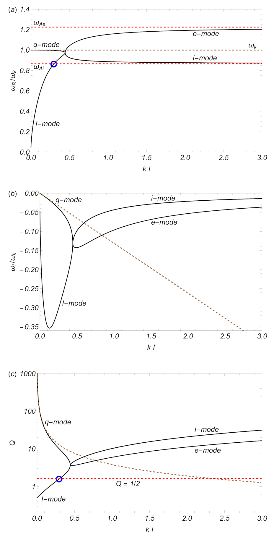
Figure 1a shows the real part of the frequency as a function of . When , one finds a solution with , as expected according to the analytic approximations and to be called the `q-mode’ after the `quasi-mode’. Unexpectedly, there is another solution that appears only when . The presence of this other solution was not predicted by the analytic approximations. The real part of the frequency of this additional solution grows from zero as l increases and, for this reason, it is labelled as the `l-mode’. Certainly, the l-mode owes its existence to the presence of the nonuniform transition. As increases, the q-mode and the l-mode eventually converge, and two different solutions or branches emerge afterwards. For the set of parameters used in Figure 1a, this happens around . The behaviour of of the two new branches is strikingly different. In the case of the lower branch, its tends to when . For this reason, the lower branch is labelled as the `i-mode’. Conversely, the real part of the frequency of the upper branch tends to when , so the upper branch is labelled as the `e-mode’. The q-mode, which is the descendent of the surface wave of the abrupt interface, ceases to exist as such when it collides with the l-mode and the i- and e-branches subsequently emerge. This suggests that an interface with a sufficiently thick transitional layer is not able to support a global collective mode. Below, more arguments in support of this idea are given.
To shed more light on the behaviour of the solutions, let us turn now to . Figure 1b displays as a function of . For the q-mode, the behaviour of when is again correctly described by the analytical formula for a thin transitional layer. Before the q-mode and the l-mode merge, it is found that the q-mode increases (in absolute value) with . The agreement between the approximate linear dependence with and the full result is good enough when .
On the other hand, the nature of the l-mode becomes even more puzzling when one realizes that it is a strongly attenuated solution. This fact can be better visualized in Figure 1c, which displays the quality factor, Q, of the solutions as a function of . The quality factor measures the efficiency of the damping and is defined as
Modes are overdamped when . An overdamped mode decays in a shorter timescale than its own period, which means that overdamped modes do not represent actual oscillations in the plasma but very short-lived motions. If a single period cannot be completed, the plasma motion can hardly be called an oscillation. Initially, the l-mode is heavily overdamped, and so it does not represent an actual oscillation. As increases, the l-mode quality factor increases until it crosses the critical value . It turns out that this happens, precisely, when the real part of the frequency of l-mode coincides with the lowest Alfvén frequency, i.e., , so that l-mode enters inside the Alfvén continuum (see the blue circles in panels a and c of Figure 1). From there on, and until it merges with the q-mode, the l-mode is another oscillatory solution that lives in the Alfvén continuum.
After q- and l-modes collide and the i- and e-modes subsequently emerge, the situation is as follows. The imaginary part of the frequencies of both the i- and e-modes decreases (in absolute value) and then tends to zero for . The quality factor of the e-mode is always smaller than that of the i-mode. Essentially, this is a consequence of the e-mode having a larger .
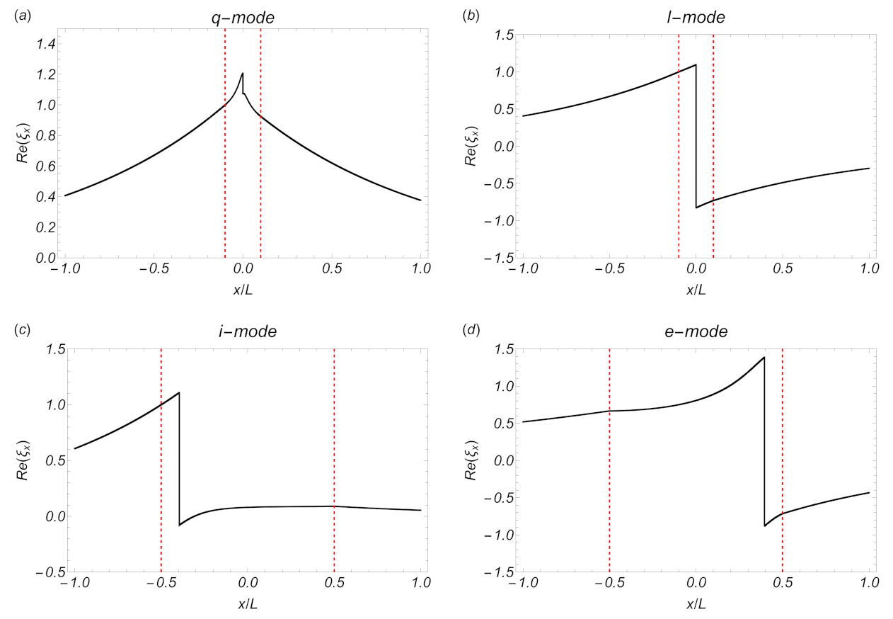
Although the physical interpretation of the q-mode is straightforward, it is the quasi-mode that descends from the undamped surface mode, and understanding the nature of the l-, i- and e-modes is more challenging. To further explore the nature of the solutions, Figure 2 displays the real part of their corresponding Lagrangian displacement, , in two cases, when and when . These two values of are chosen as representatives to the scenarios before and after the merging of the q- and l-modes. The solutions when are the q- and l-modes, while the solutions when are the i- and e-modes.
The perturbations of the q-mode when retain the shape expected from a surface wave, with the additional presence of the jump in due to the logarithmic Alfvénic singularity. The q-mode is an even (symmetric) mode as the surface wave for should necessarily satisfy the physical requirement that must be continuous at the abrupt interface. However, when , the hard requirement that must necessarily be an even function no longer applies. The two uniform plasmas may equally be connected through the nonuniform transition with either an even or an odd function. In principle, the two symmetries should be possible. The q-mode, being the descendant of the surface wave, retains the even symmetry. In turn, a new solution is introduced, the l-mode, whose is an odd (antisymmetric) function that jumps and changes sign at . Let us recall that l-mode is an overdamped solution for small and does not physically represent an oscillation. Only the q-mode represents an actual oscillation supported by a thin nonuniform interface.
Concerning the perturbations of the i- and e-modes when , the jumps in due to the resonances of these two modes in the Alfvén continuum are evident in Figure 2. The i-mode has a larger amplitude near the left boundary of the interface, while the e-mode has a larger amplitude near the right boundary. This result supports the idea that the two modes that split after the coalescence of the q- and l-modes are actually related with the uniform plasmas at each side of the interface and do not represent true collective modes of the whole interface. One can also see that the i-mode has inherited the even symmetry of the q-mode in the sense that the sign of is the same in the two plasmas at both sides of the interface, while the e-mode retains the odd symmetry of the l-mode; i.e., the sign of is the opposite in the two uniform plasmas.
4. Discussion
Despite the simplicity of the background model, the research discussed in this paper reveals interesting findings. While the ideal quasi-mode (q-mode) in a nonuniform interface has been explored in many works, almost all previous investigations were invariably restricted to the case of thin transitions. To the best of our knowledge, the results beyond the TB limit are unique in the sense that the existence of an additional solution with odd symmetry, the l-mode, has not been reported before in the literature. In the interface model, the l-mode owes its existence to the presence of the nonuniform region. However, although the l-mode is a solution of the dispersion relation, it should not be called a quasi-mode.
One can try to compare the results obtained here with those obtained in [15,29], that investigated not an interface, but a uniform slab with two nonuniform transitions at its sides. The results of [15] in the incompressible slab model can straightforwardly be related to the present findings (see Figure 2 in Ref. [15]). Ref. [15] also finds that the slab supports two different modes that have even (q-mode) and odd (l-mode) symmetries, respectively, although there is an important difference between the results of this study and those of [15]. In the case of the slab model of [15], modes with both even and odd symmetries are already geometrically possible in the absence of nonuniform transitions, while in the abrupt interface model, only a mode with even symmetry is possible. Hence, the peculiar behaviour of the l-mode in the interface model is related with the fact that an odd mode cannot exist for . In contrast, the results for thick transitions in both interface and slab models agree remarkably well. The `first solution’ in Ref. [15] corresponds to the i-mode, while their `second solution’ is equivalent to the e-mode. On the other hand, Ref. [29] considered the compressible case, and their results also show the presence of two surface-like solutions with even and odd symmetries. In addition, Ref. [29] found a third body-like solution with odd symmetry that is absent in the incompressible limit of [15]. Unfortunately, Ref. [29] did not explore the behaviour of their solutions with the thickness of the nonuniform layers, and a direct comparison of the present results with those of Ref. [29] is not possible.
In conclusion, it is found that when the width of the transition is thin, the ideal collective oscillations of the interface can be described by a quasi-mode that descends from the undamped surface mode of the equivalent abrupt interface, i.e., the q-mode. This solution lives on the Riemann sheet of the dispersion relation. This was already well known in the literature. In addition, there is another solution also present on the same Riemann sheet, the l-mode, which does not physically represent an oscillation because it is heavily overdamped. This other solution should not be called a quasi-mode. The existence of the l-mode merely reflects the possibility that the two uniform plasmas can be connected through the nonuniform transition with an odd function for , whereas the odd symmetry is forbidden when . If the transition is sufficiently thick, the q- and l-modes interact and eventually merge. Then, two new oscillatory modes, the i- and e-modes, appear. Although these new modes are not overdamped and have their frequencies in the Alfvén continuum, they do not truly represent global oscillations of the thick interface either. Instead, the shapes of their perturbations reveal that the i- and e-modes are associated with the uniform plasmas at both sides of the interface. Therefore, the coalescence of the q- and l-modes happens when the interface is not able to support a collective oscillation any more. Why this happens can be understood with an argument from [16]: if the nonuniform transition is so thick that the two uniform plasmas are far from each other, the transition can no longer be called an interface or a surface; if there is no surface, there can be no surface mode.
To conclude, let us note that the results obtained here pose a relevant theoretical problem that applies not only to the interface model but more generally to the study of ideal MHD oscillations in nonuniform plasmas: how to correctly interpret the zeros of the dispersion function found on a non-principal Riemann sheet. Should all the zeros equally be interpreted as quasi-modes that represent collective oscillations? In view of the present findings, we argue that extreme caution is needed and additional information such as, e.g., the spatial shape of the perturbations is required to draw meaningful conclusions about the nature of the solutions.
Funding
This publication is part of the R+D+i project PID2020-112791GB-I00, financed by MCIN/AEI/10.13039/501100011033.
Data Availability Statement
Not applicable.
Acknowledgments
The idea to carry out this theoretical investigation originated some time back, between 2010 and 2012, when the author was a postdoctoral researcher at the Centre for mathematical Plasma Astrophysics (CmPA) in Leuven, Belgium, under the supervision of Marcel Goossens. The idea was inspired by conversations with Marcel Goossens and other colleagues. Although some preliminary results were obtained back then, the work remained largely unfinished, and it was neither shared nor published. The research was resumed and expanded to contribute to this Special Issue on the occasion of Marcel Goossens’s 75th birthday. It is my sincere pleasure to dedicate this work to Marcel, from whom I have learnt so much during these years of fruitful collaboration.
Conflicts of Interest
The author declares no conflict of interest. The funders had no role in the design of the study; in the collection, analyses, or interpretation of data; in the writing of the manuscript; or in the decision to publish the results.
References
- Low, B.C. Field topologies in ideal and near-ideal magnetohydrodynamics and vortex dynamics. Sci. China Phys. Mech. Astron. 2015, 58, 015201. [Google Scholar] [CrossRef] [Green Version]
- Nakariakov, V.M.; Kolotkov, D.Y. Magnetohydrodynamic waves in the solar corona. Annu. Rev. Astron. Astrophys. 2020, 58, 441–481. [Google Scholar] [CrossRef]
- Wentzel, D.G. Hydromagnetic surface waves. Astrophys. J. 1979, 227, 319–322. [Google Scholar] [CrossRef]
- Roberts, B. Wave propagation in a magnetically structured atmosphere. I: Surface waves at a magnetic interface. Sol. Phys. 1981, 69, 27–38. [Google Scholar] [CrossRef]
- Goossens, M.; Andries, J.; Soler, R.; Van Doorsselaere, T.; Arregui, I.; Terradas, J. Surface Alfvén waves in solar flux tubes. Astrophys. J. 2012, 753, 111. [Google Scholar] [CrossRef] [Green Version]
- Sedláček, Z. Electrostatic oscillations in cold inhomogeneous plasma. I. Differential equation approach. J. Plasma Phys. 1971, 5, 239–263. [Google Scholar] [CrossRef]
- Rae, I.C.; Roberts, B. Surface waves and the heating of the corona. Geophys. Astrophys. Fluid Dyn. 1981, 18, 197–226. [Google Scholar] [CrossRef]
- Heyvaerts, J.; Priest, E.R. Coronal heating by phase-mixed shear Alfven waves. Astron. Astrophys. 1983, 117, 220–234. Available online: https://articles.adsabs.harvard.edu/pdf/1983A%26A...117..220H (accessed on 15 October 2022).
- Cally, P.S. Phase-mixing and surface waves: A new interpretation. J. Plasma Phys. 1991, 45, 453–479. [Google Scholar] [CrossRef]
- Soler, R.; Terradas, J. Magnetohydrodynamic kink waves in nonuniform solar flux tubes: Phase mixing and energy cascade to tmall scales. Astrophys. J. 2015, 803, 43. [Google Scholar] [CrossRef] [Green Version]
- Ionson, J.A. Resonant absorption of Alfvenic surface waves and the heating of solar coronal loops. Astrophys. J. 1978, 226, 650–673. [Google Scholar] [CrossRef]
- Abels-van Maanen, A.E.P.M.; Weenink, M.P.H. Collisionless damping of Alfvén waves in an inhomogeneous plasma: Solution of the initial value problem. Radio Sci. 1979, 14, 301–308. [Google Scholar] [CrossRef]
- Lee, M.A.; Roberts, B. On the behavior of hydromagnetic surface waves. Astrophys. J. 1986, 301, 430–439. [Google Scholar] [CrossRef]
- Hollweg, J.V. Resonant decay of global MHD modes at ’thick’ interfaces. J. Geophys. Res. 1990, 95, 2319–2324. [Google Scholar] [CrossRef]
- Tatsuno, T.; Wakatani, M. Damping of surface Alfvén wave in a slab plasma. J. Phys. Soc. Jpn. 1998, 67, 2322–2326. [Google Scholar] [CrossRef]
- Van Doorsselaere, T.; Poedts, S. Modifications to the resistive MHD spectrum due to changes in the equilibrium. Plasma Phys. Control. Fusion 2007, 49, 261–271. [Google Scholar] [CrossRef]
- Tataronis, J.; Grossmann, W. Decay of MHD waves by phase mixing. Z. Phys. A 1973, 261, 203–216. [Google Scholar] [CrossRef]
- Goossens, M.L.; Arregui, I.; Van Doorsselaere, T. Mixed properties of MHD waves in non-uniform plasmas. Front. Astron. Space Sci. 2019, 6, 20. [Google Scholar] [CrossRef]
- Sakurai, T.; Goossens, M.; Hollweg, J.V. Resonant behaviour of MHD waves on magnetic flux tubes. I. Connection formulae at the resonant surfaces. Sol. Phys. 1991, 133, 227–245. [Google Scholar] [CrossRef]
- Goossens, M.; Hollweg, J.V.; Sakurai, T. Resonant behaviour of MHD waves on magnetic flux tubes. III. Effect of equilibrium flow. Sol. Phys. 1992, 138, 233–255. [Google Scholar] [CrossRef]
- Soler, R.; Goossens, M.; Terradas, J.; Oliver, R. The behavior of transverse waves in nonuniform solar flux tubes. I. Comparison of ideal and resistive results. Astrophys. J. 2013, 777, 158. [Google Scholar] [CrossRef]
- Goedbloed, J.P.H.; Poedts, S. Principles of Magnetohydrodynamics; Cambridge University Press: Cambridge, UK, 2004. [Google Scholar] [CrossRef] [Green Version]
- Abramowitz, M.; Stegun, I.A. (Eds.) Handbook of Mathematical Functions with Formulas, Graphs, and Mathematical Tables; United States Department of Commerce, National Bureau of Standards: Washington, DC, USA, 1972; Available online: https://personal.math.ubc.ca/~cbm/aands/abramowitz_and_stegun.pdf (accessed on 15 October 2022).
- Goossens, M.; Erdélyi, R.; Ruderman, M.S. Resonant MHD waves in the solar atmosphere. Space Sci. Rev. 2011, 158, 289–338. [Google Scholar] [CrossRef]
- Edwin, P.M.; Roberts, B. Wave propagation in a magnetic cylinder. Sol. Phys. 1983, 88, 179–191. [Google Scholar] [CrossRef]
- Goossens, M.; Terradas, J.; Andries, J.; Arregui, I.; Ballester, J.L. On the nature of kink MHD waves in magnetic flux tubes. Astron. Astrophys. 2009, 503, 213–223. [Google Scholar] [CrossRef] [Green Version]
- Poedts, S.; Kerner, W. Ideal quasimodes reviewed in resistive magnetohydrodynamics. Phys. Rev. Lett. 1991, 66, 2871–2874. [Google Scholar] [CrossRef] [PubMed]
- Terradas, J.; Oliver, R.; Ballester, J.L. Damped coronal loop oscillations: Time-dependent results. Astrophys. J. 2006, 642, 533–540. [Google Scholar] [CrossRef] [Green Version]
- Arregui, I.; Terradas, J.; Oliver, R.; Ballester, J.L. Resonantly damped surface and body MHD waves in a solar coronal slab with oblique propagation. Sol. Phys. 2007, 246, 213–230. [Google Scholar] [CrossRef]
Figure 1.
Real part (a), imaginary part (b), and quality factor (c) of the solutions versus . The solid lines are the numerical results of the dispersion relation (Equation (17)), and the dashed brown lines are the analytic results for thin transitions (Equations (28) and (29)). The two horizontal dashed red lines in panel (a) denote and . The horizontal dashed red line in panel (c) denotes . The blue circles in panels (a,c) mark the entering of the l-mode in the Alfvén continuum. Frequencies are normalized to . , , and are used here, where L is a normalization length.

Figure 2.
Real part of (in arbitrary units) of the solutions: (a) q-mode for , (b) l-mode for , (c) i-mode for , and (d) e-mode for . The two vertical dashed red lines denote the boundaries of the nonuniform region. , , and are used here, where L is a normalization length. See text for details.
Figure 2.
Real part of (in arbitrary units) of the solutions: (a) q-mode for , (b) l-mode for , (c) i-mode for , and (d) e-mode for . The two vertical dashed red lines denote the boundaries of the nonuniform region. , , and are used here, where L is a normalization length. See text for details.

Publisher’s Note: MDPI stays neutral with regard to jurisdictional claims in published maps and institutional affiliations. |
© 2022 by the author. Licensee MDPI, Basel, Switzerland. This article is an open access article distributed under the terms and conditions of the Creative Commons Attribution (CC BY) license (https://creativecommons.org/licenses/by/4.0/).
Share and Cite
MDPI and ACS Style
Soler, R. Exploring the Ideal MHD Quasi-Modes of a Plasma Interface with a Thick Nonuniform Transition. Physics 2022, 4, 1359-1370. https://doi.org/10.3390/physics4040087
AMA Style
Soler R. Exploring the Ideal MHD Quasi-Modes of a Plasma Interface with a Thick Nonuniform Transition. Physics. 2022; 4(4):1359-1370. https://doi.org/10.3390/physics4040087
Chicago/Turabian StyleSoler, Roberto. 2022. "Exploring the Ideal MHD Quasi-Modes of a Plasma Interface with a Thick Nonuniform Transition" Physics 4, no. 4: 1359-1370. https://doi.org/10.3390/physics4040087