Abstract
This paper presents a two-qubit model derived from an SU(2)-symmetric 4×4 Hamiltonian. The resulting model is physically significant and, due to the SU(2) symmetry, is exactly solvable in both time-independent and time-dependent cases. Using the formal, general form of the related time evolution operator, the time dependence of the entanglement level for certain initial conditions is examined within the Rabi and Landau–Majorana–Stückelberg–Zener scenarios. The potential for applying this approach to higher-dimensional Hamiltonians to develop more complex exactly solvable models of interacting qubits is also highlighted.
1. Introduction
The two-level approximation, where the dynamics of a quantum system are limited to only two states, is commonly recognized for its broad applications in both physics and chemistry [1,2,3,4,5,6]. For instance, recent studies have demonstrated that the two-level formalism is effective in accurately describing the dynamics of charge transfer [7,8] and molecules in optical cavities [3]. Additionally, over the past few decades, the two-level quantum dynamical problem has become crucial in various quantum technologies, including quantum computing [9,10,11], quantum sensing [12,13], quantum information processing [14,15], and quantum metrology [16,17].
In quantum computing, beyond implementing qubits correctly, it is crucial to initialize and measure them with precision. This is where quantum control becomes essential. Quantum control Hamiltonians, which are time-dependent and characterized by external driving forces, are designed to manage qubit dynamics. Identifying exactly solvable single-qubit scenarios, where the time evolution operator of time-dependent Hamiltonians can be analytically derived, is crucial. Numerous mathematical approaches have been developed to tackle exactly solvable two-level dynamical problems [18,19,20,21,22,23,24,25], given the general difficulty of solving the Schrödinger equation with a time-dependent Hamiltonian. Among these, the Rabi [26] and Landau–Majorana– Stückelberg–Zener (LMSZ) [27,28,29,30,31] scenarios are particularly notable for their extensive applications in physics. This research is broadly relevant, as analytical solutions for single two-level systems have been helpful in more complex systems without spin variables [32], and similar approaches have been used to solve non-Hermitian two-level dynamical problems [33].
In many-qubit scenarios, however, the coupling between different effective two-level systems (TLSs) cannot be ignored [34,35]. In contexts like quantum computation, tuning the interaction between TLSs is essential for using quantum logic gates that generate entangled states witha high level of entanglement [36,37,38], which is a key resource in quantum computation [39]. Investigating more complex models comprising many interacting qubits, which can be analytically treated to obtain exact results, is then relevant as well. For this reason, significant attention has been given to the simplest many-qubit system: the two-qubit scenario. This involves two TLSs interacting either directly (through exchange, Heisenberg, and Dzialoshinskii–Moriya (DM) interactions) or indirectly (via photon-mediated interaction). This focus is evidenced by the extensive research on quantum gates and operational protocols in two-qubit systems across various platforms [40,41,42,43,44,45,46,47,48,49,50,51,52,53,54,55,56,57,58].
Developing strategies to solve the dynamical problem of two-qubit time-dependent Hamiltonians, in order to fully control the dynamics of two interacting qubits, is also crucial. For example, in Ref. [59], the original two-qubit problem is decomposed into two independent single-qubit subproblems related to two dynamically invariant subspaces, thanks to a specific Hamiltonian symmetry and its constant of motion. Thus, by leveraging exact solutions for single-qubit scenarios, exact solutions for the two-qubit problem have been derived, revealing physical effects in both closed [60,61,62] and open [63] systems.
Nevertheless, other exactly solvable and analytically treatable two-qubit models, presenting no constants of motion, can exist. This paper presents a general time-dependent two-qubit Hamiltonian model without integrals of motion, whose time evolution operator can still be formally expressed and, in specific cases, analytically derived. This study utilizes group theory particularly focusing on the SU(2) group. By exactly solving the dynamical problem, this paper investigates the exact time dependence of the concurrence (which measures the level of entanglement between the two qubits) in three scenarios: time-independent, Rabi, and LMSZ. It is demonstrated how the controlled generation of entanglement is achievable both periodically and asymptotically in adiabatic and non-adiabatic regimes. Finally, it is particularly significant that the method demonstrated in this paper for two-qubit systems can be similarly applied to higher-dimensional Hamiltonians. Therefore, this approach allows for the development of exactly solvable Hamiltonian models that describe the dynamics of more complex systems involving multiple interacting qubits or, more generally, qudits.
The paper is structured as follows. Section 2 introduces the basics of the SU(2) symmetry group and derives the new two-qubit Hamiltonian model. Section 3 discusses three possible solutions to the dynamical problem, while Section 4 examines the time behavior of the two-qubit concurrence. Finally, Section 5 provides concluding remarks.
2. The Model
2.1. SU(2) Symmetry
The SU(2)-symmetric group is a compact group whose lowest-dimensional matrix representation consists of the set of all two-dimensional unitary matrices of the form
with a and b being two complex parameters satisfying . The generators of this 2×2 representation of the SU(2) group are the Pauli matrices: , , and . The most general generator, a combination of the three Pauli matrices, can then be written as
with and denoting, respectively, the magnitudes of the transverse and the longitudinal fields on the spin, and the matrix is represented in the basis of . It is worth underlining that values are the generators of in the sense that values are the solutions of the equation (where the dot denotes the time derivative), which is nothing but the Schrödinger (with the reduced Planck constant ) equation for a physical system described by the Hamiltonian H. This holds when the Hamiltonian is both time-dependent and time-independent (the time plays the role of the group parameter). In the time-independent case, the expressions of a and b can be straightforwardly derived by diagonalizing the Hamiltonian. In the time-dependent case of H, instead, the solution of the system for a and b, stemming from the Schrödinger equation, can be quite a complicated task. However, several examples of exactly solvable dynamical problems related to time-dependent Hamiltonians exist [18,19,20,21,22,23,24,25,26,27,31,59].
Matrix representations of the same SU(2) group in higher dimensions are also possible. The three-dimensional representation, for example, consists of all 3×3 unitary matrices whose generators are linear combinations of the three spin-1 Pauli matrices. The peculiarity at the basis of all representations is that they are always characterized by two independent parameters. That is, one can formally write the entries of the higher-dimensional unitary matrices of SU(2) as specific combinations of the two parameters a and b. The three-dimensional matrices, e.g., can be cast as
As far as physical problems are concerned, this aspect is highly relevant from a dynamical point of view, since it implies that high-dimensional SU(2)-symmetric dynamical problems can be solved by solving the related analogous 2×2 SU(2) dynamical problem.
In this study, the 4×4 representation of the SU(2) group is considered. The 4×4 unitary matrices constituting the set read
The related generators are the spin-3/2 operators and the most general linear combination, in the basis of , is
Also, in this case, apparently, the matrix is the formal solution of the equation . Certainly, depending on the forms of and (in the general time-dependent case), one obtains different expressions of a and b, solutions of the two independent equations stemming from the Schrödinger equation.
2.2. SU(2) Two-Qubit Model
One can interpret , which is the 4×4 matrix representation of the generic generator of the SU(2) group, in terms of two spin-qubits. In other words, one can interpret the Hamiltonian as written in the composite basis of the two qubits , with . It is possible to verify that the resulting two-qubit model reads
This describes two qubits interacting through a Heisenberg term depending on and a DM term [64,65] characterized by the DM vector (since the DM interaction is commonly written as [66], with , ). The first qubit is subjected to a magnetic field along the z direction, namely , while the second one is subjected to a different magnetic field with nonvanishing components on the three directions, precisely . Appendix A shows the Derivation of the SU(2) two-qubit model. One can see that, in order to obtain the SU(2) form, specific relations between the parameters of the two-qubit Hamiltonian exist. In particular, nterstingly, the link between the strength of the magnetic field on the x–y plane (on the second spin) and the interaction parameters, as well as the z-magnetic field on the first spin, which doubles the one on the second spin. To stress is that the magnetic fields written before, compared to the terms in the Hamiltonian, lack a factor since the Hamiltonian terms describe the coupling between the magnetic field and the spin magnetic moment, which, for a spin-1/2, is characterized by a pre-factor () in front of the Pauli matrices, namely, .
As discussed above, the dynamical problem related to such a two-qubit model can be solved by finding the solutions of a and b that can be derived by solving the analogous two-dimensional dynamical problem. Below three dynamical scenarios are considered.
3. Dynamical Scenarios
3.1. Time-Independent Case
First, consider the case where the three Hamiltonian parameters are time-independent, namely , (where , and ). In this case, one can talk about eigenenergies of the system, and they read
The expressions of a and b can be analytically derived and it is possible to verify that they result in
One can see that the parameter does not play any role in the dynamics since it does not appear in the above expressions of a and b. This finding is physically reasonable since the Hamiltonian can be unitarily transformed by performing a rotation in the x–y plane in order to obtain , that is, and .
3.2. Rabi Scenario
The Rabi scenario is characterized by a precessing magnetic field with a constant component along the z-axis and a rotating field on the x–y plane, that is,
where is the precession frequency of the field. In this case, a and b obtain the following expressions [26]:
with being the detuning and the Rabi frequency. corresponds to the known resonance condition for which the Rabi oscillations of the populations in a two-level system are characterized by the maximum amplitude [26]. It is worth stressing that the realization of a Rabi scenario for the two-qubit model under scrutiny could be challenging from an experimental point of view since the transverse magnetic field on the second spin and the coupling between the two qubits must be varied accordingly in order to maintain the SU(2) symmetry of the Hamiltonian. However, through trapped ion and superconducting circuit technologies, both parameters can be appropriately managed [67].
3.3. Landau–Majorana-Stückelberg–Zener Scenario
The LMSZ scenario [27,31] is characterized by a constant transverse field, i.e., , and a longitudinal ramp, that is, a linearly varying magnetic field along the z direction, namely (with the being the slope of the ramp), from negative to positive infinite values []. To consider negative values of time is a mathematical trick to formally describe the experimental procedure consisting of the inversion of the magnetic field. Precisely, the passage from negative to positive values means that the magnetic field is initially set along a specific direction and its modulus is linearly decreased in time until it vanishes. At this point, the modulus starts to be linearly increased in the opposite direction from the original one. The instant when the field vanishes is then the inversion point.
The related dynamical problem cannot be solved in general but only for specific initial states [27,31]. Moreover, it is not physically meaningful, from both a theoretical and experimental point of view, since an infinite field implies infinite energies, as well as an infinite process. However, the dynamical problem related to a ‘finite’ LMSZ scenario, that is, a ramp starting and ending at finite instants; i.e., , can be generally solved as well [68]. The expressions of a and b, although complicated, can be analytically derived and read [68]:
where , is the gamma function, is the parabolic cylinder functions [69], and is a time dimensionless parameter (let us stress that since , then ); and identifies the initial time instant. It is worth stressing that in this case, one can consider also non-symmetric time windows, that is, ; it is particularly relevant in the case with [68], which can generate entangled states of two-qubit [60] and two-qutrit [70] systems through an adiabatic change in the field ().
3.4. Two-Qubit Spin–Flip and Phase Gate Realization
In this Section, the possibility of performing two-qubit operation through the interaction model under scrutiny is outlined. It can be noted indeed that if considerably large times are considered in the LMSZ, that is, , one obtains and . In this instance, the time evolution operator acquires the following quite a simple form:
To note is that the same unitary matrix can be periodically generated in the Rabi scenario by putting for the time instants .
The operator (12) acts as a two-qubit spin–flip gate. The two-qubit standard basis states are indeed transformed as follows:
upon a physically not relevant global phase in the second and fourth case. Here, + and − denote the eigenstates of (namely, ). Such a phase factor, however, becomes crucial when superposition states are considered. This unitary operator indeed has the property of transforming the ‘analogous’ Bell states (that is, the Bell states obtained by the superposition of the same standard basis states) into each other, namely,
where and . On the basis of this property, it follows that such a unitary matrix transforms the ‘analogous’ Werner states into each other, the latter being written as
where is a real number in . Therefore, it means that through the interaction model derived here, one can accurately manipulate the Bell states of the two qubits with no loss in entanglement, by applying either a Rabi or a LMSZ magnetic field, which are the most experimentally feasible and employed fields.
4. Concurrence Dynamics
The level of entanglement of a two-qubit system can be quantified through the concurrence [71], which, in the case of a generic normalized pure state , acquires the following analytical form:
In Figure 1 and Figure 2 the concurrence is calculated for different initial conditions, namely when the two-qubit system is initialized in the state , , and (in each of Figure 1 and Figure 2a–c, respectively) for the time-independent (Rabi) scenario. One can see that the behavior of the concurrence is qualitatively similar in the two cases. This is due to the feature that the expressions of a and b for the Rabi scenario closely resemble the ones related to the time-independent case. This circumstance stems from the finding that the Rabi Hamiltonian can be unitarily transformed to a time-independent one by changing the reference frame from the laboratory one to the frame rotating with the precessing magnetic field. The time behaviors of the concurrence practically consist of periodic oscillations. It can be noted that Figure 1a and Figure 2a are identical, since, in that case, that is, for the initial condition , the concurrence results to be . In this instance, the factor , appearing in the expressions of a and b for the Rabi scenario, does not play any role, contrary to what occurs in the other cases (Figure 1b,c and Figure 2b,c), which show slight differences.
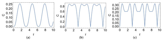
Figure 1.
Time dependence of the concurrence for the initial condition: (a) , (b) , and (c) , in the time-independent case when as a function of the dimensionless time . See text for details.

Figure 2.
Time dependence of the concurrence for the initial condition: (a) , (b) , and (c) , in the Rabi scenario when as a function of the dimensionless time . See text for details.
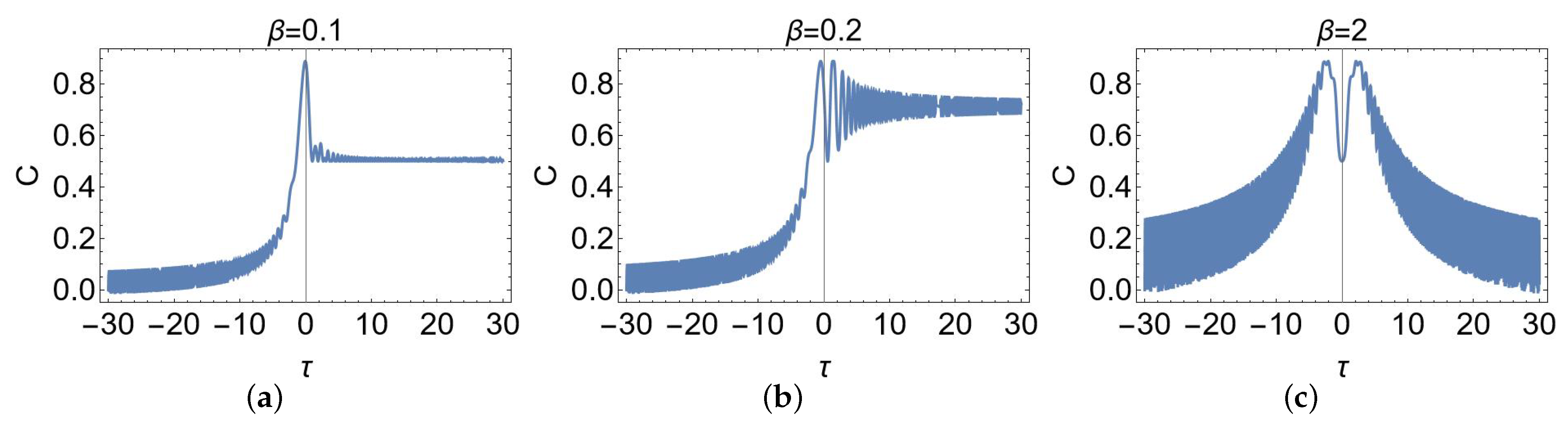
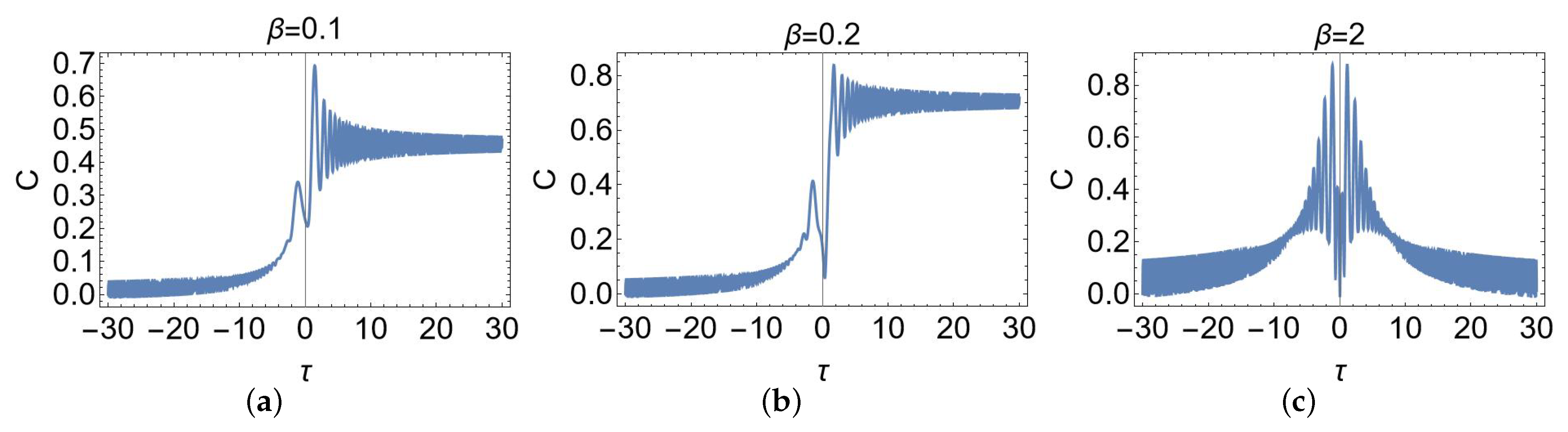
In Figure 3, Figure 4 and Figure 5, the time behavior of the concurrence in the LMSZ scenario is plotted for the three initial conditions , , and , respectively. The value of determines the level of adiabaticity of the dynamics. In particular, for (), the system is driven by a non-adiabatic (adiabatic) process.
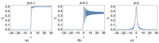
Figure 3.
Time dependence of the concurrence in the LMSZ scenario, as a function of the dimensionless time , for the initial condition , when (a) , (b) , (c) . See text for details.

Figure 4.
Time dependence of the concurrence in the LMSZ scenario, as a function of the dimensionless time , for the initial condition , when (a) , (b) , (c) . See text for details.
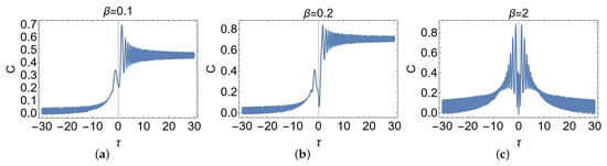
Figure 5.
Time dependence of the concurrence in the LMSZ scenario, as a function of the dimensionless time , for the initial condition , when (a) , (b) , (c) . See text for details.
The differences between the cases related to and in Figure 3, Figure 4 and Figure 5 are only quantitative. The system indeed starts from a vanishing concurrence (since the considered initial conditions are separable); then, after the inversion of the field, an amount of entanglement is generated between the two qubits.
A qualitatively different behavior is instead obtained for the plots with . In this case, for the three initial conditions, the maximum level of entanglement is generated at or near the central point (the inversion point of the field). At considerably large times, the concurrence tends to zero again, meaning that the system comes back to a separable state. This can be seen by explicitly writing the evolved states at time t, obtaining
and by taking into account that, for adiabatic dynamics, () and . In this limit, it is possible to see that , , and obtain a separable form, namely
justifying the vanishing concurrence at quite large times. Let us note that this kind of dynamics practically consist of full state inversion, that is, in flipping the spin states. Contrarily, for non-adiabatic dynamics (), the state at considerably large times is not separable, presenting a non-vanishing level of entanglement.
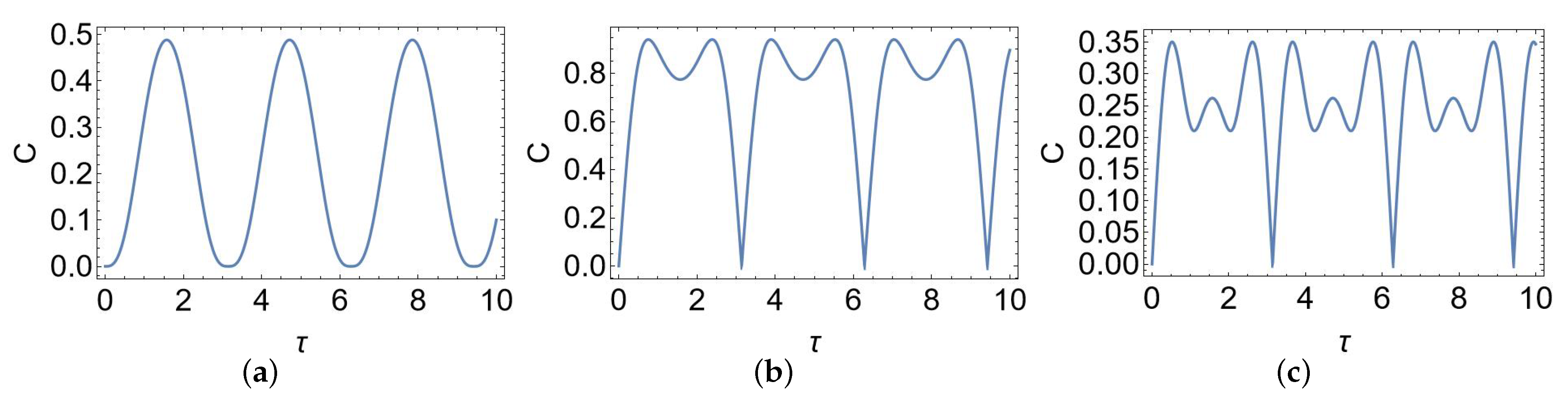
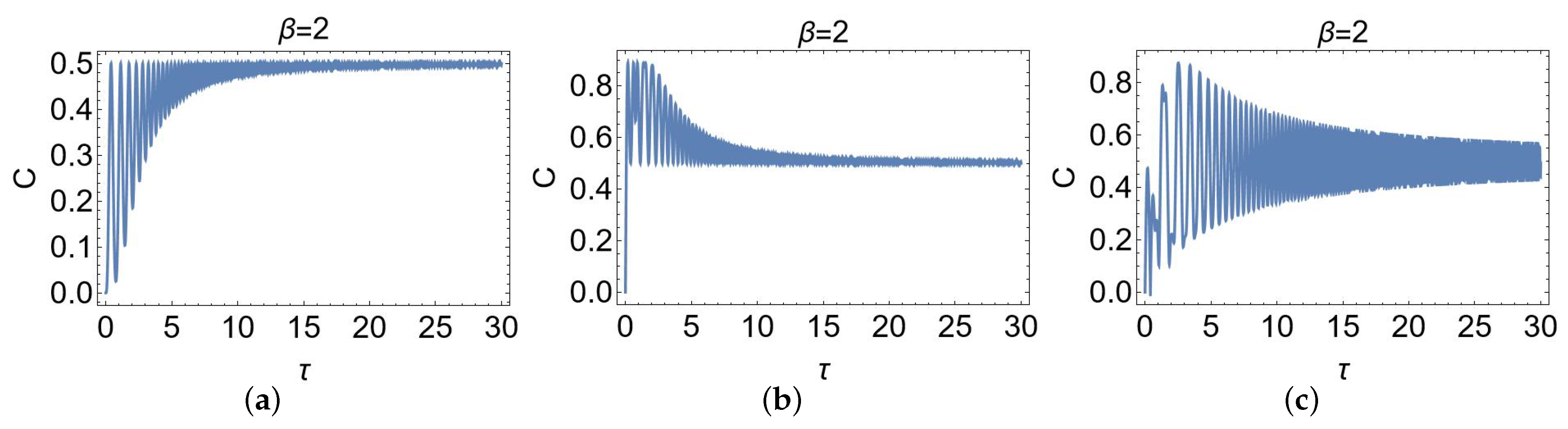
However, it is instructive to show that it is also possible to generate entanglement also through adiabatic dynamics. In this case, it is sufficient to modify the procedure of application of the magnetic field; namely, it serves only to modify the time window, leaving the linear time dependence of the ramp unchanged. Indeed, for a half ramp, that is, a magnetic field initially vanishing and then linearly increasing, the production of of entanglement can be seen in Figure 6. One can see that in the three cases, the concurrence, starting from a vanishing value, asymptotically tends to a (almost) constant value, namely . In the transient, for the cases in subplots Figure 6b,c, a high level of entanglement, corresponding to , is reached by the two-qubit system during the adiabatic dynamics.

Figure 6.
Time dependence of the concurrence in the LMSZ scenario as a function of the dimensionless time , for the initial condition: (a) , (b) , and (c) and for adiabatic procedures, namely when . See text for details.
Finally, it is worth stressing that the fast oscillations clearly visible in all of the plots related to the LMSZ scenario are not due to approximations adopted to obtain the plots. Rather, they are related to the fast oscillating cylinder functions appearing in the analytical solutions of the LMSZ model given in Equation (11).
5. Conclusions
In this paper a model of two interacting qubits has been presented and studied. Special emphasis has been placed on the method used to obtain the model. The model has indeed been derived by first considering the finite four-dimensional representation of the general generator of the SU(2) group. This 4×4 matrix can be expressed in operator form using spin-3/2 Pauli operators, resulting in a single spin-3/2 (a four-level system) subjected to a magnetic field with generally non-zero components in three independent directions.
However, this same 4×4 matrix can also be interpreted in terms of the Pauli matrices of two spin-1/2 particles (TLSs or qubits). By translating it into the language of two TLSs, a model of two qubits interacting through both exchange and Dzialoshinskii–Moriya interaction terms is obtained. These two qubits are also subjected to different local magnetic fields: the first qubit experiences only a longitudinal (z) magnetic field, while the second is subjected to both longitudinal and transverse (x–y plane) magnetic fields. To maintain the SU(2) symmetry of the generator, specific relations exist between the Hamiltonian parameters, such as the longitudinal magnetic field on the first qubit being twice that on the second qubit, and the coupling strength of interaction parameters being closely related to the transverse magnetic field magnitude on the second qubit.
The significance of an SU(2)-symmetric model lies in the understanding of the general structure of the operator U generated by the Hamiltonian H through (). In physical terms, U is the time evolution operator. The general structure of U, dependent on two generally complex parameters (which can be found by solving the related Schrödinger equation), holds for both time-dependent and time-independent Hamiltonian parameters. While the time-independent case is straightforwardly solvable, the time-dependent one depends on the specific time dependence of the field, making exact solutions generally challenging to find. However, thanks to the SU(2) symmetry, one can derive exact solutions for the two-qubit problem from known solutions of single-qubit dynamical problems. This considerably simplifies the task since numerous exactly solvable single-qubit scenarios (with analytical solutions to the Schrödinger equation) exist in the literature [18,19,20,21,22,23,24,25,26,27,28,29,30,31,59]. Consequently, one can derive the exact dynamics of the two qubits for all these scenarios. This means one can fully control the evolution of the two-qubit system for these scenarios and apply specific applications developed for single two-level systems [72,73,74,75,76,77] to two-qubit scenarios. To stress is that the same considerations also hold when higher-dimensional Hamiltonians are considered. This situation highlights the method’s potential applicability and its physical significance for use in many-qubit scenarios.
Beyond the time-independent case, the paper considered the most known exactly solvable time-dependent scenarios: the Rabi and LMSZ scenarios. The exact expressions of the two parameters defining the time evolution operator have allowed us to derive the analytical form of the evolved states from certain initial (separable) conditions. In particular, the time evolution of concurrence, a measure of the entanglement between the two qubits, have been analyzed. High levels of entanglement can be generated through such interaction models and scenarios. Additionally, it has been highlighted how, in the LMSZ scenario, high concurrence values can be generated differently depending on the procedure’s adiabaticity level (i.e., the slope of the magnetic field).
Finally, it is worth underlining that the potential of the method used to obtain the SU(2)-symmetric two-qubit model lies in its applicability to more complex Hamiltonians and physical scenarios. For instance, applying this procedure to a 6×6, 8×8, or 9×9 SU(2)-symmetric matrix yields exactly solvable models for qubit–qutrit, three-qubit, and two-qutrit systems, respectively. In these cases, the method thus allows for the appropriate control of more complex physical systems’ quantum dynamics with consequent possible advantages for quantum computation tasks.
Funding
The author acknowledges financial support from the PNRR MUR (Progetto Nazionale di Ripresa e Resilienza-Ministero dell’Universitá e della Ricerca) project PE0000023-NQSTI (National Quantum Science and Technology Institute), Italy.
Data Availability Statement
The original contributions presented in the study are included in the article.
Acknowledgments
The author warmly thanks Antonino Messina for fruitful discussions.
Conflicts of Interest
The author declares no conflicts of interest.
Appendix A. Derivation of the SU(2) Two-Qubit Model
This Appendix outlines the technical details on the basis of the derivation of the two-qubit model in Section 2. As declared in this paper, one can write the operator form of the 4×4 SU(2) matrix in Equation (5) in terms of the Pauli operators of two qubits.
To begin with, it is instructive to express the entries of a 2×2 matrix in terms of the Pauli operators as follows:
Certainly, the entries of a 4×4 matrix in terms of two-qubit Pauli operators can be written as tensor product of the single-qubit operators, for example,
In this way, by expressing the the appropriate operator form of each entry of the 4×4 SU(2) matrix and summing the analogous term, one can derive the expression of the Hamiltonian in Equation (6). The analogous procedure can be applied in the case of higher SU(2) Hamiltonians. For a 3×3 matrix, for example, the tensor product of the Pauli operators of three qubits must be employed.
References
- Dell’Anno, F.; De Siena, S.; Illuminati, F. Multiphoton quantum optics and quantum state engineering. Phys. Rep. 2006, 428, 53–168. [Google Scholar] [CrossRef]
- Shevchenko, S.; Ashhab, S.; Nori, F. Landau–Zener–Stückelberg interferometry. Phys. Rep. 2010, 492, 1–30. [Google Scholar] [CrossRef]
- Ivakhnenko, O.V.; Shevchenko, S.N.; Nori, F. Nonadiabatic Landau–Zener–Stückelberg–Majorana transitions, dynamics, and interference. Phys. Rep. 2023, 995, 1–89. [Google Scholar] [CrossRef]
- Newton, M.D. Quantum chemical probes of electron-transfer kinetics: The nature of donor-acceptor interactions. Chem. Rev. 1991, 91, 767–792. [Google Scholar] [CrossRef]
- Gupta, S.; Yang, J.H.; Yakobson, B.I. Two-level quantum systems in two-dimensional materials for single photon emission. Nano Lett. 2018, 19, 408–414. [Google Scholar] [CrossRef] [PubMed]
- Wang, D.; Kelkar, H.; Martin-Cano, D.; Rattenbacher, D.; Shkarin, A.; Utikal, T.; Götzinger, S.; Sandoghdar, V. Turning a molecule into a coherent two-level quantum system. Nat. Phys. 2019, 15, 483–489. [Google Scholar]
- Migliore, A. Nonorthogonality problem and effective electronic coupling calculation: Application to charge transfer in π-stacks relevant to biochemistry and molecular electronics. J. Chem. Theo. Comput. 2011, 7, 1712–1725. [Google Scholar] [CrossRef] [PubMed]
- Migliore, A.; Messina, A. Controlling the charge-transfer dynamics of two-level systems around avoided crossings. J. Chem. Phys. 2024, 160, 084112. [Google Scholar] [CrossRef]
- McArdle, S.; Endo, S.; Aspuru-Guzik, A.; Benjamin, S.C.; Yuan, X. Quantum computational chemistry. Rev. Mod. Phys. 2020, 92, 015003. [Google Scholar] [CrossRef]
- Koch, C.P.; Boscain, U.; Calarco, T.; Dirr, G.; Filipp, S.; Glaser, S.J.; Kosloff, R.; Montangero, S.; Schulte-Herbrüggen, T.; Sugny, D.; et al. Quantum optimal control in quantum technologies. Strategic report on current status, visions and goals for research in Europe. EPJ Quant. Technol. 2022, 9, 19. [Google Scholar] [CrossRef]
- Chiavazzo, S.; Sørensen, A.S.; Kyriienko, O.; Dellantonio, L. Quantum manipulation of a two-level mechanical system. Quantum 2023, 7, 943. [Google Scholar] [CrossRef]
- Chu, Y.; Liu, Y.; Liu, H.; Cai, J. Quantum sensing with a single-qubit pseudo-Hermitian system. Phys. Rev. Lett. 2020, 124, 020501. [Google Scholar] [CrossRef]
- Hönigl-Decrinis, T.; Shaikhaidarov, R.; de Graaf, S.; Antonov, V.; Astafiev, O. Two-level system as a quantum sensor for absolute calibration of power. Phys. Rev. Appl. 2020, 13, 024066. [Google Scholar] [CrossRef]
- Jafarizadeh, M.; Naghdi, F.; Bazrafkan, M. Time optimal control of two-level quantum systems. Phys. Lett. A 2020, 384, 126743. [Google Scholar] [CrossRef]
- Feng, T.; Xu, Q.; Zhou, L.; Luo, M.; Zhang, W.; Zhou, X. Quantum information transfer between a two-level and a four-level quantum systems. Photonics Res. 2022, 10, 2854–2865. [Google Scholar] [CrossRef]
- Yang, Y.; Liu, X.; Wang, J.; Jing, J. Quantum metrology of phase for accelerated two-level atom coupled with electromagnetic field with and without boundary. Quant. Inf. Process. 2018, 17, 54. [Google Scholar] [CrossRef]
- Pezzè, L.; Smerzi, A.; Oberthaler, M.K.; Schmied, R.; Treutlein, P. Quantum metrology with nonclassical states of atomic ensembles. Rev. Mod. Phys. 2018, 90, 035005. [Google Scholar] [CrossRef]
- Bagrov, V.G.; Gitman, D.M.; Baldiotti, M.C.; Levin, A.D. Spin equation and its solutions. Ann. Phys. 2005, 517, 764–789. [Google Scholar] [CrossRef]
- Kuna, M.; Naudts, J. General solutions of quantum mechanical equations of motion with time-dependent hamiltonians: A lie algebraic approach. Rep. Math. Phys. 2010, 65, 77–108. [Google Scholar] [CrossRef]
- Barnes, E.; Sarma, S.D. Analytically solvable driven time-dependent two-level quantum systems. Phys. Rev. Lett. 2012, 109, 060401. [Google Scholar] [CrossRef]
- Messina, A.; Nakazato, H. Analytically solvable Hamiltonians for quantum two-level systems and their dynamics. J. Phys. A Math. Theor. 2014, 47, 445302. [Google Scholar] [CrossRef]
- Markovich, L.; Grimaudo, R.; Messina, A.; Nakazato, H. An example of interplay between physics and mathematics: Exact resolution of a new class of Riccati equations. Ann. Phys. 2017, 385, 522–531. [Google Scholar] [CrossRef]
- Liang, H. Generating arbitrary analytically solvable two-level systems. J. Phys. A Math. Theor. 2024, 57, 095301. [Google Scholar] [CrossRef]
- Castaños, L. Simple, analytic solutions of the semiclassical Rabi model. Opt. Commun. 2019, 430, 176–188. [Google Scholar] [CrossRef]
- Castaños, L. A simple, analytic solution of the semiclassical Rabi model in the red-detuned regime. Phys. Lett. A 2019, 383, 1997–2003. [Google Scholar] [CrossRef]
- Rabi, I.I. Space quantization in a gyrating magnetic field. Phys. Rev. 1937, 51, 652–654. [Google Scholar] [CrossRef]
- Landau, L.D. A theory of energy transfer II. Phys. Z. Sowjetun. 1932, 2, 46–51, Reprinted in Collected Papers of L.D. Landau; Ter Haar, D., Ed.; Pergamon Press Ltd.: Oxford, UK; Gordon and Breach, Science Publishers Inc.: New York, NY, USA, 1965; pp. 63–66. [Google Scholar] [CrossRef]
- Majorana, E. Atomi orientati in campo magnetico variabile. Nuovo Cim. 1932, 9, 43–50. [Google Scholar] [CrossRef]
- Stückelberg, E.C.G. Theorie der unelastischen Stösse zwischen Atomen. Helv. Phys. Acta 1932, 5, 369–422. Available online: https://www.e-periodica.ch/digbib/view?pid=hpa-001%3A1932%3A5%3A%3A5#373 (accessed on 10 August 2024).
- Stückelberg, E.C.G. Theory of Inelastic Collisions between Atoms; Report NASA TT F-13,970; National Aerounatics Space Administration: Washington, DC, USA, 1971; Available online: https://archive.org/details/nasa_techdoc_19720003957 (accessed on 10 August 2024).
- Zener, C. Non-adiabatic crossing of energy levels. Proc. R. Soc. London. A Math. Phys. Engin. Sci. 1932, 137, 696–702. [Google Scholar] [CrossRef]
- Grimaudo, R.; Man’ko, V.I.; Man’ko, M.A.; Messina, A. Dynamics of a harmonic oscillator coupled with a Glauber amplifier. Phys. Scr. 2019, 95, 024004. [Google Scholar] [CrossRef]
- Grimaudo, R.; de Castro, A.S.M.; Nakazato, H.; Messina, A. Analytically solvable 2×2 PT-symmetry dynamics from su(1,1)-symmetry problems. Phys. Rev. A 2019, 99, 052103. [Google Scholar] [CrossRef]
- Calvo, R.; Abud, J.E.; Sartoris, R.P.; Santana, R.C. Collapse of the EPR fine structure of a one-dimensional array of weakly interacting binuclear units: A dimensional quantum phase transition. Phys. Rev. B 2011, 84, 104433. [Google Scholar] [CrossRef]
- Napolitano, L.M.B.; Nascimento, O.R.; Cabaleiro, S.; Castro, J.; Calvo, R. Isotropic and anisotropic spin-spin interactions and a quantum phase transition in a dinuclear Cu(II) compound. Phys. Rev. B 2008, 77, 214423. [Google Scholar] [CrossRef]
- Kang, Y.-H.; Chen, Y.-H.; Wu, Q.-C.; Huang, B.-H.; Song, J.; Xia, Y. Fast generation of W states of superconducting qubits with multiple Schrödinger dynamics. Sci. Rep. 2016, 6, 36737. [Google Scholar] [CrossRef]
- Lu, M.; Xia, Y.; Song, J.; An, N.B. Generation of N-atom W-class states in spatially separated cavities. J. Opt. Soc. Am. B 2013, 30, 2142–2147. [Google Scholar] [CrossRef]
- Li, J.; Paraoanu, G.S. Generation and propagation of entanglement in driven coupled-qubit systems. New J. Phys. 2009, 11, 113020. [Google Scholar] [CrossRef]
- Amico, L.; Fazio, R.; Osterloh, A.; Vedral, V. Entanglement in many-body systems. Rev. Mod. Phys. 2008, 80, 517–576. [Google Scholar] [CrossRef]
- Morzhin, O.V.; Pechen, A.N. Optimal state manipulation for a two-qubit system driven by coherent and incoherent controls. Quant. Inf. Process. 2023, 22, 241. [Google Scholar] [CrossRef]
- Ding, L.; Hays, M.; Sung, Y.; Kannan, B.; An, J.; Di Paolo, A.; Karamlou, A.H.; Hazard, T.M.; Azar, K.; Kim, D.K.; et al. High-fidelity, frequency-flexible two-qubit fluxonium gates with a transmon coupler. Phys. Rev. X 2023, 13, 031035. [Google Scholar] [CrossRef]
- Schäfter, D.; Wischnat, J.; Tesi, L.; De Sousa, J.A.; Little, E.; McGuire, J.; Mas-Torrent, M.; Rovira, C.; Veciana, J.; Tuna, F.; et al. Molecular one-and two-qubit systems with very long coherence times. Adv. Mater. 2023, 35, 2302114. [Google Scholar] [CrossRef] [PubMed]
- Mills, A.R.; Guinn, C.R.; Gullans, M.J.; Sigillito, A.J.; Feldman, M.M.; Nielsen, E.; Petta, J.R. Two-qubit silicon quantum processor with operation fidelity exceeding 99%. Sci. Adv. 2022, 8, eabn5130. [Google Scholar] [CrossRef]
- Petit, L.; Russ, M.; Eenink, G.H.; Lawrie, W.I.; Clarke, J.S.; Vandersypen, L.M.; Veldhorst, M. Design and integration of single-qubit rotations and two-qubit gates in silicon above one kelvin. Commun. Mater. 2022, 3, 82. [Google Scholar] [CrossRef]
- Noiri, A.; Takeda, K.; Nakajima, T.; Kobayashi, T.; Sammak, A.; Scappucci, G.; Tarucha, S. A shuttling-based two-qubit logic gate for linking distant silicon quantum processors. Nat. Commun. 2022, 13, 5740. [Google Scholar] [CrossRef] [PubMed]
- Moskalenko, I.N.; Simakov, I.A.; Abramov, N.N.; Grigorev, A.A.; Moskalev, D.O.; Pishchimova, A.A.; Smirnov, N.S.; Zikiy, E.V.; Rodionov, I.A.; Besedin, I.S. High fidelity two-qubit gates on fluxoniums using a tunable coupler. NPJ Quant. Inf. 2022, 8, 130. [Google Scholar] [CrossRef]
- Bresque, L.; Camati, P.A.; Rogers, S.; Murch, K.; Jordan, A.N.; Auffèves, A. Two-qubit engine fueled by entanglement and local measurements. Phys. Rev. Lett. 2021, 126, 120605. [Google Scholar] [CrossRef]
- Cai, T.Q.; Han, X.Y.; Wu, Y.K.; Ma, Y.L.; Wang, J.H.; Wang, Z.L.; Zhang, H.Y.; Wang, H.Y.; Song, Y.P.; Duan, L.M. Impact of spectators on a two-qubit gate in a tunable coupling superconducting circuit. Phys. Rev. Lett. 2021, 127, 060505. [Google Scholar] [CrossRef]
- Blümel, R.; Grzesiak, N.; Nguyen, N.H.; Green, A.M.; Li, M.; Maksymov, A.; Linke, N.M.; Nam, Y. Efficient stabilized two-qubit gates on a trapped-ion quantum computer. Phys. Rev. Lett. 2021, 126, 220503. [Google Scholar] [CrossRef]
- Gu, X.; Fernández-Pendás, J.; Vikstål, P.; Abad, T.; Warren, C.; Bengtsson, A.; Tancredi, G.; Shumeiko, V.; Bylander, J.; Johansson, G.; et al. Fast multiqubit gates through simultaneous two-qubit gates. PRX Quantum 2021, 2, 040348. [Google Scholar] [CrossRef]
- Foxen, B.; Neill, C.; Dunsworth, A.; Roushan, P.; Chiaro, B.; Megrant, A.; Kelly, J.; Chen, Z.; Satzinger, K.; Barends, R.; et al. Demonstrating a continuous set of two-qubit gates for near-term quantum algorithms. Phys. Rev. Lett. 2020, 125, 120504. [Google Scholar] [CrossRef]
- Xu, Y.; Chu, J.; Yuan, J.; Qiu, J.; Zhou, Y.; Zhang, L.; Tan, X.; Yu, Y.; Liu, S.; Li, J.; et al. High-fidelity, high-scalability two-qubit gate scheme for superconducting qubits. Phys. Rev. Lett. 2020, 125, 240503. [Google Scholar] [CrossRef]
- von Lüpke, U.; Beaudoin, F.; Norris, L.M.; Sung, Y.; Winik, R.; Qiu, J.Y.; Kjaergaard, M.; Kim, D.; Yoder, J.; Gustavsson, S.; et al. Two-qubit spectroscopy of spatiotemporally correlated quantum noise in superconducting qubits. PRX Quantum 2020, 1, 010305. [Google Scholar] [CrossRef]
- Hendrickx, N.; Franke, D.; Sammak, A.; Scappucci, G.; Veldhorst, M. Fast two-qubit logic with holes in germanium. Nature 2020, 577, 487–491. [Google Scholar] [CrossRef]
- Wie, C.R. Two-qubit bloch sphere. Physics 2020, 2, 383–396. [Google Scholar] [CrossRef]
- Watson, T.; Philips, S.; Kawakami, E.; Ward, D.; Scarlino, P.; Veldhorst, M.; Savage, D.; Lagally, M.; Friesen, M.; Coppersmith, S.; et al. A programmable two-qubit quantum processor in silicon. Nature 2018, 555, 633–637. [Google Scholar] [CrossRef] [PubMed]
- Veldhorst, M.; Yang, C.; Hwang, J.; Huang, W.; Dehollain, J.; Muhonen, J.; Simmons, S.; Laucht, A.; Hudson, F.; Itoh, K.M.; et al. A two-qubit logic gate in silicon. Nature 2015, 526, 410–414. [Google Scholar] [CrossRef] [PubMed]
- DiCarlo, L.; Chow, J.M.; Gambetta, J.M.; Bishop, L.S.; Johnson, B.R.; Schuster, D.; Majer, J.; Blais, A.; Frunzio, L.; Girvin, S.; et al. Demonstration of two-qubit algorithms with a superconducting quantum processor. Nature 2009, 460, 240–244. [Google Scholar] [CrossRef] [PubMed]
- Grimaudo, R.; Messina, A.; Nakazato, H. Exactly solvable time-dependent models of two interacting two-level systems. Phys. Rev. A 2016, 94, 022108. [Google Scholar] [CrossRef]
- Grimaudo, R.; Vitanov, N.V.; Messina, A. Coupling-assisted Landau-Majorana-Stückelberg-Zener transition in a system of two interacting spin qubits. Phys. Rev. B 2019, 99, 174416. [Google Scholar] [CrossRef]
- Ghiu, I.; Grimaudo, R.; Mihaescu, T.; Isar, A.; Messina, A. Quantum correlation dynamics in controlled two-coupled-qubit systems. Entropy 2020, 22, 785. [Google Scholar] [CrossRef]
- Grimaudo, R.; Isar, A.; Mihaescu, T.; Ghiu, I.; Messina, A. Dynamics of quantum discord of two coupled spin-1/2’s subjected to time-dependent magnetic fields. Res. Phys. 2019, 13, 102147. [Google Scholar] [CrossRef]
- Grimaudo, R.; de Castro, A.S.M.d.; Messina, A.; Solano, E.; Valenti, D. Quantum phase transitions for an integrable quantum Rabi-like model with two interacting qubits. Phys. Rev. Lett. 2023, 130, 043602. [Google Scholar] [CrossRef]
- Dzyaloshinsky, I. A thermodynamic theory of “weak” ferromagnetism of antiferromagnetics. J. Phys. Chem. Sol. 1958, 4, 241–255. [Google Scholar] [CrossRef]
- Moriya, T. Anisotropic superexchange interaction and weak ferromagnetism. Phys. Rev. 1960, 120, 91–98. [Google Scholar] [CrossRef]
- Weil, J.A.; Bolton, J.R. Electron Paramagnetic Resonance: Elementary Theory and Practical Applications; John Wiley & Sons, Inc.: Hoboken, NJ, USA, 2007. [Google Scholar] [CrossRef]
- Krantz, P.; Kjaergaard, M.; Yan, F.; Orlando, T.P.; Gustavsson, S.; Oliver, W.D. A quantum engineer’s guide to superconducting qubits. Appl. Phys. Rev. 2019, 6, 021318. [Google Scholar] [CrossRef]
- Vitanov, N.V.; Garraway, B.M. Landau–Zener model: Effects of finite coupling duration. Phys. Rev. A 1996, 53, 4288–4304. [Google Scholar] [CrossRef]
- Abramowitz, M.; Stegun, I.A. (Eds.) Handbook of Mathematical Functions. With Formulas, Graphs, and Mathematical Tables; Dover Publications, Inc.: New York, NY, USA, 1972; Available online: https://archive.org/details/handbookofmathe000abra/ (accessed on 10 August 2024).
- Grimaudo, R.; Vitanov, N.V.; Messina, A. Landau-Majorana-Stückelberg-Zener dynamics driven by coupling for two interacting qutrit systems. Phys. Rev. B 2019, 99, 214406. [Google Scholar] [CrossRef]
- Wootters, W.K. Entanglement of formation of an arbitrary state of two qubits. Phys. Rev. Lett. 1998, 80, 2245–2248. [Google Scholar] [CrossRef]
- Cafaro, C.; Alsing, P.M. Continuous-time quantum search and time-dependent two-level quantum systems. Int. J. Quant. Inf. 2019, 17, 1950025. [Google Scholar] [CrossRef]
- Cafaro, C.; Gassner, S.; Alsing, P.M. Information geometric perspective on off-resonance effects in driven two-level quantum systems. Quant. Rep. 2020, 2, 166–188. [Google Scholar] [CrossRef]
- Cafaro, C.; Alsing, P.M. Information geometry aspects of minimum entropy production paths from quantum mechanical evolutions. Phys. Rev. E 2020, 101, 022110. [Google Scholar] [CrossRef] [PubMed]
- Gassner, S.; Cafaro, C.; Ali, S.A.; Alsing, P.M. Information geometric aspects of probability paths with minimum entropy production for quantum state evolution. Int. J. Geom. Meth. Mod. Phys. 2021, 18, 2150127. [Google Scholar] [CrossRef]
- Casado-Pascual, J.; Lamata, L.; Reynoso, A.A. Spin dynamics under the influence of elliptically rotating fields: Extracting the field topology from time-averaged quantities. Phys. Rev. E 2021, 103, 052139. [Google Scholar] [CrossRef]
- Cafaro, C.; Ray, S.; Alsing, P.M. Complexity and efficiency of minimum entropy production probability paths from quantum dynamical evolutions. Phys. Rev. E 2022, 105, 034143. [Google Scholar] [CrossRef] [PubMed]


Disclaimer/Publisher’s Note: The statements, opinions and data contained in all publications are solely those of the individual author(s) and contributor(s) and not of MDPI and/or the editor(s). MDPI and/or the editor(s) disclaim responsibility for any injury to people or property resulting from any ideas, methods, instructions or products referred to in the content. |
© 2024 by the author. Licensee MDPI, Basel, Switzerland. This article is an open access article distributed under the terms and conditions of the Creative Commons Attribution (CC BY) license (https://creativecommons.org/licenses/by/4.0/).