Josephson Junction Dynamics as a Ride on a Roller Coaster

Abstract

We discuss the dynamics of a roller coaster cart driven by a constant force along the suspended track of a winding roller coaster. The track is assumed to be arbitrarily long and specially shaped. It is composed of semicircular track portions, in the form of valleys and hills, standing vertically in the same plane. This is a mechanical analog of Josephson junction electrodynamics. To demonstrate the explanatory potential of this analogy, we focus particularly on the conditions of de-trapping of the cart from one of the valleys of the track. This mechanical process has its analog in non-noise-generated premature switching to the finite voltage state of a Josephson junction.

1. Introduction

A quantum mechanics approach to the development of a new paradigm in computation methods and advanced sensor systems has renewed interest in the physics of Josephson junctions (JJs) [1,2,3,4]. The present paper, educational in nature, is written for researchers and students interested in the JJ subject. The latter presents the classical JJ dynamics from the perspective of a familiar mechanical analogy, that is the analogy with a roller coaster cart dynamics.

A typical didactic approach to the electrodynamics of JJs is provided by the promptly established parallel with the dynamics of a driven-damped physical pendulum [5,6,7,8]. This is advantageously done according to the principle that “The same equations have the same solutions”, as often quoted from Richard Feynman [9]. The analogy between a JJ and a mechanical pendulum was introduced soon after the discovery of the Josephson effect [10,11] already by Philip Anderson [12]. The dynamical variables obeying identical equations in this comparison between JJs and a pendulum (see [13,14], where Ref. [13] is considered a canonical reference for the classical analogy between a JJ and the physical pendulum) are the Josephson phase difference between the two superconducting electrodes, in the case of a JJ, and the deviation angle from the vertical in the pendulum case (see Appendix A).

Hereafter, we dwell on a variant of this analogy: we point out the connection between the dynamical states of a point-like Josephson junction and the motion of a relatively small (or large) cart driven by a constant force along an arbitrarily long, shaped track.

This paper is organized as follows. In Section 2, Section 3, Section 4 and Section 5, we describe the novel analogy mechanical model, find the equations of motion of the cart on the track, and discuss in detail the particular dynamical evolution of the cart we are interested in. This mechanical process can be synthesized as ‘the launch of the cart on the roller coaster’. In Section 6, the Josephson equations are briefly reviewed, along with the often used capacitively and resistively shunted junction (CRSJ) model, for convenience of those readers unfamiliar with the Josephson effect. Then, the ‘launch of the cart’ is confronted with the ‘switching of the junction’, and, in particular, with the ‘dynamical switching of the junction’ to fix the main points of the analogy between the two physical systems. Section 7 illustrates an extension of the analogy to the case of Josephson interferometers, i.e., to superconducting circuits containing two or more coupled junctions. Then, we give the Conclusions.

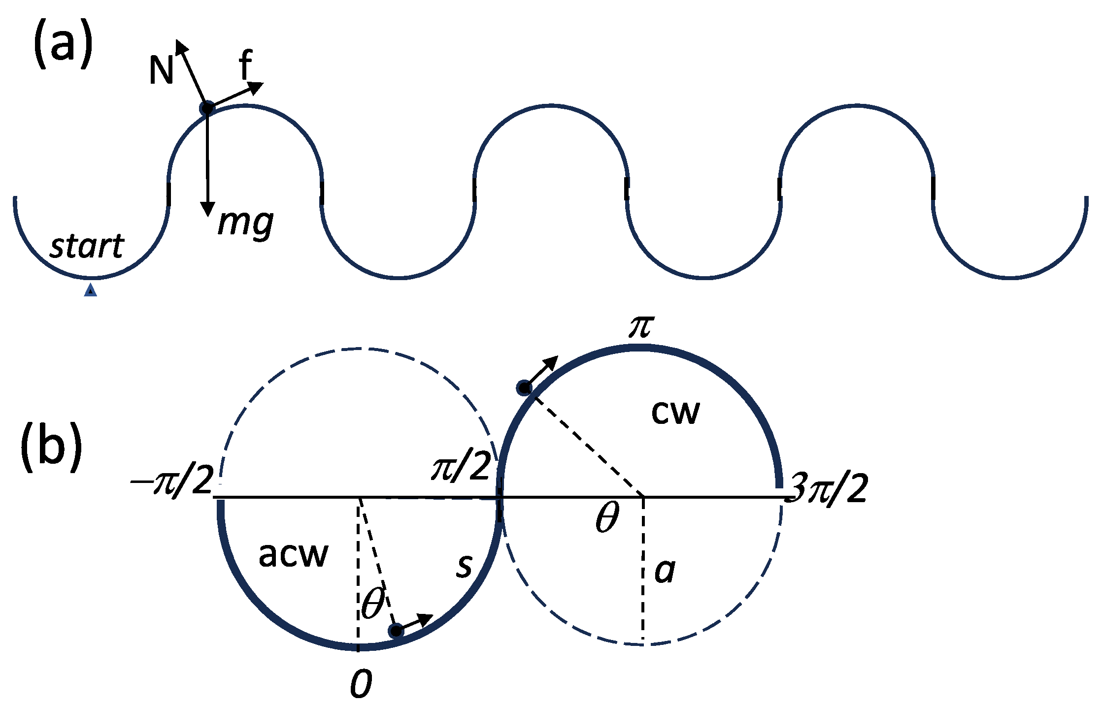
2. Description of a Mechanical Roller Coaster as a Model of a Josephson Junction

To introduce the roller coaster analogy in the simplest way, let us focus straightforwardly on solving a specific exercise, chosen among those involving the basic evolution possibilities of the cart, and on a direct generalization of it. Then, we transpose the solutions, together with their meaning, into the Josephson effect domain.

This analogy traces back to a particular, hardly known, and seldom discussed process occurring in a JJ: we refer to the possibility of ‘dynamical switchings’ of the junction from the zero-voltage state to the resistive state. This analogy seems particularly fitting for this case study, as the authors themselves were able to experience it.

In a ‘dynamical switching’ event, a JJ undergoes unexpected, spontaneous switchings from the zero-voltage state (a condition in which no energy dissipation is present) to the resistive state (a condition in which energy dissipation is present), even in the absence of fluctuations, when solicited by fast signals. In Ref. [15], the phenomenon is introduced and analyzed from the point of view of the theory. Furthermore, it is rightly put in connection with the observed so-called ‘punchthrough’ effect (see [5,7,16] and the references in Ref. [15]). Note that ‘unexpected’ is understood here as ‘for a current lower, or much lower, than the maximum critical current $I_{c0}$ of the junction’ (with values typically in the range of 1 to 10 µA). The maximum critical current of a Josephson junction is the maximum superconducting current observed in that particular junction under ideal laboratory conditions: minimum fluctuations (near zero temperature), quasi-static current variation, perfect magnetic shielding, etc. Given the operation temperature, it is a key quality parameter of the junction. We better illustrate these concepts and their associated nomenclature in Section 6, where we describe the electric behavior of a JJ and define more precisely what one really measures during a ‘junction switching’ event.

Let us also remark that the same exercise we discuss hereafter could have been carried out as well by adopting the classical analogy between a JJ and the winding–oscillating physical pendulum and stress that the emphasis here is on introducing a further educational tool to accompany the existing one.

In the mechanical analogy presented here, a cart is launched from the bottom of one of the valleys for an indefinitely long ride on the roller coaster shown in Figure 1. We suppose, as shown in Figure 1, that there is a suspended track and a small enough cart of mass m that is constrained to the cart. The cart can roll on the track with negligible rolling friction. The trajectory of the cart is a regular sequence of vertical semicircles. The angle $\theta$ determines the position of the track in its clockwise (cw) and anti-clockwise (acw) motion along the roller coaster.

Three forces act on the cart: (a) the weight force $mg$, with g the gravitational acceleration, (b) a constant thrust f pushing the cart, $0\le f\le mg$, and (c) the reaction force of the track. The component of the weight parallel to the track, together with the thrust of the engine, determines the acceleration along the track. In the same way, the component of the weight normal to the track and the track reaction N, both radially directed, provide the transverse acceleration (centripetal acceleration) necessary to drive the cart on the undulated trajectory. The geometry of the roller coaster is simple enough that the equations of motions, one for the parallel and the other for the transverse part of the dynamics, are independent of each other, as occurs in the winding physical pendulum. Thus, for the aims of the consideration given here, one needs to consider only the longitudinal part of the dynamics.

The proposed mechanical model is implementable without significant effort, even though it is only considered as a thought experiment in this paper. Note that an approximately constant thrust parallel to the track can be realized on the macroscopic scale in various ways: rocket engines, water jet engines, or linear electric motors, such as in a certain futuristic roller coaster [17], or in a more modest physics laboratory educational project, by using a small enough cart driven by a fan engine or a propeller.

3. The Equation of Motion of the Mechanical Undulated Suspended Track System

Throughout the study, we assume that the thrust f can be turned on instantaneously to a specific value and maintained at that level for an arbitrary amount of time t. More precisely, we assume $\mathrm{\Delta }t\ll \tau$, with $\mathrm{\Delta }t$ the rise time to the maximum thrust level of the engine and $\tau$ the cart small oscillation characteristic time, i.e., $\tau ={\omega }_0^{-1}$, where ${\omega }_0$ is the cart small oscillation frequency ${\omega }_0={(g/a)}^{1/2}$ (see Appendix B). Additionally, the thrust can be reduced instantaneously, from a higher to a lower value, or even stopped. Therefore, the rise time to the maximum thrust level is fixed to be significantly less than $\tau$, which can be estimated as $\tau$ = 0.5 to 3 s, a time interval ranging from a laboratory model prototype to a hypothetical human-scale amusement park roller coaster with the shape of Figure 1.

The position of the cart on the track is the dynamical variable here. The position is determined, in the curvilinear coordinate system: $s=a\theta$, $-\infty <\theta <+\infty$, by the difference $s-s_0$, where $s_0$ is the point at the bottom of one of the valleys taken as the origin ($s_0=0)$; see Figure 1. The component of the weight force parallel to the track is given by $-mgsin(s/a)$ at any s, as can be verified, and the acceleration of the cart has the form $a(d^2\theta /d{t}^2)$. Under these conditions, the equation of motion, completed by a damping term introduced for further reference ($\mu ds/dt$, with constant coefficient $\mu$), reads as follows:

$$m{\displaystyle \frac{d^{2}s}{d{t}^2}}=-mgsin{\displaystyle \frac{s}{a}}+f-\mu {\displaystyle \frac{ds}{dt}},$$

(1)

which is the equation of a driven-damped pendulum. Note that the sinusoidal form of the gravity force term in Equation (1) is essential for the analogy with a JJ. In the case of the roller coaster, the sinusoidal form arises from the specific shape of the track. To avoid scaling effects and also to obtain a dimensionless quantity capable of representing a phase difference, we express the above equation in a dimensionless form,

$${\displaystyle \frac{d^{2}s}{d{t}^2}}=-sins+\overline{f}-\beta {\displaystyle \frac{ds}{dt}},$$

(2)

which we use in what follows below and where now the lengths are in units of a, time is in units of $\tau$, $\overline{f}=f/mg$, and $\beta =\mu /(m$${\omega }_0$) is a dimensionless damping coefficient (represents the ratio between the small oscillation period and an oscillation damping time $m/\mu$). The velocity is in units of ${\left(ga\right)}^{1/2}$, the acceleration is in units of g, and the energy is in units of $mga$.

Finally, to remind is that the conservative force terms on the right-hand side of Equation (2) can be derived from the potential $U\left(s\right)=1-coss-\overline{f}s$ (an arbitrary constant has been set to 1 such that $U\left(0\right)=0$). This allows us to analyze the motion of the cart in real space, as well as the dynamics of the junction, in terms of a hypothetical particle of the same mass m, falling in the so-called ‘washboard’ or ‘tilted washboard’ potential; a term commonly used in the context of superconductivity [7,8,18]. However, in this paper, we intentionally base the analysis right on the equation of motion in the form of Equation (2), omitting, as much as possible, reference to the washboard potential.

4. An Exercise: Dynamical Condition for the Roller Coaster Ride

Now, let us pose the following question: neglecting damping, and in the conditions described in Section 3 for the engine operation, what is the minimum thrust, ${\overline{f}}_c$, needed to launch the cart in an indefinite duration ride (a ‘running state’), assuming that the cart starts at rest (removable wheel chocks can be used for this aim) from the bottom of a valley (i.e., ${s\left(t\right)|}_{t=0}=0$ and ${ds\left(t\right)/dt|}_{t=0}=0$)?

4.1. The Statics of the Cart

Equation (2) admits two stationary solutions corresponding to two positions on the track, which depend on $\overline{f}$, where $0\le \overline{f}\le 1$, given by $s_1={sin}^{-1}\overline{f}$, and $s_2=\pi -{sin}^{-1}\overline{f}$. At these two points between 0 and $\pi$, which are symmetrically located with respect to $\pi /2$, the vehicle, placed there, remains still with its engine running because the engine thrust well balances the force of gravity. However, while the equilibrium in $s_1$ (located in the interval $[0,\pi /2]$) is stable (except possibly for innocuous small oscillations (see Appendix B), which is not discussed here), that in $s_2$ (a point located in the interval in $[\pi /2,\pi ]$) is critical or unstable (a straightforward perturbation analysis of Equation (2) confirms this circumstance). Practically, if the cart is placed at the instability point $s_2$, with a positive velocity, even though quite small, the cart eventually moves away from $s_2$ and crosses over the top of the hill. As we show in Section 4.2 and Section 4.3 below, this scenario is particularly relevant when the cart starts at rest from the bottom of the track, allowing us to answer the question posed earlier (see Section 4.3).

4.2. The Dynamics of the Cart: Integral of Motion

After multiplying Equation (2) by $\dot{s}$ ($\dot{s}$ denoting $ds/dt$) and integrating in time, one finds the integral of motion:

$${\displaystyle \frac{1}{2}}{\dot{s}}^2-coss-\overline{f}s=\mathrm{const}.$$

(3)

The initial conditions (${s\left(t\right)|}_{t=0}=0$ and ${ds\left(t\right)/dt|}_{t=0}=0$) fix the constant (and the integral of motion) to $-1$ in the exercise under consideration. Equation (3) is the kinetic energy theorem applied to the cart driven along the track: in the absence of dissipation, the overall work done by the applied forces, in going from 0 to s, is equal to the variation in kinetic energy of the body (the material point):

$${\displaystyle \frac{1}{2}}{\dot{s}}^2-0={\int }_0^s(-sinz+\overline{f})dz=coss+\overline{f}s-1.$$

(4)

Incidentally, we note that the integral of motion, represented by Equation (3), corresponds to the conserved total energy. Actually, if one rewrites Equation (4) as $(1/2){\dot{s}}^2+1-coss-\overline{f}s=0$, the latter takes the form of kinetic energy plus potential energy, namely: $(1/2){\dot{s}}^2+U\left(s\right)=0$. We identify the tilted washboard potential as $U\left(s\right)=1-coss-\overline{f}s$. The arbitrary choice $U\left(0\right)=0$ sets the total energy to 0.

Equation (4) gives the velocity as a function of the position in the following form:

$$\dot{s}=\pm \sqrt{2(coss-1+\overline{f}s)}.$$

(5)

From Equation (5), by setting the velocity to zero, i.e., requiring $coss+\overline{f}s-1=0$, one obtains the locus of the points in the (s–$\overline{f}$)-plane, where the velocity of the cart is zero (in addition to the starting point in the origin) as follows:

$$\overline{f}={\displaystyle \frac{1-coss}{s}}.$$

(6)

The relationship (6) is represented graphically in Figure 2a, along with three representative line drawn at the constant thrust values $\overline{f}=0.6,0.7246$, and $0.9$. In Figure 2b, the orbits corresponding to those fixed values of the thrust on the cart were calculated using Equation (5) to give, together with Figure 2a, a qualitative classification of the paths in the phase space, as done in Section 4.3.

4.3. Determining the Value of the Minimum Thrust to Launch the Cart

To obtain information about the minimum thrust, it is necessary to analyze the behaviors depicted in Figure 2 under various thrust conditions. In Figure 2a, the horizontal lines representing constant thrusts can either intersect or not the curve predicted by Equation (6). Let us consider three following cases.

(a)

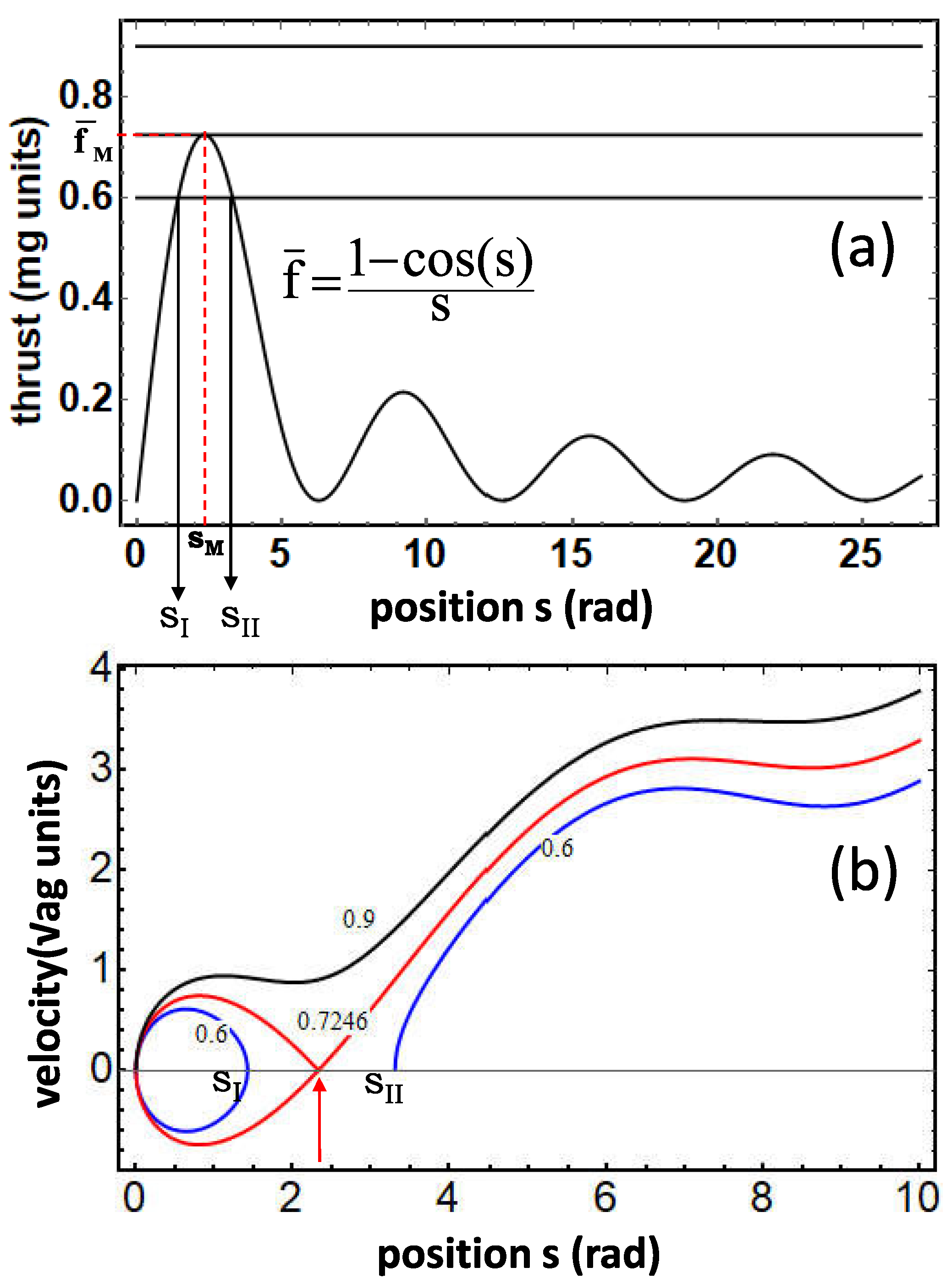
$\overline{f}=0.9$, there can be no an intersection. The thrust exceeds the highest peak of the curve, that is the velocity never reaches zero along the trajectory. In this case, an open orbit is realized. The cart can well start running from the initial position $s=0$ (see Figure 2b, the black curve with $\overline{f}=0.9$).

(b)

$\overline{f}={\overline{f}}_M$, the height of the first peak of the curve in Figure 1a. Now, this specific thrust is exactly the minimum thrust ${\overline{f}}_c$ that is seeking, i.e., the solution to the exercise (as demonstrated in detail in Appendix C). By identifying ${\overline{f}}_c$ with ${\overline{f}}_M$, the value of ${\overline{f}}_M$ can be determined as follows. We solve the equation

$$ssins-1+coss=0$$

(7)

numerically in $(0,\pi ]$ to find $s_M$, the position reached by the cart under the thrust ${\overline{f}}_M$, and calculate ${\overline{f}}_c$ as ${\overline{f}}_c={\overline{f}}_M=sin{s}_M$ (see Appendix C). One finds $s_M=2.33112$ for the position and ${\overline{f}}_c=0.72461$ for the thrust threshold (see in Figure 2b, the red curve, labelled as $\overline{f}=0.7246$).

In brief, ${\overline{f}}_c={\overline{f}}_M$ is the thrust taking the cart from $s=0$ to the instability point $s_c=\pi -{sin}^{-1}{\overline{f}}_c$, where the cart arrives with zero residual velocity. Thus, ${\overline{f}}_c$ is the thrust threshold to launch the cart from $s=0$. Interestingly, at the top of the track ($s=\pi$), the cart has a velocity $\dot{s}\simeq 0.74$ in units of $\sqrt{ga}$, and the cart cannot cross this point at a lower velocity. After reaching the top of the track (or even somewhat earlier, as can be determined by energetic considerations), the engine could also be safely shut off while the cart continues to move by inertia at a constant average velocity. If the engine remains on, the velocity of the cart, in the present approximation of zero damping, continues increasing indefinitely. However, with moderate damping present, the launched cart reaches a dynamical state similar to the ‘inertial’ state where the average velocity remains constant after a transient period. In this energy balance state, the energy lost by drag is continuously provided by the engine thrust (energy balance state).

(c)

$\overline{f}=0.6$, two intersections occur at the points $s_I=1.42$ and $s_{\mathrm{II}}=3.31$, see Figure 2a. No running state is entered. The phase path is a closed orbit, indicating that the thrust on the cart is too weak. As a result, the cart oscillates back and forth between the origin and the point $s_{\mathrm{I}}$, where its velocity reverses cyclically (see Figure 2b, the closed blue curve).

As far as point $s_{\mathrm{II}}$ is concerned, this point marks a position where an open orbit can start, as Figure 2b shows. At this point, the velocity is zero, but the position is different from zero, making this solution, although possible, extraneous to the exercise. The point here is that the integral of motion, Equation (5), does not correspond uniquely to the initial conditions assumed in the exercise. The cart then describe an orbit (an open orbit in the case considered, see Figure 2b, the open blue curve) characterized by the same integral of motion, that is, $-1$ also when it is set at rest in $s_{\mathrm{II}}=3.31$ (shortly after the top) and pushed with the thrust $\overline{f}=0.6$ (the integral of motion is quickly verified to be $-1$ since $-cos{s}_{\mathrm{II}}-0.6s_{\mathrm{II}}=-1$).

Let us summarize. With a step-like rise time thrust corresponding to about the $72\%$ of its weight, $mg$ ($f_c=0.7246$ mg), the cart, in the absence of damping, starting at rest from the bottom of the valley, has enough energy to climb up to the instability point at $\pi -{sin}^{-1}0.7246=2.33$ rad (about $133;30$). A thrust ${\overline{f}}_c+ϵ$ by a relatively small amount $ϵ$ above ${\overline{f}}_c$ puts the cart in the running state for an indefinite time.

5. Further Considerations About the Launch of the Cart

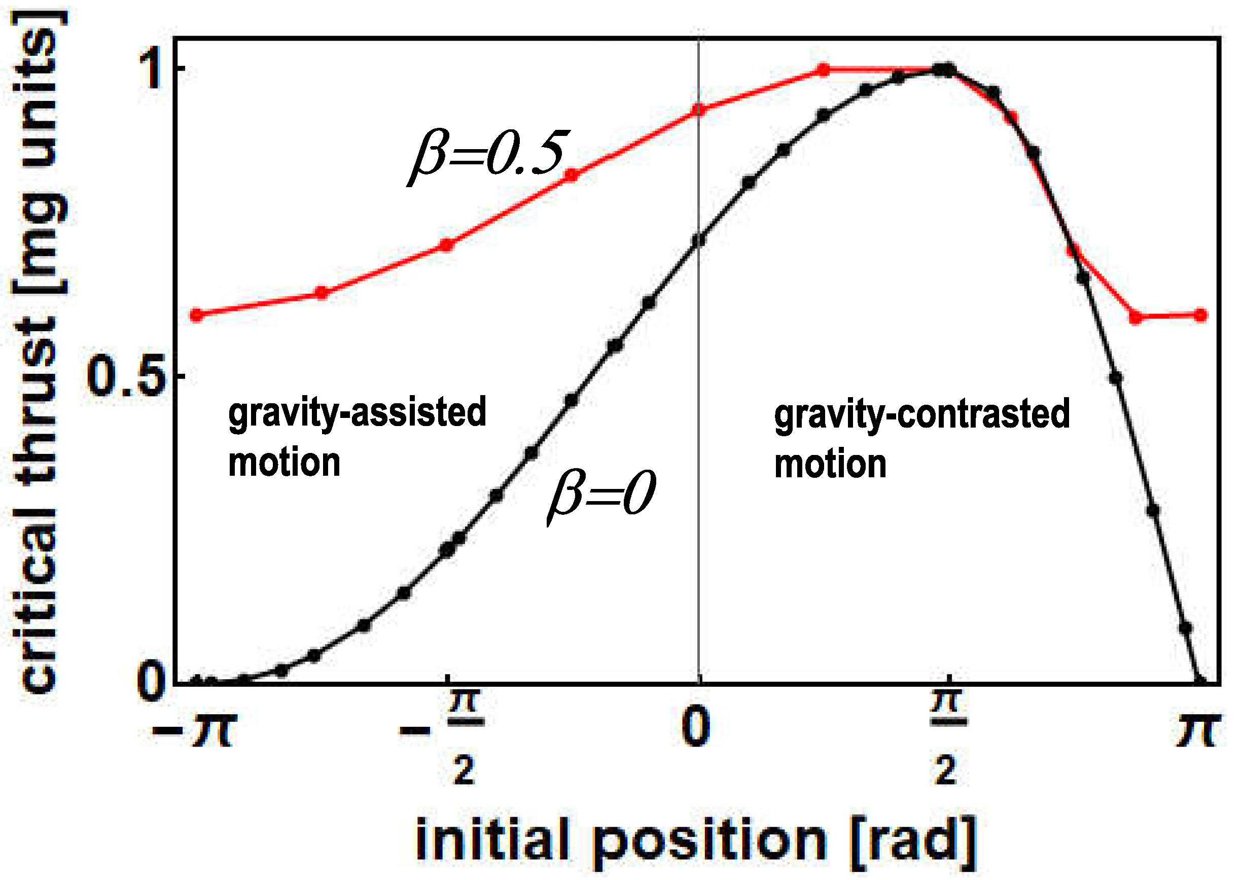
5.1. Minimum Thrust for More General Initial Conditions

The particular threshold found for entering the running state, ${\overline{f}}_c=0.7243$, corresponds to the initial conditions ${s\left(t\right)|}_{t=0}=0$ and ${ds\left(t\right)/dt|}_{t=0}=0$. However, it is possible to achieve lower thresholds than ${\overline{f}}_c=0.7243$ under more general initial conditions, assuming again, as done in Section 4,the idealistic condition of the absence of damping.

Let us suppose, for instance, that the cart oscillates around the zero point in the first valley of the roller coaster, waiting for the ignition (i.e., with $\overline{f}=0$). The maximal elongation is $|s_0|$ ($s_0\in [-\pi ,\pi ]$). And for simplicity, let us assume that at the instant of ignition, the position of the cart is located at the position $s_0$. At this point, the velocity of the cart is also zero, because $s_0$, the maximal elongation point, is an inversion point for the velocity. Then, following the same argumentation as in Section 4.2, Equation (6) is generalized as follows:

$$\overline{f}={\displaystyle \frac{cos{s}_0-coss}{s-s_0}}.$$

(8)

The integral of motion for the new initial conditions is given by ($-cos{s}_0-\overline{f}{s}_0$). Equation (8) represents the locus of the points in the (s–$\overline{f}$)-plane where the velocity of the cart is zero (in addition to the starting point at $s_0$). Again, as in Section 4.3, the critical thrust corresponds to the maximum of the curve defined by Equation (8) in the interval $[0,\pi ]$. The condition $d\overline{f}/d\theta =0$ leads to the equation $coss=cos{s}_0-(s-s_0)sins=0$. Consequently, $\overline{f}=sins$ when used in Equation (8) (this procedure is the same as given in more detail in Appendix C for the case $s_0=0$). Then, assigned $s_0$, we numerically find the root, $s_c$, of $coss=cos{s}_0-(s-s_0)sins$ within the interval $[0,\pi ]$. One then obtains $f_c$ for every $s_0$, either using Equation (8) or just as $\overline{f_c}=sin{s}_c$. This resulting curve is reported in Figure 3 (black line) and represents ${\overline{f}}_c\left(s_0\right)$ in the absence of damping ($\beta =0$).

As can be seen, the choice of the initial positions of the cart can significantly affect the required thrust intensity. For initial positions included between $-\pi$ and $\pi /2$, the minimum thrust needed to reach the instability point $s_2$ and ensure the launching of the cart decreases monotonically from the maximum intensity ($mg$), which occurs at the point $s=\pi /2$ down to zero intensity as $s_0\to -\pi$.

This behavior can be understood by observing that the weight term $-mgsin(s/a)$ changes sign at $s=0$ so that the launch is gravity-assisted ($-mgsin(s/a)$ has the same sign as $\overline{f}$) for $s_0\in [-\pi ,0]$, pointing that the lower thrust value is required, as compared to 0.7246, to reach $s_2$. In contrast, for $s_0\in [0,\pi /2]$, the launch is gravity-contrasted ($-mgsin(s/a)$ has a sign opposite to $\overline{f}$), requiring the value up to 1, compared to $0.7246$, to reach $s_2$. For initial positions beyond $\pi /2$, the minimum thrust required starts decreasing again (reaching 0 for $s_0=\pi$). This is because the motion of the cart remains gravity-contrasted, but the gravity term $-mgsin(s/a)$ gradually disappears.

5.2. Quasi-Static Launch

In contrast with the impulsive thrust mechanism (sudden ignition to a constant thrust level with a consequent dynamical launch of the cart) described in Section 4, one can also imagine an ‘adiabatic’ or quasi-static launch operation. The thrust on the cart is ramped up quite slowly, such that the cart moves (starting at rest from $s_0=0$) slowly enough, i.e., with a velocity and acceleration close to zero. The thrust ramps in time between 0 and 1 so that the mass can adjust its position to reside all the time in the equilibrium point $s_1$ or highly close to it: $s_1\left(t\right)\approx {sin}^{-1}\left(\overline{f}\left(t\right)\right)$.

When $\overline{f}=1$, the position of the cart is $s_1=s_2=s=\pi /2$ and the cart is well vertical, held up by a thrust equal to its weight in an unstable equilibrium on the track. In this condition, it is impossible to increase the thrust, even slightly, without entering the running state of the cart. Certainly, this kind of launch operation necessarily requires a thrust equal to the weight of the cart at some point ($s=\pi /2$).

Finally, it is to be stressed that, more broadly, one can operate between a sudden ignition launch and a quasi-static launch by linearly ramping the thrust on the cart to a specific value $\overline{f}$ (${\overline{f}}_c<\overline{f}<1$) with a ramp duration $\Gamma$ ($0<\Gamma <\infty$). In this case, for each different $\Gamma$ value, a different threshold ${\overline{f}}_c$ can be determined (above $0.7246$) such that a dynamical launch is feasible for values of $\overline{f}$ between the found ${\overline{f}}_c$ and 1 (for instance, using trapezoidal AC (alternative current) supply current, in the case of a JJ). Let us refer to Figure 3 in Ref. [15] for a visual representation of the two different scenarios, with necessary adjustments.

5.3. Considerations About the Damping

In the presence of damping, the potential to start the cart with a thrust less than the weight of the cart—discussed in Section 4—is significantly obscured or may even disappear. Let us notice, at this stage, that in the case of the cart, the velocity-dependent damping term $\mu ·ds/dt$ in Equation (1) needs to be identified, to illustrate more practically this point, with the effect of the air resistance (drag resistance) on the cart. As so, all the achievable steps need to be taken to reduce the rolling friction (rigid wheels–track contact, lubrication of the bearings, etc.).

The disappearance of the potential to realize a ’dynamical launch’ in the presence of damping is illustrated schematically in Figure 3. The red curve has been calculated numerically in the presence of damping, for $\beta =0.5$ ($\beta >1$ is the overdamped regime, recalling that $\beta =\tau /(m/\mu )$), for reference purposes. It is understandable the mitigation of the possibility of using a diminished thrust, as compared with $mg$ for the launch (for instance, starting the launch from zero, one numerically obtains that $f_c$ changes from values of 0.7246 to 0.7746, 0.9346, and 0.9815, for $\beta$ values of 0.1, 0.5, and 0.7, respectively). For $\beta \approx 1$, the thrust requirement is, in practice, 1, for any $s_0$ value.

To stress, however, is that it is always possible to launch the cart, even with exceptionally high damping, by using a thrust not exceeding $mg$ (the minimum thrust needed is always, at most, $mg$). Indeed, suppose that $\beta \to \infty$ (worst hypothesis); then, the equation of motion becomes

$$\beta {\displaystyle \frac{ds}{dt}}=\overline{f}-sins.$$

(9)

The minimum thrust to have the cart riding indefinitely, disregard the initial condition, is ${\overline{f}}_c=1$. Recently, in Ref. [18], the case of overdamped junctions has been studied based on Equation (9), with a special reference to the pendulum as a mechanical analog.

6. Analogous to What? (Equation of Motion for the Phase in a Josephson Junction)

As a next step, in this Section, we revisit the conceptual steps leading to the equation of motion for the phase in a JJ. In the equation derived for the junction, the reader can recognize Equation (1) and can make the due connections. The two main components here are the Josephson equations and a circuital schematization of a real superconducting junction.

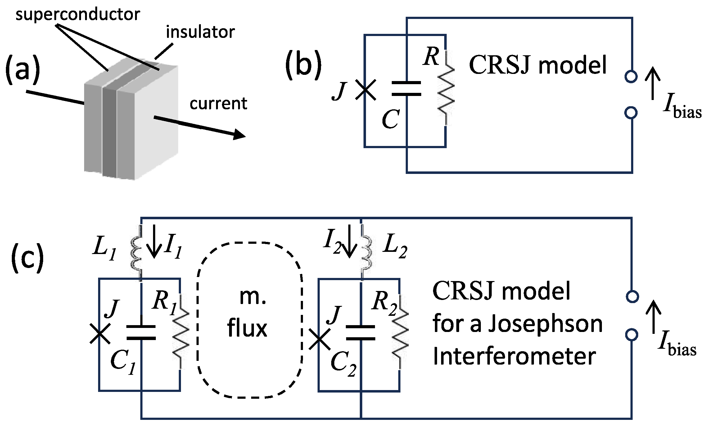
6.1. The Josephson Equations

Brian Josephson first [10,11] suggested that when two superconductors are sufficiently close to each other, for instance, separated over a quite small contact area by a thin (few nanometers) insulating oxide layer, and connected to a current source, a dissipationless current made of coupled electrons (Cooper pairs) can flow by tunneling between the electrodes with no voltage difference. Josephson also predicted successfully [19] that:

(a)

The supercurrent depends on the macroscopic quantum phase difference between the two superconductors $\phi \left(t\right)={\theta }_1-{\theta }_2$. This relationship is described by the equation $I_J\left(t\right)=I_{c0}sin\left(\phi \left(t\right)\right)$ (current–phase relation), where $I_{c0}$ is the maximal critical current, i.e., the highest supercurrent that the junction can support.

(b)

When the bias current $I_{\mathrm{bias}}$ changes over time, as controlled by a current supply, a voltage difference is generated across the junction. The instantaneous value of this voltage is given by $V\left(t\right)=(\hslash /2e)d\phi \left(t\right)/dt$ (voltage–phase relation), with ℏ the reduced Planck’s constant and e the elementary electrical charge. Note that the proportionality factor ($\hslash /2e$), in the above voltage-phase relation, solely involves universal constants, which marks the macroscopic quantum nature of the effect.

6.2. CRSJ Model

Despite the quantum nature of the phase difference, a real junction (sketched in Figure 4a) may be characterized by measurements of current and voltage and treated, for most purposes, as an ordinary electric element governed by classical electromagnetism.

Actually, it can be effectively described as a parallel circuit consisting of three distinct current channels (Figure 4b): a capacitive channel ($I_C=CdV/dt$, where C is the geometric capacitance between the two electrodes), a resistive channel ($I_R=V/R$, where R is the resistance), and a superconducting channel ($I_J=I_{c0}sin\phi$). This often-used schematization (known as resistively and capacitively shunted junctions, or the CRSJ model) allows us to derive, via current balancing, i.e., $I_{\mathrm{bias}}=I_C+I_R+I_J$, and through use of the voltage–phase relation, the following equation for the time evolution of the phase $\phi$, in analogy to Equation (1) for the position of the cart on the track:

$${\displaystyle \frac{\hslash }{2e}}C{\displaystyle \frac{d^2\phi }{d{t}^2}}=-I_{c0}sin\phi +I_{\mathrm{bias}}-{\displaystyle \frac{\hslash }{2e}}{\displaystyle \frac{1}{R}}{\displaystyle \frac{d\phi }{dt}}.$$

(10)

Rather unexpectedly, a lower resistance results in higher dissipation, as the dissipative term is proportional to $1/R$. This happens because the resistance R is placed in parallel to the superconducting branch. The lower the resistance, the higher the normal current generated by normal electrons, leading to higher dissipation. To obtain an overdamped junction (useful in many applications), one has to use lower R values.

Equation (10) describes two possible regimes: below $I_{c0}$, Equation (10) describes a regime when the average value of $d\phi /dt$ is zero (the zero-voltage state). In general, the phase stabilizes around the constant value $\overline{\phi }={sin}^{-1}(I_{\mathrm{bias}}/I_{c0})$, the static stable solution of Equation (10). In contrast, when the bias current $I_{\mathrm{bias}}$ exceeds $I_{c0}$, Equation (10) describes a dissipative regime (finite voltage state). In this regime, a current of normal electrons (quasiparticle) adds to that of Cooper pairs—actually the two currents coexist—and a finite voltage (the average value of the oscillating term, $d\phi /dt$), together with a finite resistance appears across the junction. Here, the averages are taken as $\langle d\phi /dt\rangle ={lim}_{\mathcal{T}\to \infty }(1/\mathcal{T}){\int }_0^{\mathcal{T}}\left(d\phi /dt\right)dt$, and the implicit assumption is made that the bias current, $I_{\mathrm{bias}}$, changes in a quasi-static manner, i.e, on a time scale considerably larger than ${\tau }_J={\omega }_J^{-1}$, the characteristic time scale of the Josephson plasma oscillation, so that the threshold separating the two regimes is $I_{c0}$ (not a fraction of $I_{c0}$ as occurs in dynamical switching). Here, in the definition of ${\tau }_J$, ${\omega }_J$ is the Josephson plasma frequency, i. e., ${\omega }_J={(2e{I}_{c0}/\hslash C)}^{1/2}$, an analog to the inverse cart small oscillation frequency ${\omega }_0$. The crossing of the threshold $I_{c0}$, with the related onset of a voltage between the two junction electrodes, is the ‘switching’ of the junction.

The quasi-static operation described for the cart in Section 5.2 is close to the experimental protocol typically used to characterize a junction in terms of its maximum Josephson current. However, unlike the cart case, one has no control over the initial conditions concerning the junction phase difference. The current is gradually increased, starting from zero, at quite a slow sweep rate until a switching is observed from the zero-voltage state to a finite-voltage state at a specific current $I_c$. It is reasonable to assume that this observed critical current value $I_c$ is the best approximation of the ‘ideal’ maximum critical current $I_{c0}$ at the operation temperature of the junction. On the other hand, since the plasma frequency for a Josephson junction is extremely high (in the terahertz range), it becomes challenging to increase the current on a timescale shorter than the plasma period, except using special equipment under specific laboratory conditions. Another significance affecting the current at which a junction switches to the finite-voltage state is noise, particularly thermal fluctuations. Even close to absolute zero temperature, quantum fluctuations remain, affecting the performance of the junction. The ideal critical current $I_{c0}$ may be defined by the absence of fluctuations and the quasi-static operation of current control.

Equation (10) is rewritten in dimensionless form as follows:

$${\displaystyle \frac{d^2\phi }{d{t}^2}}=-sin\left(\phi \right)+\alpha -{\beta }_J{\displaystyle \frac{d\phi }{dt}},$$

(11)

where time is in units of ${\tau }_J$, $\alpha =I_{\mathrm{bias}}/I_{c0}$, and ${\beta }_J$$={\left({\omega }_{J}RC\right)}^{-1}$ is a dimensionless damping coefficient (Johnson parameter [5]). In these units, the voltage is in units of ${(\hslash I_{c0}/2eC)}^{1/2}$, and the energy is in units of $\hslash I_{c0}/2e$. In

Table 1. Correspondence between physical quantities in the JJ CRSJ model and in the cart mechanical analog. See text for details.

Electric Analog (CRSJ Model)	Mechanical Analog (Cart)
junction capacitance coefficient $\hslash C/2e$	mass of the cart m
damping parameter ${\displaystyle \frac{\hslash }{2e}}(1/R)$	damping parameter $\mu$
phase difference $\phi$	dimensionless position of the cart $s/a$.
bias current $I_{\mathrm{bias}}$	thrust on the cart f
maximal Josephson critical current $I_{c0}$	weight of the cart $mg$
instantaneous voltage ${\displaystyle \frac{\hslash }{2e}}d\phi /dt$	velocity $ds/dt$
Josephson plasma frequency ${\omega }_J={(2e{I}_{c0}/\hslash C)}^{1/2}$	cart small oscillation frequency ${\omega }_0={(g/a)}^{1/2}$
Josephson current $I_{c0}sin\phi$	weight parallel component $mgsin\left(s/a\right)$

, the corresponding elements of the CRSJ model (sometimes referred to as the ‘electric analog’ of a Josephson junction) and mechanical analog introduced in this paper are reported.

6.3. Analogy Highlights

Let us summarize the main points characterizing the analogy between the dynamics of a Josephson junction and those of a cart on the roller coaster.

(a)

The bias current $I_{\mathrm{bias}}$ in the junction corresponds to the thrust $\overline{f}$ on the cart. The weight $mg$ of the cart corresponds to the critical current $I_{c0}$ of the junction.

(b)

Two regimes are individuated in the dynamics of the cart: one regime when the cart remains trapped in a valley, and another regime when the cart rides on the track, according to whether the thrust f acting upon it reaches the value $mg$. In the same way, two regimes exist in the junction phase dynamics, a zero-voltage state and a finite voltage state according to whether $I_{\mathrm{bias}}$ reaches or overcomes $I_{c0}$.

(c)

The ‘launch attempts’ (failed attempts) experienced by the cart at the bottom of a valley of the roller coaster, under the action of an insufficient thrust, lesser than the requested weight $mg$ of the cart, correspond to the zero-voltage regime of the junction. In this state, the phase difference undergoes the same kind of bound oscillations as the position of the cart experiments, and the junction is unable to develop a finite voltage state.

(d)

The riding of the cart on the roller coaster corresponds to the finite voltage state of the junction. In this analogy, both dynamical variables $s\left(t\right)$, the position of the cart (in units of a) along the track, and $\phi \left(t\right)$, the phase difference between the two superconducting electrodes of the junction, increase over time, without limits. Both the variables are characterized by a finite average rate of growth: the average velocity of the cart in the mechanical analog corresponds to the average voltage across the two electrodes in the junction.

(e)

Experimentally, it can be observed under measurement conditions of fast current polarization, that a JJ can switch to the finite voltage state even when $I_{\mathrm{bias}}$ reaches values lower than the critical Josephson current $I_{c0}$. Using the present didactic approach we have shown how the mechanical equivalent shows positively this peculiar effect.

It should be stressed at this point that, although analogous, the two systems remain significantly different. Apart from the characteristic times, differing for a factor between ${10}^{10}$ and ${10}^{15}$, there is the essential aspect related to the thermal fluctuations. Thermal noise has a critical impact on the performances of a JJ and is actually the major factor with detrimental effects on the critical current. The Josephson coupling energy $\hslash I_{c0}/2e$ is typically of $1.2\times {10}^{-2}$ eV ($I_{c0}\approx 1$ µA and the thermal noise fluctuations’ typical value is $k_B$$T_K$ $\approx 8.6\times {10}^{-3}$ eV (corresponding to a typical ’noise temperature’ $T_K\approx$ 100 K, with standard noise screening conditions), where $k_B$ is the Boltzmann constant. That is, the phase difference can well enter the domain of a random variable subject to thermal fluctuations, even close to absolute zero.

6.4. Dynamical Switching and ‘Punchthrough’ Effect

What remains of the exercise carried out for the roller coaster in the domain of a JJ? The answer is: the effect described in Section 4 (the ’dynamical launch’ of the cart) corresponds to the possibility of observing ‘a dynamical switching’ event in an underdamped JJ. The underdamped condition is matched in high capacitance–high resistance junctions, in agreement with the definition of ${\beta }_J$.

It is worth to describe more closer what one really observes during a ‘dynamical switching’ event: initially, there is a junction in the zero-voltage state (see Section 6); then, the current i is increased from an initial value $i_1$ (can be zero) to a bigger value $i_2$, lower than the critical current $I_{c0}$ (but higher than a threshold $i_c>i_1$), in a quite short time $\mathrm{\Delta }t$, considerably shorter than the characteristic time ${\tau }_J$ (typically of ${10}^{-10}$–${10}^{-9}$ s). Under this condition of fast increment, the new value of current is unstable for the zero-voltage state. That is, after the current has reached the value $i_2$, the junction switches stably to the finite voltage state (the time it takes depends sensitively on $i_2$, as estimated in Appendix D). Had the current $i_2$ been reached gradually or more gradually in comparison with ${\tau }_J$ ($\mathrm{\Delta }t\gg {\tau }_J$), no such switch to be observed at the current value $i_2$. The junction then just remains on the superconducting current branch, with that new value of the current and zero voltage across the electrodes. This, in practice, constitutes an effective reduction of the junction critical current and is ultimately an issue to be taken into account for fast enough signals.

The mechanism is completely analogous to the critical dynamical launch of the cart: the current value is raised instantaneously to the critical value of $0.7246I_{c0}$. This is sufficient to make the phase reach the unstable value ($\pi -{sin}^{-1}0.7246$), from which a finite voltage regime starts ($\langle \dot{\phi }\rangle \ne 0$, i.e., $\langle V\rangle \ne 0$).

In certain applications that use JJs in the latching mode, such as logic circuits that need to be rapidly reset to the zero-voltage state from the finite-voltage state, this effect assumes a special form, known as ‘punchthrough’, which can be particularly detrimental. In an emphasized image, the junction ‘refuses’ to remain on the dissipationless Josephson current branch when needed, as first studied in Ref. [16].

Let us stress that this occurs because the current in the junction is rapidly swept. We notice in passing that high-sweep-rate signals (’pulsed’ excitation) have been used in the recent past in connection with the CRSJ model to make to emerge interesting and unusual nonlinear behaviours whose features mimic macroscopic quantum effects in JJs (see Ref. [21] and the references therein).

Finally, it is useful to remark that while thermal fluctuations cannot be completely eliminated, as well as the fundamentally present quantum noise, dynamical switchings can, in principle, be controlled. This can be accomplished in cases where it is acceptable to operate with an overdamped junction. By shunting the junction with an appropriate resistance, the damping term in Equation (10) can be made dominant. Actually as seen in Section 5.3, friction prevents using a thrust lesser than $mg$ for the launching of the cart, the red curve in Figure 3; in the same way, damping mitigates or also impedes the possibility of premature switchings in JJs.

7. Two-Cart Train Roller Coaster: A Josephson Interferometer

How far can the roller coaster analogy with a Josephson junction be carried on? In this Section, we indicate the most natural extension of this analogy: the presence of more than a single JJ. Specifically, we consider superconducting circuits containing N coupled point-like junctions in parallel, which is a discrete version of a so-called ‘long Josephson junction’ [5,6,7,8], a junction where the size causes the phase difference to depend on both position and time.

The mechanical analog for an array of this kind is represented by a roller coaster train made by a series of N elastically coupled carts whose positions $s_1,s_2,\dots ,s_N$ represent the values of the N phase differences ${\phi }_1,{\phi }_2,\dots ,{\phi }_N$. This identification is reminiscent of the known extension of the pendulum analogy for a single junction to a parallel array of JJs, represented by a chain of coupled winding pendulums [22] (see also Ref. [5], p. 265). In such a mechanical device, as well as in a train of several carts riding the roller coaster, true waves can propagate (along the train); likewise, phase waves (linear and nonlinear) can propagate in a long enough JJ.

We now examine a fundamental case of possible extensions to arrays of junctions: that of a circuit made by two junctions connected in parallel, commonly referred to as a ‘Josephson interferometer’ (or dc SQUID, ‘direct current Superconducting Quantum Interference Device’) (Figure 4c). In the circuit shown in Figure 4c, a superconducting current splits between the two channels $I_1=I_{c0}sin{\phi }_1$ and $I_2=I_{c0}sin{\phi }_2$ with two phase differences ${\phi }_1$ and ${\phi }_2$, respectively. These currents can flow without generating voltage across the two resistances until a maximum current is reached. Beyond this threshold, the circuit starts oscillating.

The maximum current (the maximum Josephson current of the SQUID) is a highly sensitive function of the magnetic field normally applied to the plane of the circuit. This serves as a basis for advanced magnetometers. In this case, the mechanical analogy consists of a roller coaster train made by two coupled in-line carts riding the roller coaster track of Figure 1 (see Figure 5).

Let us consider two carts, labeled 1 and 2, which have vanishing dimensions and the same mass m. Their positions on the track are designated by $s_1$ and $s_2$, respectively, so that the train is ($s_2-s_1$)-long. The carts are connected by an articulated rod (with inserts of elastic material) of negligible weight compared to that of each cart (Figure 5). Let us assume that the rod rolls on and is constrained to the track like the carts themselves; as noted, it is elastically deformable to a certain degree (thanks to the inserts) and is similar to a stiff spring with an elastic constant k.

We also assume that a thrust F acts on cart 2, driving the entire train (in the circuit of Figure 4c, this corresponds to the asymmetric situation in which one of the two self-inductance coefficients $L_1$, $L_2$, has a value much smaller than the other). Under these conditions, the length of the train ($s_2-s_1$) depends on the mechanical tension T to which the rod is subject. The dynamics of the two coupled carts must include, besides T and F, the effect of the weight components $P_1=-mgsin{s}_1$ and $P_2=-mgsin{s}_2$ on carts 1 and 2, respectively (see Figure 5a for a sketch of the forces). Thus it is determined by the following equations (the friction is neglected as in the consideration in Section 2, Section 3, Section 4 and Section 5 above):

$$\begin{array}{ccc}& & m{\displaystyle \frac{d^2{s}_2}{d{t}^2}}=F-T-mgsin{s}_2,\hfill \end{array}$$

(12)

$$\begin{array}{ccc}& & m{\displaystyle \frac{d^2{s}_1}{d{t}^2}}=T-mgsin{s}_1,\hfill \end{array}$$

(13)

where $s_1$ and $s_2$ also satisfy the following:

$$s_2-s_1=H+kT$$

(14)

Here, H is the length of the unsolicited ($T=0$) train, and $kT$ is the change in length of the train, assumed to be proportional to T through k.

In the dimensionless time and length, the following apply:

$$\begin{array}{ccc}\hfill & & {\displaystyle \frac{d^2{s}_2}{d{t}^2}}=\overline{F}-\overline{T}-sin{s}_2,\hfill \end{array}$$

(15)

$$\begin{array}{ccc}\hfill & & {\displaystyle \frac{d^2{s}_1}{d{t}^2}}=\overline{T}-sin{s}_1,\hfill \end{array}$$

(16)

$$\begin{array}{ccc}\hfill & & s_2-s_1=H+\kappa \overline{T},\hfill \end{array}$$

(17)

where $\overline{F}=F/mg$, $\overline{T}=T/mg$, and $\kappa =kmg/a$ is the reduced elastic constant.

7.1. On the Statics and Dynamics of a Two-Cart Train of an Assigned Length ($\kappa =0$)

Let us write the equation of motion for the relative position $s_d=(s_2-s_1)$ and the center of mass $s_s=(s_1+s_2)/2$. To this end, we add and subtract Equations (15) and (16) to write the following:

$$\begin{array}{ccc}\hfill & & 2{\displaystyle \frac{d^2{s}_s}{d{t}^2}}=\overline{F}-2sin{s}_{s}cos{\displaystyle \frac{s_d}{2}},\hfill \end{array}$$

(18)

$$\begin{array}{ccc}\hfill & & {\displaystyle \frac{d^2{s}_d}{d{t}^2}}=\overline{F}-2\overline{T}-2cos{s}_{s}sin{\displaystyle \frac{s_d}{2}}.\hfill \end{array}$$

(19)

In a simplified case of $\kappa =0$ (rigid connection between the two carts), one just has $s_d=s_2-s_1=H=\mathrm{const}.$, and one obtains the following from Equation (18) (requiring $d^2{s}_s/d{t}^2=0$):

(a)

The equilibrium points for the center of mass $s_s$, similar to the stationary points $s_1$ and $s_2$ of the single cart,

$$\begin{array}{c}\hfill S_1={sin}^{-1}{\displaystyle \frac{\overline{F}}{2cos\frac{H}{2}}},\\ \hfill S_2=\pi -{sin}^{-1}{\displaystyle \frac{\overline{F}}{2cos\frac{H}{2}}}.\end{array}$$

(b)

The limits of the static equilibrium for the two rigidly coupled cart trains. That is:

$$F_c=\underset{s_s\in [0,2\pi ]}{max}\left[2sin{s}_{s}cos{\displaystyle \frac{H}{2}}\right]=2\left|cos{\displaystyle \frac{H}{2}}\right|.$$

(20)

Assigned H, there is a corresponding thrust, $\overline{F}$, and a corresponding position of the center of mass ($S_1$) that allows the train to remain stationary at $S_1$. However, when the required thrust for the assigned value of H exceeds a threshold $F_c$, the train can no longer maintain static equilibrium and begins to move. The threshold curve $F_c$ versus H is a periodic function of H and is fully defined by Equation (20).

In particular, a train of length $H=\pi$ (or $3\pi$, or $5\pi$, …) does not require any force $\overline{F}$ to be kept still on the track as soon as in this case, Equation (20) gives ${\overline{F}}_c=0$. Regardless of its position, the train remains there in a static indifferent equilibrium under the influence of gravity and tension T. In other words, an infinitesimal thrust $\overline{F}\simeq 0$ is needed to make the train of length $\pi$ move against gravity along the roller coaster (surely, the friction remains to be overcome, just as a train on a well flat track). Equation (19), with $H=\pi$ and $\overline{F}=0$, provides the value of the tension for any position of the center of mass of the train, $s_s$, as $T=-cos{s}_s$.

The resulting Equation (20) is known in the Josephson effect domain. As well, Equation (20) is analogous to the form of the two-slit interference pattern of optics. The latter describes the diffraction pattern displayed by the critical current in a Josephson interferometer in response to an applied magnetic flux and is the basis of a dc SQUID magnetometer. In the analogy, the role of the flux is played by the length H of the two-cart train.

(c)

The critical thrust to launch the train formed by two carts (dynamical switching of a SQUID). We follow here the same consideration as that in Section 4.2. Equation (18), with the initial conditions ($s_s{\left(t\right)|}_{t=0}=0$ and $d{s}_s{\left(t\right)/dt|}_{t=0}=0$), admits the integral of motion:

$${\dot{s_s}}^2-2cos{s}_{s}cos{\displaystyle \frac{H}{2}}-F{s}_s=-2cos{\displaystyle \frac{H}{2}}=\mathrm{const}.$$

(21)

Thus, the velocity as a function of the position on the track can be obtained as follows:

$${\displaystyle \frac{d{s}_s}{dt}}=\sqrt{\left(\overline{F}{s}_s+2cos{\displaystyle \frac{H}{2}}(cos{s}_s-1)\right)}.$$

(22)

From the condition that Equation (22) equals zero, one finds the generalization of Equation (6):

$$\overline{F}={\displaystyle \frac{\left(1-cos{s}_s\right)2cos\frac{H}{2}}{s_s}}.$$

(23)

The thrust is maximum at $s_s=2.33112$, where it takes the following value:

$$\overline{F_c}=2·0.7246\left|cos{\displaystyle \frac{H}{2}}\right|.$$

(24)

7.2. Mechanical Analog of the Self-Flux: Elastically Coupled Carts ($\kappa \ne 0$)

Most interestingly, as noted in Section 7.1 just above, the length of the train H (or the length of the rod that is the same) plays the same role here that the externally applied magnetic flux plays in a Josephson interferometer.

The analogy extends further: one can distinguish between this component of the flux, identified with the length of the unstrained train ($\kappa =0$), and the self-induced flux component, i.e., the part of the flux generated in the interferometer loop by the circulating currents themselves (then, $\kappa$ plays the same role as the self-inductance of the loop containing the flux in Figure 4c). This latter is to be identified with the changes in the length of the train when it is solicited and when it is not solicited. Indeed, the train stretches or shortens to a certain degree under its own weight ($\kappa \ne 0$). When it stands in a valley, it shortens due to the compressing gravity effect. On the contrary, hanging in equilibrium on a top, it is stretched by the pulling gravity effect.

Therefore, one can talk about a ‘total length’ of the train: the one corresponding to its length in the absence of stresses (at rest on a flat track), plus the contribution due to self-deformation in the presence of stresses. Likewise, in a Josephson interferometer, one can talk about ‘total flux’ and ‘external flux’, whose difference is the self-induced flux.

Let us analyze the case $\kappa \ne 0$ more closely. In particular, one can evaluate the equivalent of the equilibrium curve ${\overline{F}}_c\left(H\right)$ (Equation (20)) for the case of two elastically coupled carts on the roller coaster (the results are graphically illustrated in Figure 6).

To obtain these results, let us address to Equations (15)–(17). The static part reduces to the following:

$$\begin{array}{ccc}\hfill & & \overline{F}=sin{s}_1+sin{s}_2,\hfill \end{array}$$

(25)

$$\begin{array}{ccc}\hfill & & \overline{T}={\displaystyle \frac{\overline{F}}{2}}+{\displaystyle \frac{sin{s}_1-sin{s}_2}{2}},\hfill \end{array}$$

(26)

$$\begin{array}{ccc}\hfill & & s_2-s_1=H+\kappa \overline{T}.\hfill \end{array}$$

(27)

One can eliminate $s_2$ and obtain the following expression for $\overline{F}$:

$$\overline{F}=sin{s}_1+sin\left(s_1+H+\kappa sin{s}_1\right),$$

(28)

which can be (numerically) maximized with respect to $s_1$ (choose $\kappa$, then for each H, calculate $\overline{F}$ as $s_1$ varies in the interval $[0,\pi ]$, take the maximum $\overline{F}$, build ${\overline{F}}_c\left(H\right)$) (Figure 6, curve a).

In the same way, we consider the more symmetric case of a train pulled and pushed at the same time; that is, it can be assumed that both carts, 1 and 2, are equipped with an engine producing half of the thrust $\overline{F}$ (see Figure 5d; in Figure 4c, this corresponds to having $L_1\eqsim L_2$). It can be shown that Equation (28) transforms into the following:

$$\overline{F}=sin{s}_1+sin\left[s_1+H+\kappa \left(sin{s}_1-{\displaystyle \frac{\overline{F}}{2}}\right)\right].$$

(29)

Equation (29), differently from Equation (28), is an implicit equation for $\overline{F}$. The procedure to build ${\overline{F}}_c\left(H\right)$, however, is the same, but an additional step is needed to solve the above implicit Equation (29) numerically (Figure 6, curves b and c).

The curves shown in Figure 6 were calculated using Equations (28) and (29) by using MATHEMATICA (version $11.2.0.0$) programming. These curves are also known in the physics of superconducting Josephson interferometers [20,23]. For a general analytical approach to the response of a Josephson interferometer, see Ref. [24].

Along the line obtained in this Section, one can consider the case of a multi-cart elastic train of arbitrary length and number of carts (unpractical for a mechanical prototype compared with a chain of pendula, we admit). This step brings us to the territory of the Frenkel–Kontorova model [25,26] (and, in particular, the sine-Gordon equation [27]). Indeed, the simplest realization of the Frenkel–Kontorova model is a chain of N particles interacting via harmonic springs with elastic coupling and subjected to the action of an external periodic potential; in the case considered here, the tilt washboard potential.

8. Conclusions

In the work presented, we have illustrated a mechanical analogy for the dynamics of a JJ; specifically, an alternative way to realize a tilted washboard potential for a material point. A cart on a vertically winding roller coaster driven by a constant force possesses the same dynamics of a JJ. Both systems are governed by the same equation of motion. To explain the details of the analogy and its use as an educational tool, we have taken a cue from a particular possible evolution of the cart: a departure of the cart for a long ride from a valley of the track when pushed by a step-like thrust, which we refer to as ‘the launch of the cart’. In a JJ, this mechanical process has its equivalent in a premature switching (dynamical switching) of the junction to the finite voltage state, not related to the presence of noise. Furthermore, we have extended the analogy to the case of two coupled carts (a train) riding over the roller coaster, demonstrating that this extension is a mechanical analog of a Josephson interferometer.

References

1. Citro, R.; Guarcello, C.; Pagano, S. Josephson junctions, superconducting circuits, and qubit for quantum technologies. In New Trends and Platforms for Quantum Technologies; Aguado, R., Citro, R., Lewenstein, M., Stern, M., Eds.; Springer: Berlin/Heidelberg, Germany, 2024; pp. 1–59. [Google Scholar] [CrossRef]
2. Dejpasand, M.T.; Ghamsari, M.S. Research trends in quantum computers by focusing on qubits as their building blocks. Quant. Rep. 2023, 5, 597–608. [Google Scholar] [CrossRef]
3. Kjaergaard, M.; Schwartz, M.E.; Braumüller, J.; Krantz, P.; Wang, J.I.-J.; Gustavsson, S.; Oliver, W.D. Superconducting qubits: Current state of play. Annu. Rev. Condens. Matter Phys. 2020, 11, 369–395. [Google Scholar] [CrossRef]
4. Martinis, J.M. Course 13—Superconducting qubits and the physics of Josephson junctions. In Les Houches 2003: Quantum Entanglement and Information Processing; Estève, D., Raimond, J.-M., Dalibard, J., Eds.; Elsevier B.V.: Amsterdam, The Netherlands, 2004; pp. 487–489, 491–520. [Google Scholar] [CrossRef]
5. Barone, A.; Paternò, G. Physics and Applications of the Josephson Effect; John Wiley & Sons, Inc.: New York, NY, USA, 1982; Chapter 6. [Google Scholar] [CrossRef]
6. Mangin, P.; Kahn, R. Superconductivity. An Introduction; Springer International Publishing AG: Cham, Switzerland, 2017; Chapter 10. [Google Scholar] [CrossRef]
7. Likharev, K.K. Dynamics of Josephson Junctions and Circuits; CRC Press/Taylor & Francis Group, LLC: Boca Raton, FL, USA, 1986; Available online: https://www.taylorfrancis.com/books/mono/10.1201/9781315141572/dynamics-josephson-junctions-circuits-konstantin-likharev (accessed on 15 December 2024).
8. Tinkham, M. Introduction to Superconductivity; McGraw Hill, Inc.: Singapore, 1996; Available online: https://archive.org/details/introductiontosu0000mich (accessed on 15 December 2024).
9. Feynman, R.P.; Leighton, R.B.; Sands, M. The Feynman Lectures on Physics; Basic Books: New York, NY, USA, 2011; Volume II, Chapter 12; Available online: https://feynmanlectures.caltech.edu/II_toc.html (accessed on 15 December 2024).
10. Josephson, B.D. Possible new effects in superconductive tunnelling. Phys. Lett. 1962, 1, 251–253. [Google Scholar] [CrossRef]
11. Josephson, B.D. Supercurrents through barriers. Adv. Phys. 1965, 14, 419–451. [Google Scholar] [CrossRef]
12. Anderson, P.W. Special effects in superconductivity. In Lectures on the Many-Body Problem; Caianiello, E.R., Ed.; Academic Press Inc.: New York, NY, USA, 1964; Volume 2, pp. 113–135. [Google Scholar] [CrossRef]
13. Sullivan, D.B.; Zimmerman, J.E. Mechanical analog of time dependent Josephson phenomena. Am. J. Phys. 1971, 39, 1504–1517. [Google Scholar] [CrossRef]
14. Rochlin, G.I.; Hansma, P.K. Inexpensive mechanical model of a Josephson weak link. Am. J. Phys. 1973, 41, 878–887. [Google Scholar] [CrossRef]
15. Darula, M.; Kedro, M. Dynamic reduction of the critical current in a Josephson Junction. J. Low Temp. Phys. 1990, 78, 287–296. [Google Scholar] [CrossRef]
16. Fulton, T.A.; Dynes, R.C. Switching to zero voltage in Josephson tunnel Junctions. Solid State Commun. 1971, 9, 1069–1073. [Google Scholar] [CrossRef]
17. Pendrill, A.-M. Acceleration in one, two and three dimensions in launched roller coasters. Phys. Educ. 2008, 43, 483–491. [Google Scholar] [CrossRef]
18. De Luca, R.; Giordano, A.; D’Acunto, I. Mechanical analog of an over-damped Josephson junction. Eur. J. Phys. 2015, 36, 055042. [Google Scholar] [CrossRef]
19. Josephson, B.D. Weakly coupled superconductors. In Superconductivity; Parks, R.D., Ed.; CRC Press/Taylor & Francis Group, LLC: Boca Raton, FL, USA, 1969; Chapter 9. [Google Scholar] [CrossRef]
20. Tesche, C.D.; Clarke, J. dc SQUID: Noise and optimization. J. Low Temp. Phys. 1977, 29, 301–331. [Google Scholar] [CrossRef]
21. Blackburn, J.A.; Cirillo, M.; Grønech-Jensen, N. A survey of classical and quantum interpretations of experiments on Josephson junctions at very low temperatures. Phys. Rep. 2016, 611, 1–59. [Google Scholar] [CrossRef]
22. Scott, A.C. A nonlinear Klein–Gordon equation. Am. J. Phys. 1969, 37, 52–61. [Google Scholar] [CrossRef]
23. Solymar, L. Superconductive Tunneling and Applications; Chapman and Hall Ltd; John Wiley & Sons, Inc.: London, UK, 1972; p. 202. Available online: https://archive.org/details/superconductivet0000soly/ (accessed on 15 December 2024).
24. Soloviev, I.I.; Klenov, N.V.; Schegolev, A.E.; Bakurskiy, S.V.; Kupriyanov, M.Y. Analytical derivation of DC SQUID response. Supercond. Sci. Tech. 2016, 29, 094005. [Google Scholar] [CrossRef]
25. Chashchina, O.; Silagadze, Z. Relativity 4-ever? Physics 2022, 4, 421–439. [Google Scholar] [CrossRef]
26. Braun, O.M.; Kivshar, Y.S. The Frenkel–Kontorova Model. Concepts, Methods, and Applications; Springer: Berlin/Heidelberg, Germany, 2004. [Google Scholar] [CrossRef]
27. Barone, A.; Esposito, F.; Magee, C.J.; Scott, A.C. Theory and applications of the sine-Gordon equation. Riv. Nuovo Cim. 1971, 1, 227–267. [Google Scholar] [CrossRef]
Figure 1. A cart driven by a constant intensity thrust along an undulated suspended track to mimic the dynamics of a Josephson junction: (a) basic geometry of the track; (b) details of the coordinates used, with the cart (the solid dot) in two subsequent positions. The cart cannot lift off the track and is mechanically limited to moving along the track. The “cw” and “acw” stand for “clockwise” and “anti-clockwise”, respectively, referring to the direction of the travel as indicated by the arrows. See text for more details.
Physics 07 00002 g001
Figure 2. Orbits of the cart with initial conditions s ( 0 ) = 0 and s ˙ ( 0 ) = 0 and arbitrary thrust intensity f ¯ . (a) Locus of points in the position–thrust plane for which s ˙ ( t ) = 0 (Equation (6)). The three horizontal lines are drawn at a constant thrust levels f ¯ = 0.6 , 0.7246 , and 0.9 . The first maximum at ( s M = 0.7246 , f ¯ M = 2.3311 ) is indicated by the dashed red lines. (b) Corresponding orbits in the phase space (Equation (5)). The red arrow indicates the first maximum at velocity s ˙ = 0 .
Physics 07 00002 g002
Figure 3. The minimum step-like thrust intensity, f c , required to launch the cart as a function of the initial position at the moment of ignition s 0 . The black line represents the calculation using Equation (8), i.e., in the absence of damping ( β = 0 ). The initial velocity of the cart is assumed to be zero. The red curve represents the solution obtained by numerically solving the full Equation (2), i.e., in the presence of a finite damping term ( β = 0.5 ).
Physics 07 00002 g003
Figure 4. (a) Schematic of a real junction. (b) CRSJ (resistively and capacitively shunted junction) model. (c) A Josephson interferometer: two coupled junctions in a superconducting loop configuration. L 1 and L 2 represent the self-inductance coefficients of the two branches composing the loop. The inductance of the loop L 1 + L 2 determines the self-induced component of the magnetic flux (the nonlinear inductance associated with the junction themselves is neglected) [20]. The ‘m. flux’ stands for the magnetic flux threading the superconducting loop.
Physics 07 00002 g004
Figure 5. (a) A two-cart train on the roller coaster. (b) A shorter two-cart train. Forces at play on each cart, when: (c) only cart 2 drives; (d) both carts drive. In (c,d), the curvature of the track is not shown for better clarity. See text for details.
Physics 07 00002 g005
Figure 6. The maximum thrust F ¯ c , compatible with the static equilibrium of the two-cart train, versus H, the length of the unstrained train. Various curves are for different indicated values of the elastic constant κ . Curve a is obtained from Equation (28), and curves b and c are obtained from Equation (29). Curve d is obtained from Equation (20) and is shown for comparison.
Physics 07 00002 g006