

FedMon: A Federated Learning Monitoring Toolkit


Abstract
1. Introduction
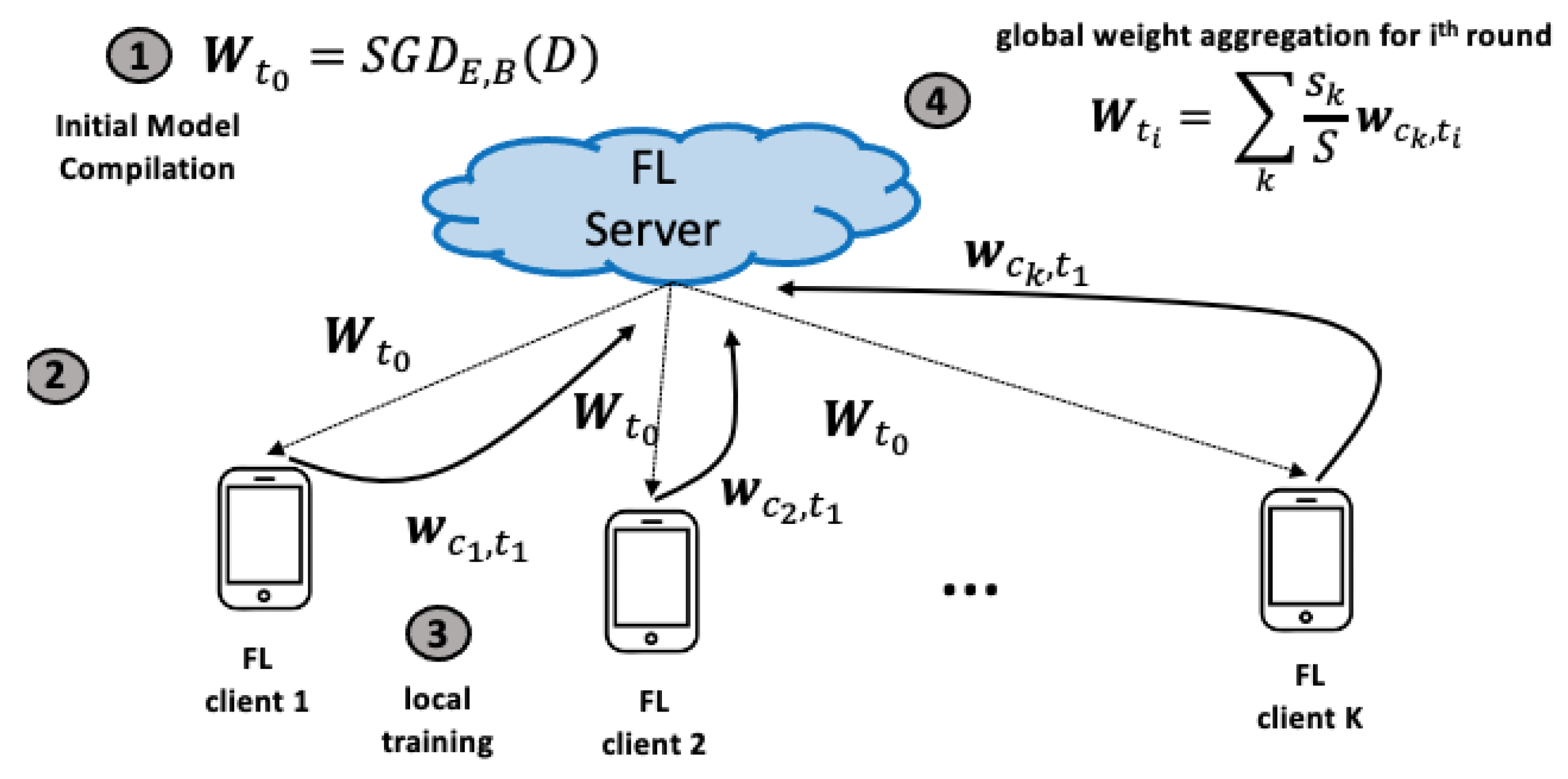
2. Background
| Algorithm 1 High-level and abstract overview of the FL model training paradigm |
|
3. Motivation
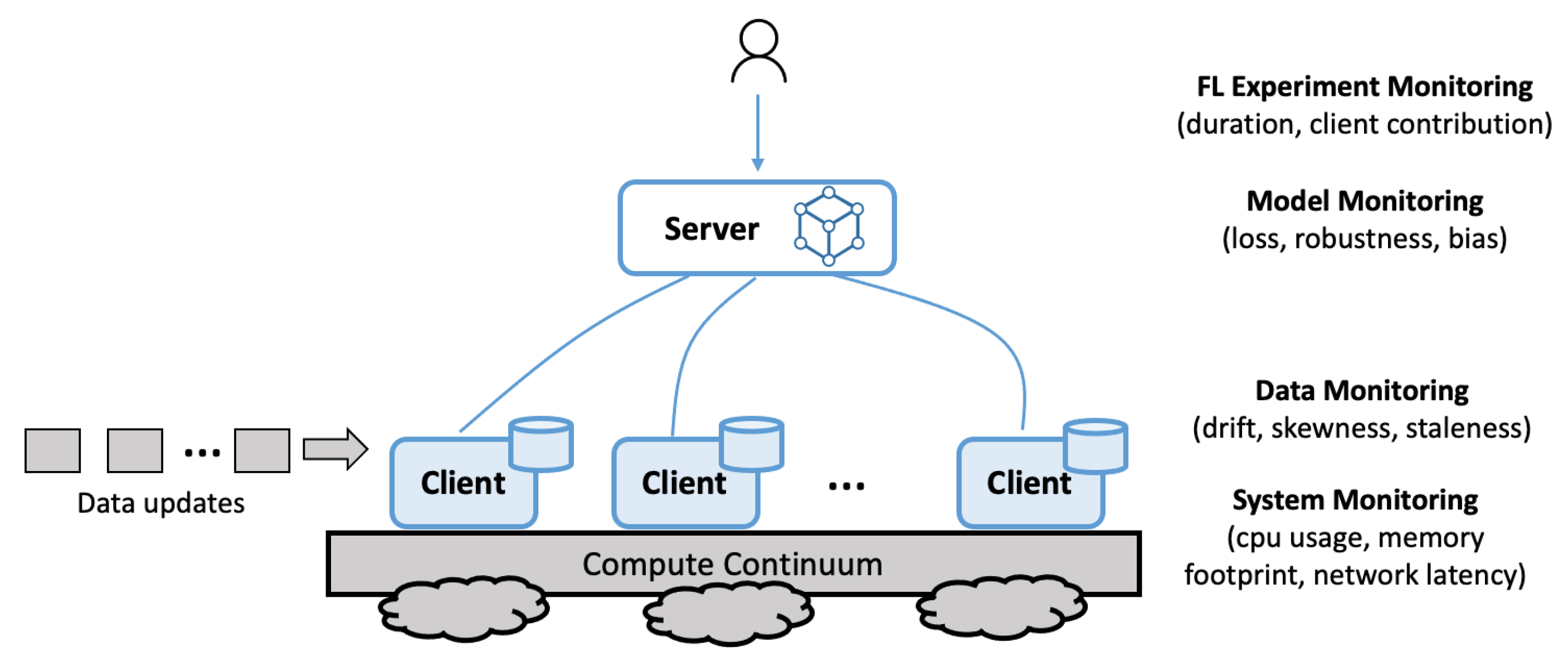
3.1. Challenge 1: Multi-Level Instrumentation
- The provisioned resources utility, including metrics such as CPU usage, memory footprint, and network latency.
- The input dataset, including metrics such as drift, skewness, and staleness, at both a local and global level.
- The output model, including metrics such as model loss, robustness, and bias with the reporting at a per-training-round level.
- Federated training run, including metrics such as the duration of the experiment, breakdown of training rounds and time, client contribution, costs, and failures.
3.2. Challenge 2: Training Round Temporal Granularity
3.3. Challenge 3: High Churn Rate
3.4. Challenge 4: Cross-Experiment Correlation
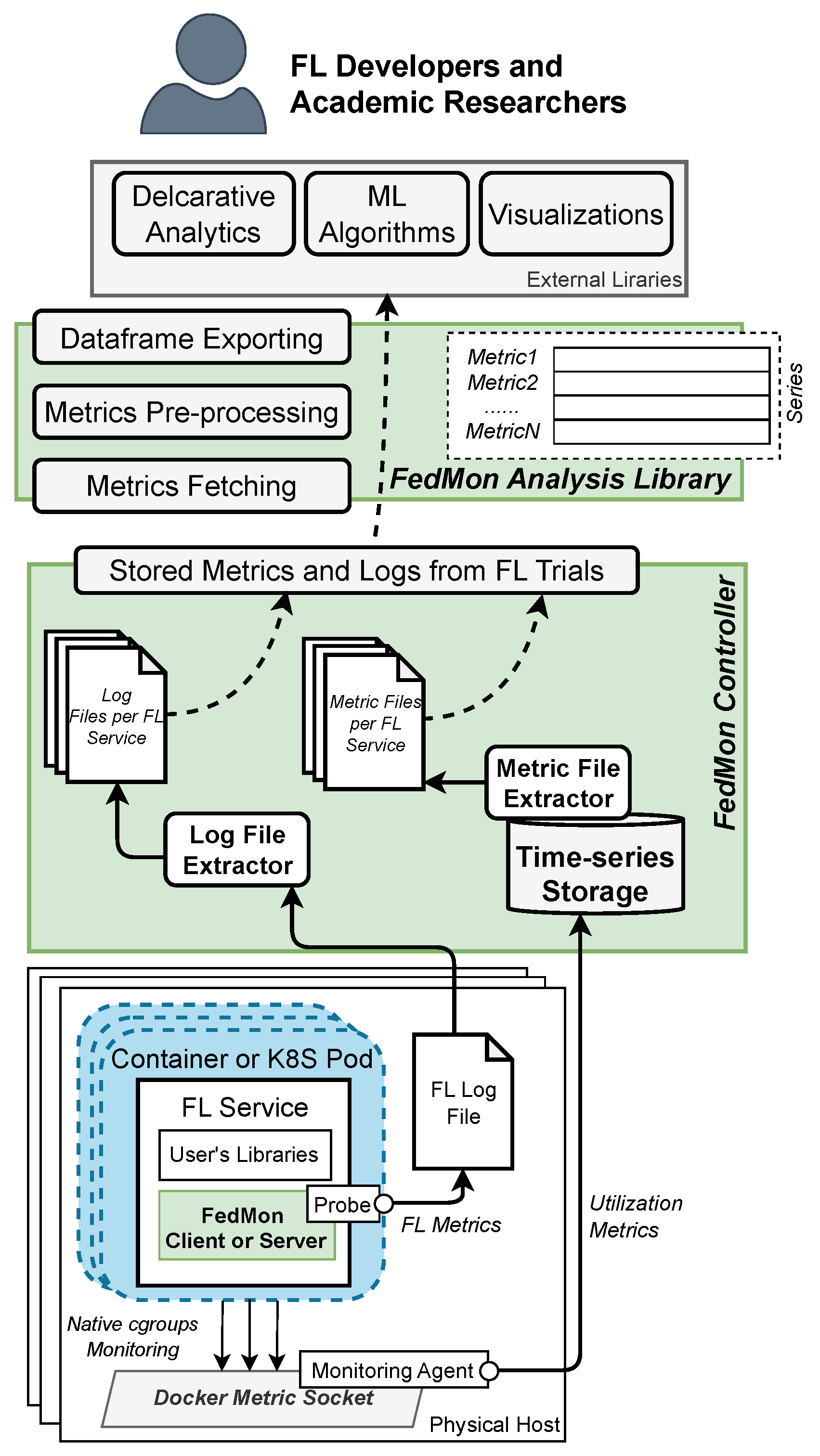
4. FedMon Framework Overview
5. Implementation Details
5.1. System Metrics and Monitoring Stack
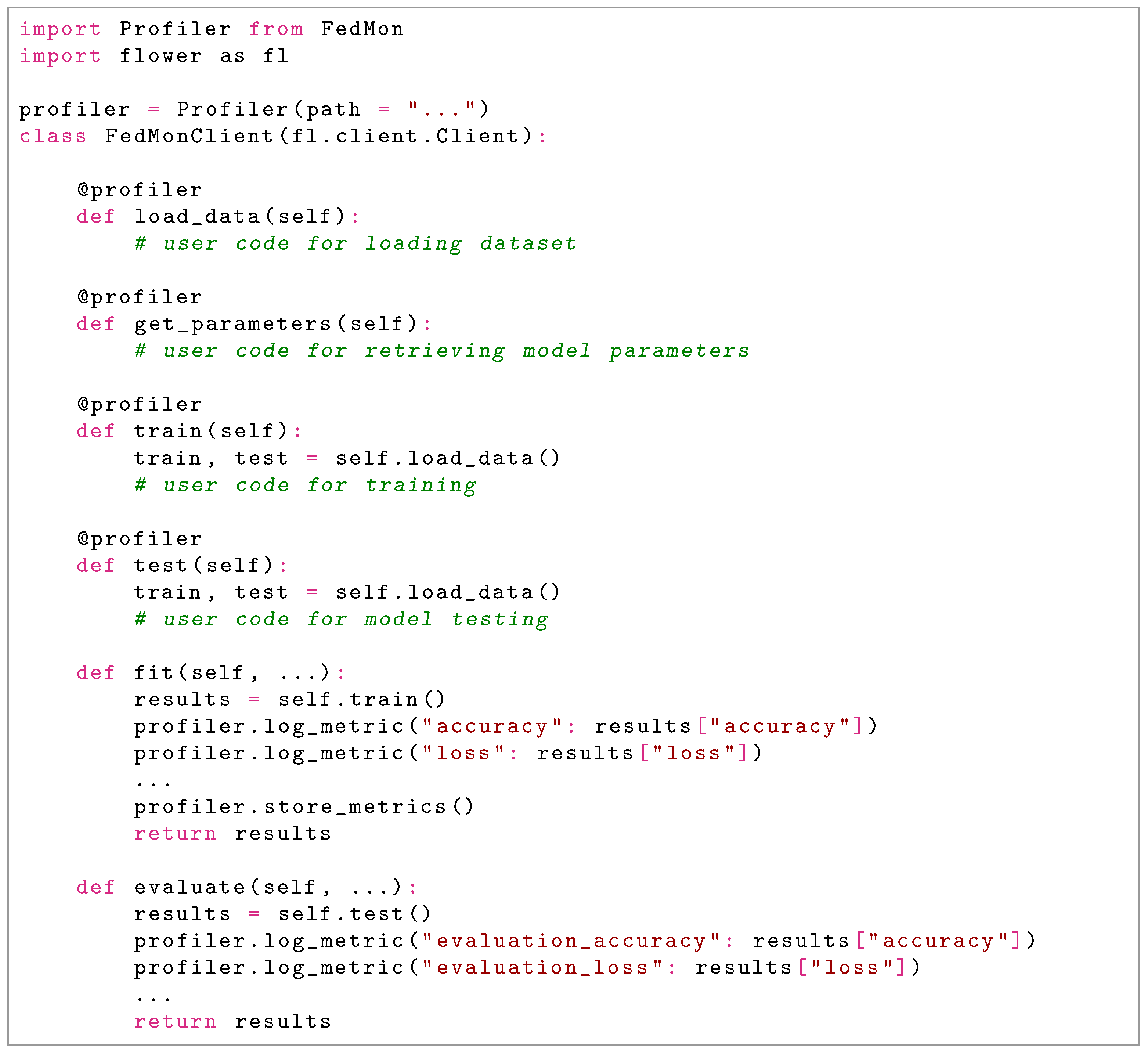
5.2. Client and Server FL Training Metrics
5.3. Metrics Analysis Library
5.4. User Interface
6. Experimentation
6.1. Use Case Overview
6.1.1. Description
6.1.2. Dataset
6.1.3. Models
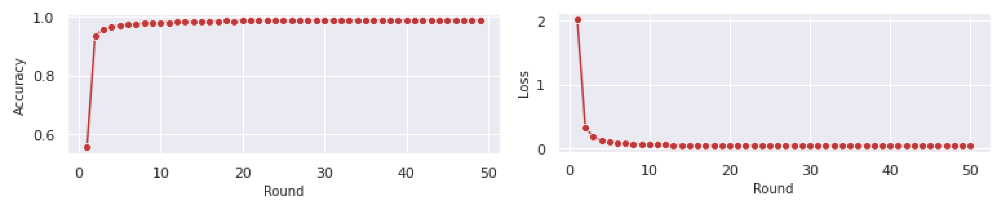
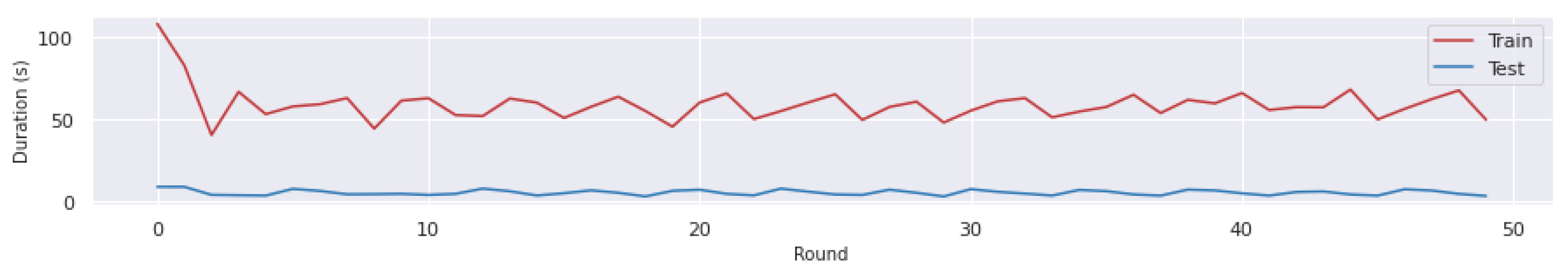
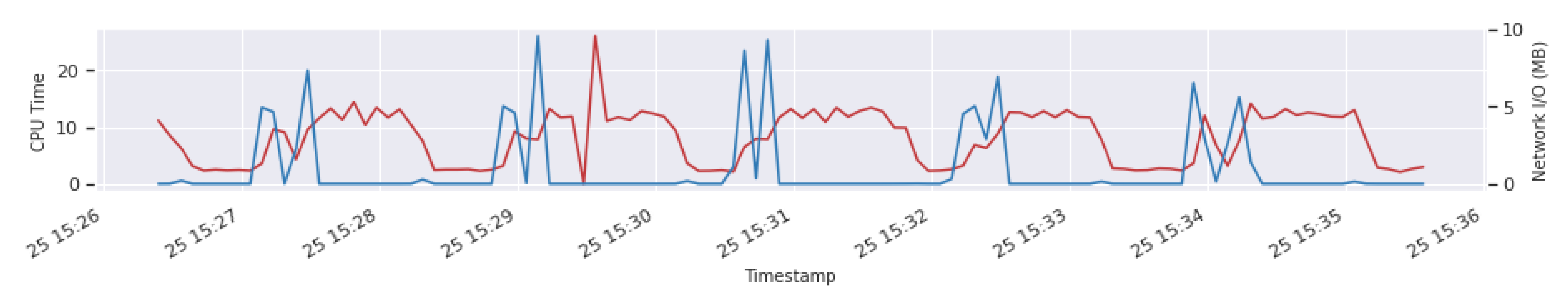
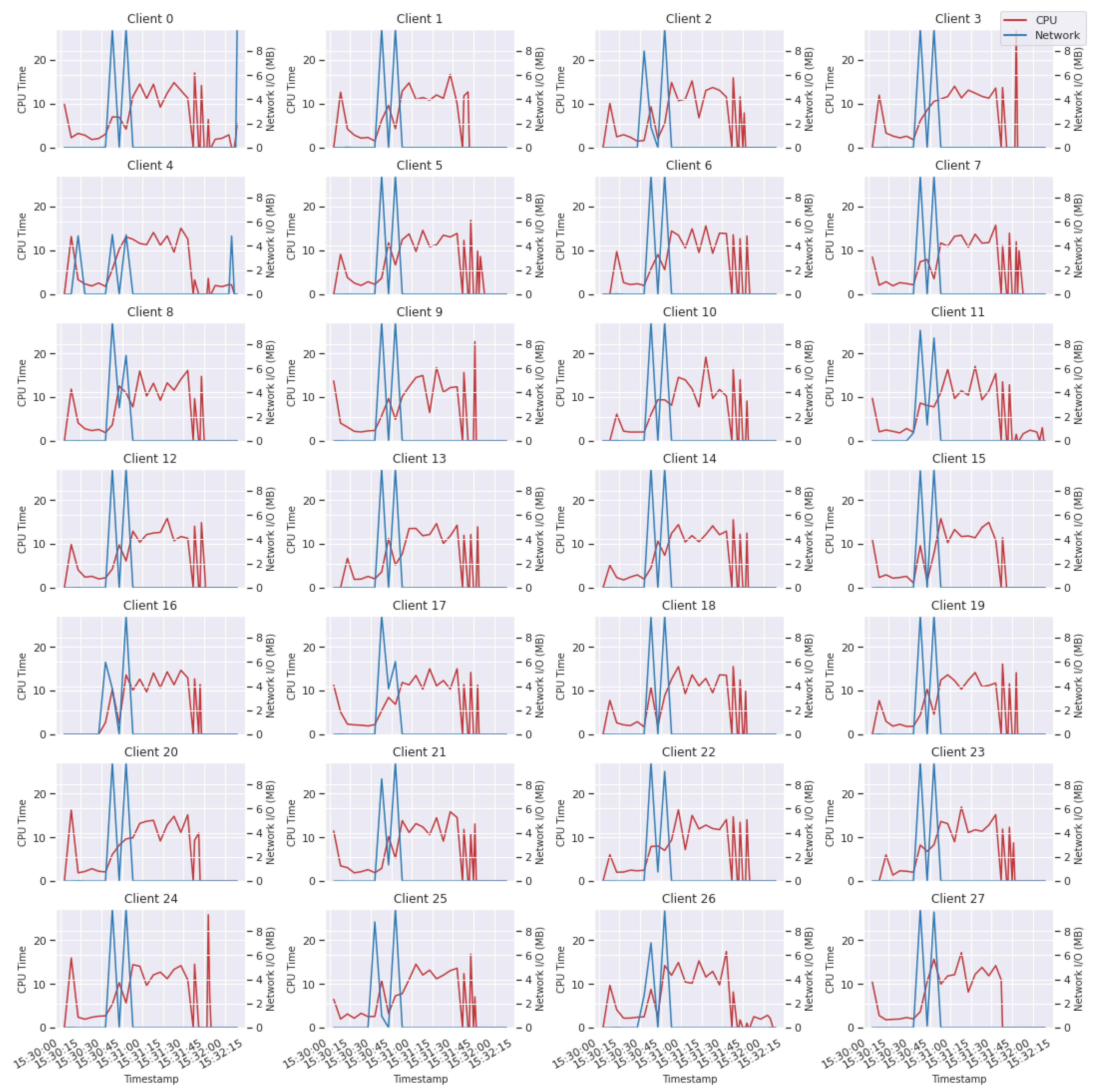
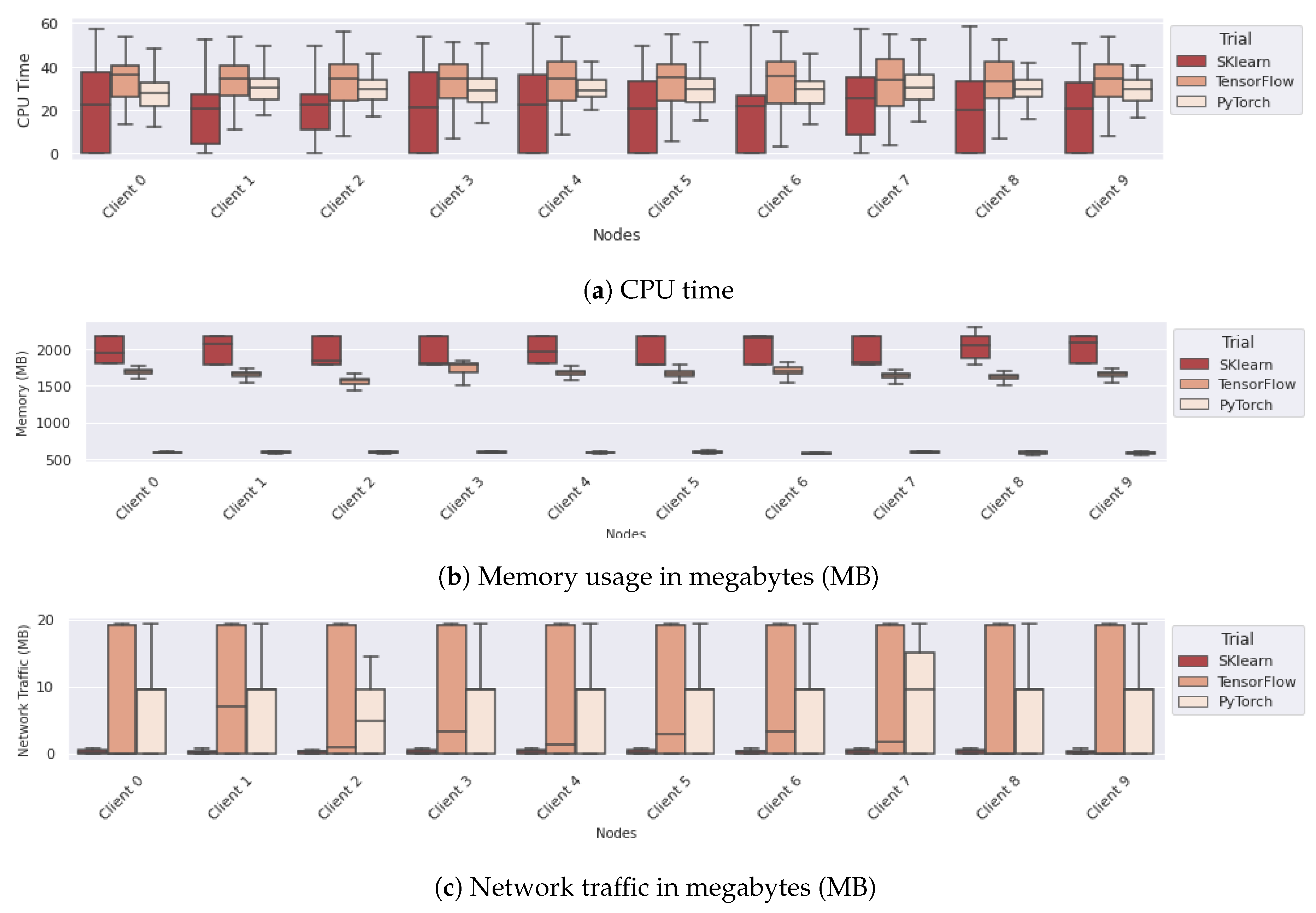
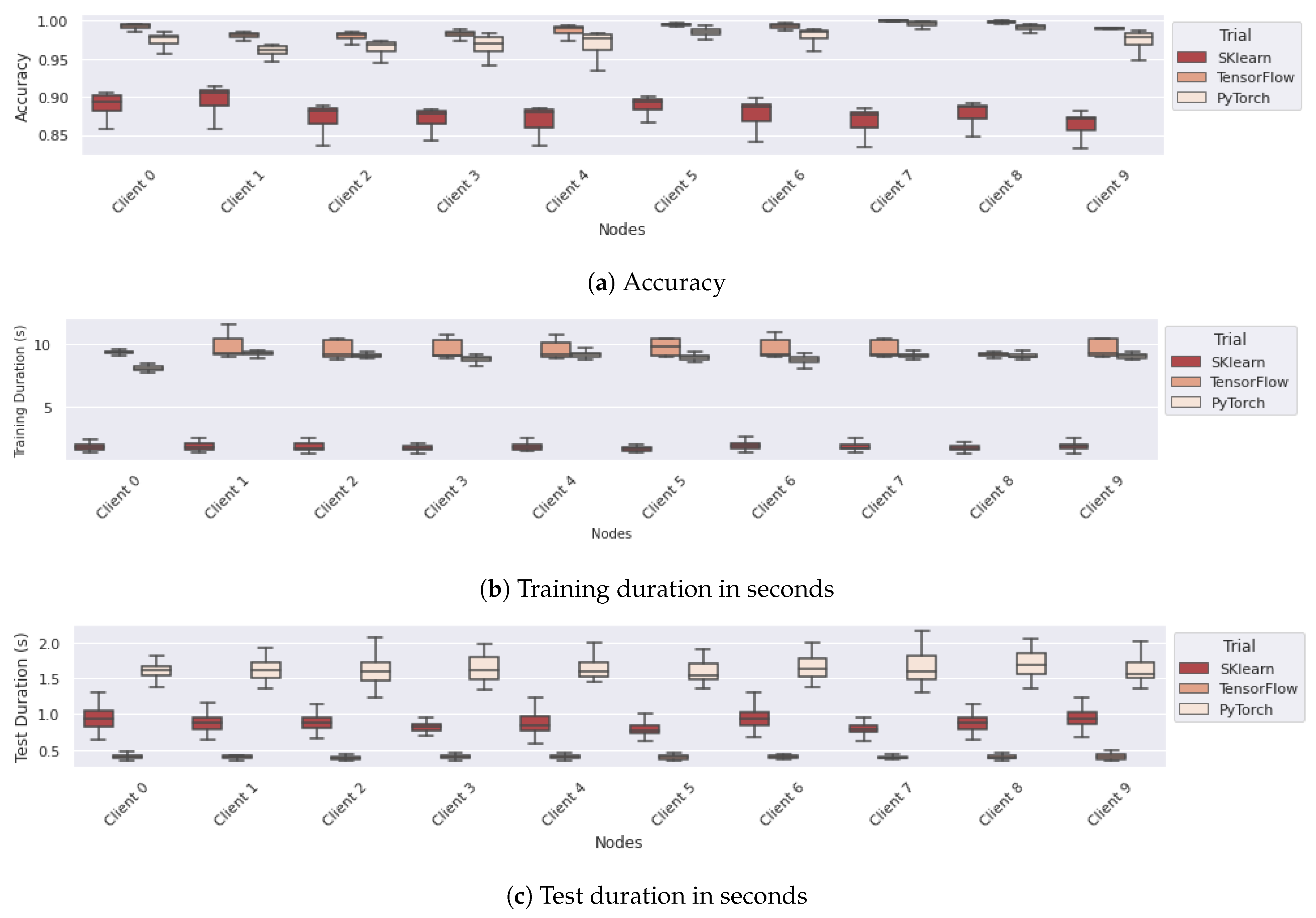
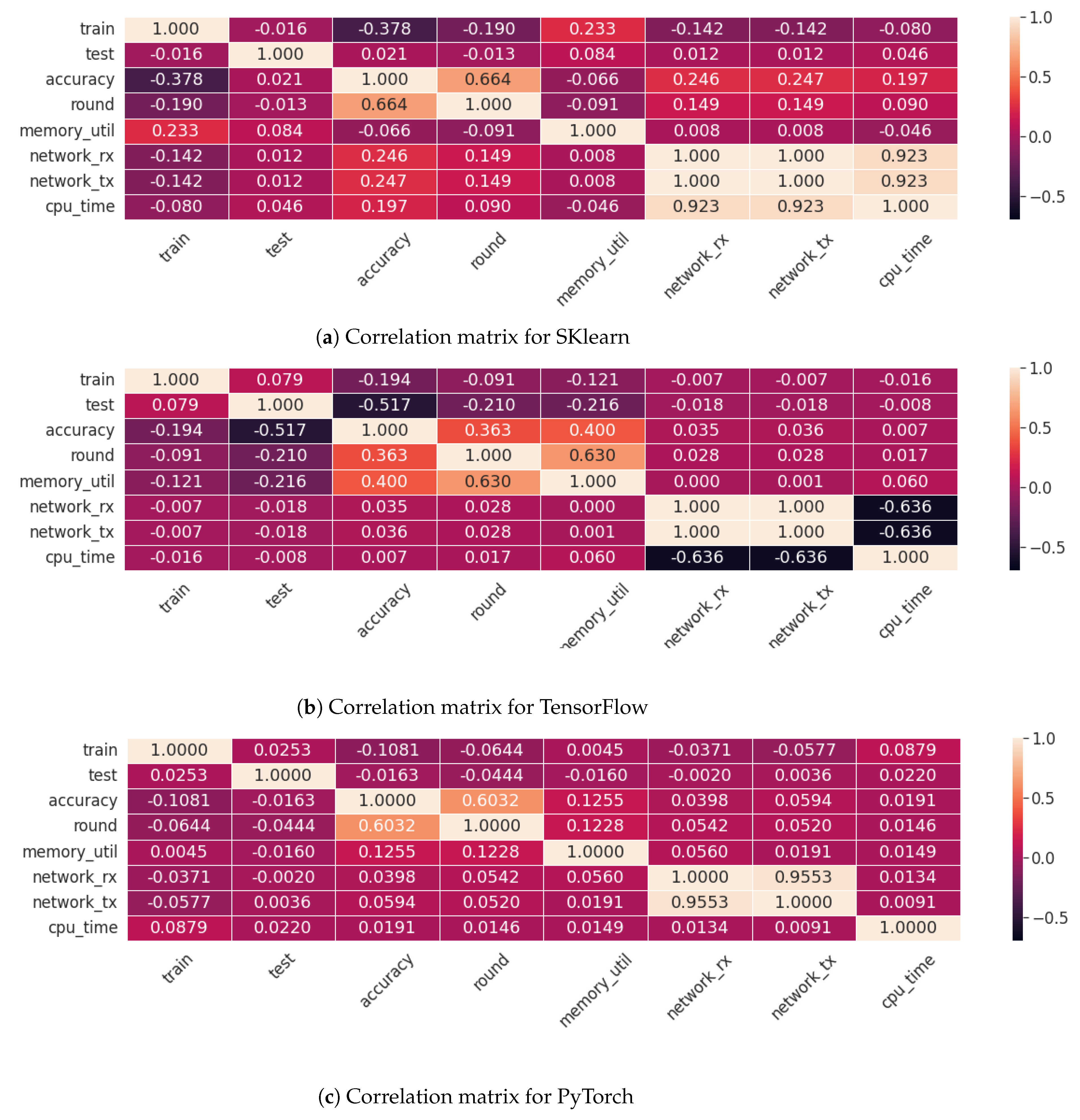
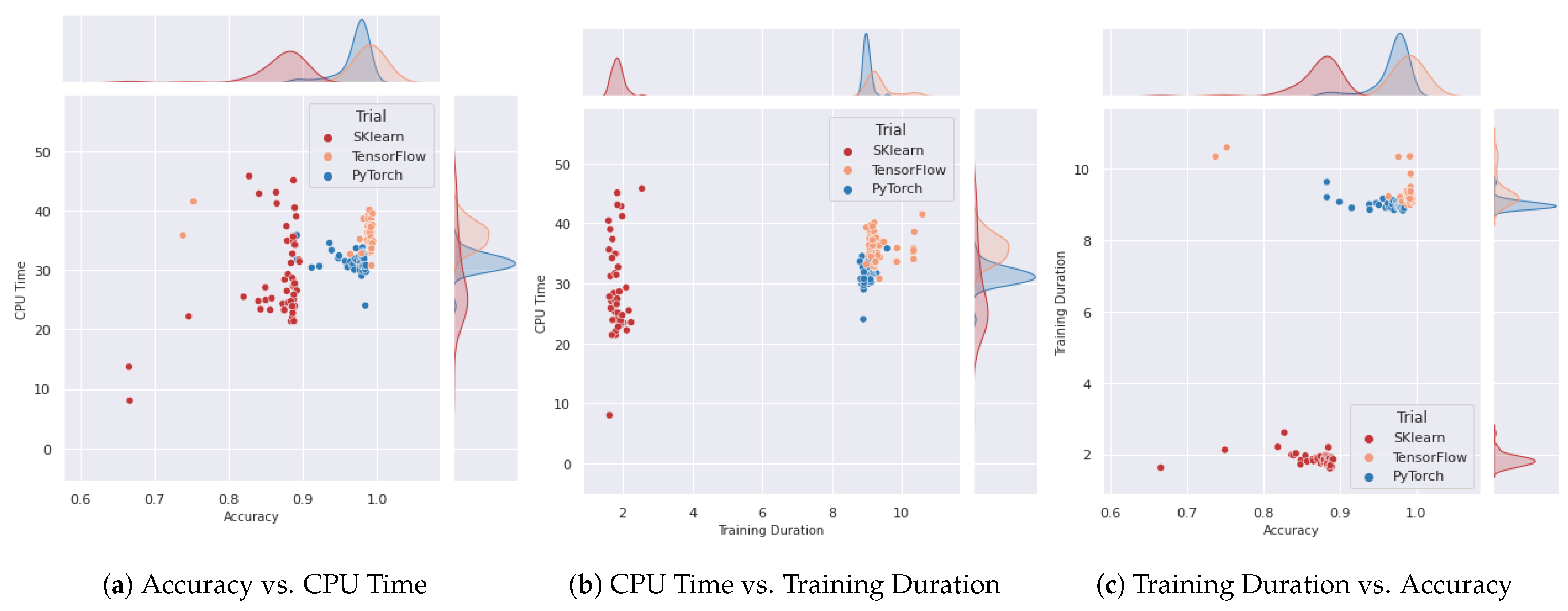
6.2. Exploratory Data Analysis
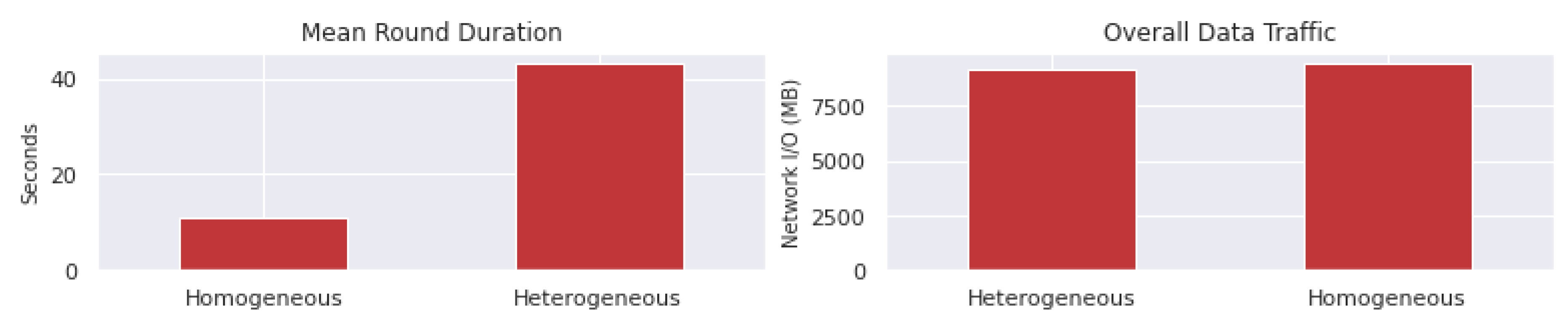
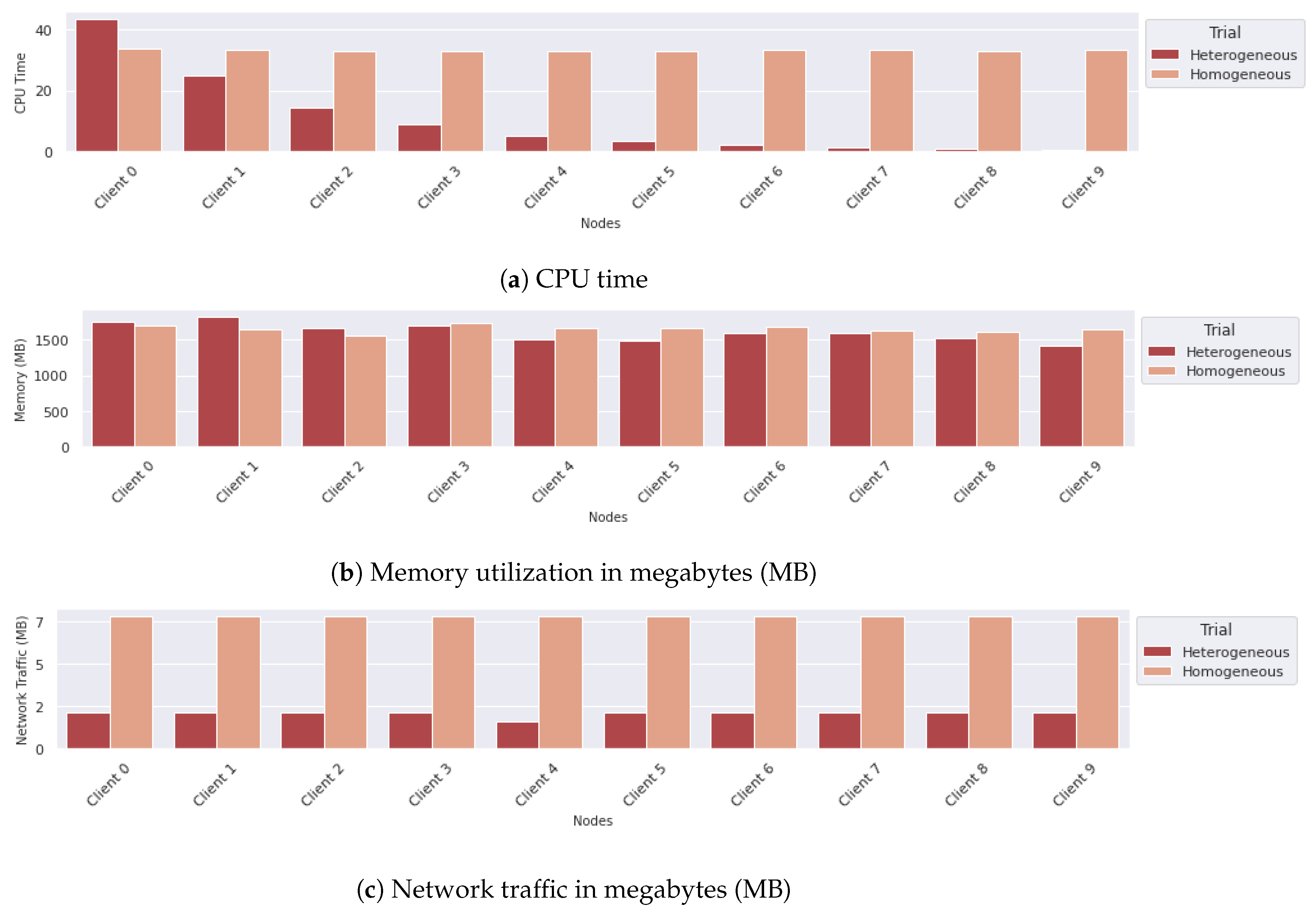
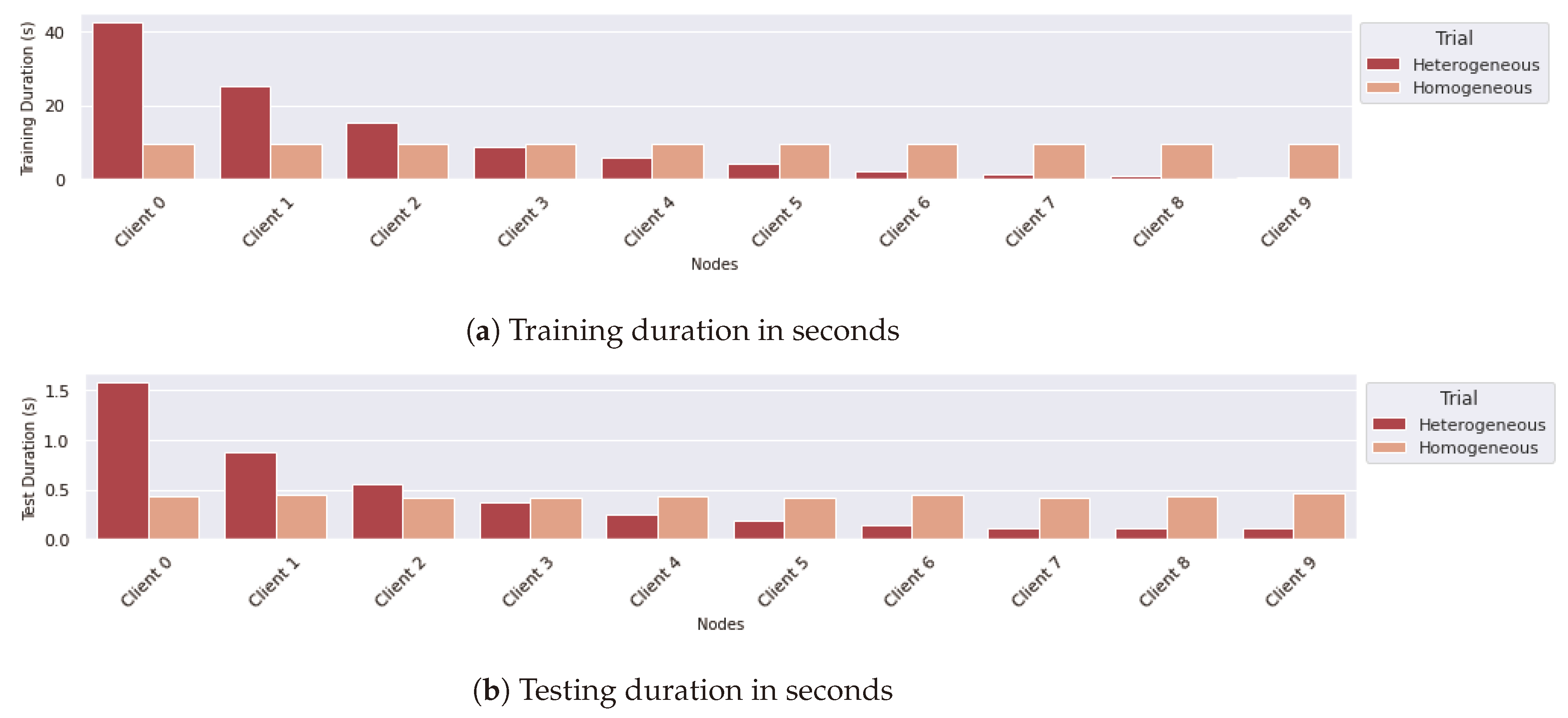
6.3. Comparing Different Configurations
6.4. Comparing Trials in Different Time Periods
7. Related Work
8. Conclusions and Future Directions
Author Contributions
Funding
Data Availability Statement
Conflicts of Interest
References
- Truong, N.; Sun, K.; Wang, S.; Guitton, F.; Guo, Y. Privacy preservation in federated learning: An insightful survey from the GDPR perspective. Comput. Secur. 2021, 110, 102402. [Google Scholar] [CrossRef]
- McMahan, B.; Moore, E.; Ramage, D.; Hampson, S.; Arcas, B.A.Y. Communication-Efficient Learning of Deep Networks from Decentralized Data. In Proceedings of the 20th AISTATS, PMLR, Fort Lauderdale, FL, USA, 20–22 April 2017; Volume 54, pp. 1273–1282. [Google Scholar]
- Li, T.; Sahu, A.K.; Zaheer, M.; Sanjabi, M.; Talwalkar, A.; Smith, V. Federated Optimization in Heterogeneous Networks. arXiv 2020, arXiv:1812.06127. [Google Scholar]
- Okegbile, S.D.; Cai, J.; Zheng, H.; Chen, J.; Yi, C. Differentially Private Federated Multi-Task Learning Framework for Enhancing Human-to-Virtual Connectivity in Human Digital Twin. IEEE J. Sel. Areas Commun. 2023, 41, 3533–3547. [Google Scholar] [CrossRef]
- Gadekallu, T.R.; Pham, Q.V.; Huynh-The, T.; Bhattacharya, S.; Maddikunta, P.K.R.; Liyanage, M. Federated Learning for Big Data: A Survey on Opportunities, Applications, and Future Directions. arXiv 2021, arXiv:2110.04160. [Google Scholar]
- Nikolaidis, F.; Symeonides, M.; Trihinas, D. Towards Efficient Resource Allocation for Federated Learning in Virtualized Managed Environments. Future Internet 2023, 15, 261. [Google Scholar] [CrossRef]
- Beutel, D.J.; Topal, T.; Mathur, A.; Qiu, X.; Fernandez-Marques, J.; Gao, Y.; Sani, L.; Li, K.H.; Parcollet, T.; de Gusmão, P.P.B.; et al. Flower: A Friendly Federated Learning Research Framework. arXiv 2022, arXiv:2007.14390. [Google Scholar]
- Foley, P.; Sheller, M.J.; Edwards, B.; Pati, S.; Riviera, W.; Sharma, M.; Narayana Moorthy, P.; Wang, S.H.; Martin, J.; Mirhaji, P.; et al. OpenFL: The open federated learning library. Phys. Med. Biol. 2022, 67, 214001. [Google Scholar] [CrossRef]
- Liu, Y.; Fan, T.; Chen, T.; Xu, Q.; Yang, Q. FATE: An Industrial Grade Platform for Collaborative Learning with Data Protection. J. Mach. Learn. Res. 2021, 22, 1–6. [Google Scholar]
- Symeonides, M.; Nikolaidis, F.; Trihinas, D.; Pallis, G.; Dikaiakos, M.D.; Bilas, A. FedBed: Benchmarking Federated Learning over Virtualized Edge Testbeds. In Proceedings of the 2023 IEEE/ACM 16th International Conference on Utility and Cloud Computing (UCC), Taormina, Italy, 4–7 December 2023. [Google Scholar]
- Trihinas, D.; Pallis, G.; Dikaiakos, M.D. Monitoring Elastically Adaptive Multi-Cloud Services. IEEE Trans. Cloud Comput. 2018, 6, 800–814. [Google Scholar] [CrossRef]
- Mallah, R.A.; Badu-Marfo, G.; Farooq, B. On the Initial Behavior Monitoring Issues in Federated Learning. IEEE Access 2021, 9, 161046–161054. [Google Scholar] [CrossRef]
- Sculley, D.; Holt, G.; Golovin, D.; Davydov, E.; Phillips, T.; Ebner, D.; Chaudhary, V.; Young, M. Machine Learning: The High Interest Credit Card of Technical Debt. In Proceedings of the SE4ML: Software Engineering for Machine Learning (NIPS 2014 Workshop), Montreal, QC, Canada, 13 December 2014. [Google Scholar]
- Breck, E.; Zinkevich, M.; Polyzotis, N.; Whang, S.; Roy, S. Data Validation for Machine Learning. In Proceedings of the SysML, Stanford, CA, USA, 31 March–2 April 2019. [Google Scholar]
- Netdata. 2024. Available online: https://www.netdata.cloud/ (accessed on 1 April 2024).
- Zavala, E.; Franch, X.; Marco, J. Adaptive monitoring: A systematic mapping. Inf. Softw. Technol. 2019, 105, 161–189. [Google Scholar] [CrossRef]
- Vartak, M.; Madden, S. Modeldb: Opportunities and challenges in managing machine learning models. IEEE Data Eng. Bull. 2018, 41, 16–25. [Google Scholar]
- Cho, Y.J.; Wang, J.; Joshi, G. Client Selection in Federated Learning: Convergence Analysis and Power-of-Choice Selection Strategies. arXiv 2020, arXiv:2010.01243. [Google Scholar]
- Jothimurugesan, E.; Hsieh, K.; Wang, J.; Joshi, G.; Gibbons, P.B. Federated learning under distributed concept drift. In Proceedings of the International Conference on Artificial Intelligence and Statistics, PMLR, Valencia, Spain, 25–27 April 2023; pp. 5834–5853. [Google Scholar]
- Mulay, A.; Gaspard, B.; Naidu, R.; Gonzalez-Toral, S.; Vineeth, S.; Semwal, T.; Manish Agrawal, A. FedPerf: A Practitioners’ Guide to Performance of Federated Learning Algorithms. Proc. Mach. Learn. Res. 2021, 148, 302–324. [Google Scholar]
- Prometheus. 2024. Available online: https://prometheus.io/ (accessed on 1 April 2024).
- cAdvisor. 2024. Available online: https://github.com/google/cadvisor (accessed on 1 April 2024).
- Symeonides, M.; Georgiou, Z.; Trihinas, D.; Pallis, G.; Dikaiakos, M.D. Fogify: A Fog Computing Emulation Framework. In Proceedings of the IEEE/ACM SEC, San Jose, CA, USA, 12–14 November 2020; pp. 42–54. [Google Scholar]
- Asad, M.; Shaukat, S.; Javanmardi, E.; Nakazato, J.; Bao, N.; Tsukada, M. Secure and Efficient Blockchain-Based Federated Learning Approach for VANETs. IEEE Internet Things J. 2024, 11, 9047–9055. [Google Scholar] [CrossRef]
- Nazir, S.; Kaleem, M. Federated Learning for Medical Image Analysis with Deep Neural Networks. Diagnostics 2023, 13, 1532. [Google Scholar] [CrossRef] [PubMed]
- Verginadis, Y. A Review of Monitoring Probes for Cloud Computing Continuum. In Proceedings of the International Conference on Advanced Information Networking and Applications, Juiz de Fora, Brazil, 29–31 March 2023; Barolli, L., Ed.; Springer: Cham, Switzerland, 2023; pp. 631–643. [Google Scholar]
- Nagios. 2024. Available online: https://www.nagios.com/ (accessed on 1 April 2024).
- Zabbix. 2024. Available online: https://www.zabbix.com/ (accessed on 1 April 2024).
- Ganglia. 2024. Available online: http://ganglia.info (accessed on 1 April 2024).
- Datadog. 2024. Available online: https://www.datadoghq.com/ (accessed on 1 April 2024).
- AppDynamics. 2024. Available online: https://www.appdynamics.com/ (accessed on 1 April 2024).
- Kashansky, V.; Kimovski, D.; Prodan, R.; Agrawal, P.; Marozzo, F.; Iuhasz, G.; Marozzo, M.; Garcia-Blas, J. M3AT: Monitoring Agents Assignment Model for Data-Intensive Applications. In Proceedings of the 2020 28th Euromicro International Conference on Parallel, Distributed and Network-Based Processing (PDP), Västerås, Sweden, 11–13 March 2020; pp. 72–79. [Google Scholar] [CrossRef]
- Trihinas, D.; Pallis, G.; Dikaiakos, M. Low-Cost Adaptive Monitoring Techniques for the Internet of Things. IEEE Trans. Serv. Comput. 2018, 14, 487–501. [Google Scholar] [CrossRef]
- Pusztai, T.; Morichetta, A.; Pujol, V.C.; Dustdar, S.; Nastic, S.; Ding, X.; Vij, D.; Xiong, Y. Slo script: A novel language for implementing complex cloud-native elasticity-driven slos. In Proceedings of the 2021 IEEE International Conference on Web Services (ICWS), Virtual, 5–11 September 2021; pp. 21–31. [Google Scholar]
- Schröder, T.; Schulz, M. Monitoring machine learning models: A categorization of challenges and methods. Data Sci. Manag. 2022, 5, 105–116. [Google Scholar] [CrossRef]
- EvidentlyAI. 2024. Available online: https://www.evidentlyai.com/ml-in-production/model-monitoring (accessed on 1 April 2024).
- Amazon. 2023. Available online: https://aws.amazon.com/sagemaker/ (accessed on 1 April 2024).
- WhyLabs. 2024. Available online: https://whylabs.ai/ (accessed on 1 April 2024).
- Chorev, S.; Tannor, P.; Israel, D.B.; Bressler, N.; Gabbay, I.; Hutnik, N.; Liberman, J.; Perlmutter, M.; Romanyshyn, Y.; Rokach, L. Deepchecks: A Library for Testing and Validating Machine Learning Models and Data. arXiv 2022, arXiv:2203.08491. [Google Scholar]
- Sun, R.; Li, Y.; Shah, T.; Sham, R.W.H.; Szydlo, T.; Qian, B.; Thakker, D.; Ranjan, R. FedMSA: A Model Selection and Adaptation System for Federated Learning. Sensors 2022, 22, 7244. [Google Scholar] [CrossRef]
- Meng, L.; Wei, Y.; Pan, R.; Zhou, S.; Zhang, J.; Chen, W. VADAF: Visualization for Abnormal Client Detection and Analysis in Federated Learning. ACM Trans. Interact. Intell. Syst. 2021, 11, 26. [Google Scholar] [CrossRef]
- Lee, T.; Mun, H.; Lee, Y. A Federated Learning Monitoring Tool for Self-Driving Car Simulation (Student Abstract); AAAI Press: Washington, DC, USA, 2023. [Google Scholar] [CrossRef]
- Li, Q.; Wei, X.; Lin, H.; Liu, Y.; Chen, T.; Ma, X. Inspecting the Running Process of Horizontal Federated Learning via Visual Analytics. IEEE Trans. Vis. Comput. Graph. 2022, 28, 4085–4100. [Google Scholar] [CrossRef] [PubMed]
- Wang, X.; Chen, W.; Xia, J.; Wen, Z.; Zhu, R.; Schreck, T. HetVis: A Visual Analysis Approach for Identifying Data Heterogeneity in Horizontal Federated Learning. arXiv 2022, arXiv:2208.07491. [Google Scholar] [CrossRef] [PubMed]
- Fan, T. FATE-Board: The FATE Monitoring and Visualization Toolkit. 2018. Available online: https://github.com/FederatedAI/FATE-Board (accessed on 1 April 2024).


| Metric | Category | Description | Default Granularity |
|---|---|---|---|
| CPU Utilization | System-level | The CPU utilization of FL client or server | 5s (Configurable) |
| Memory Utilization | System-level | The memory utilization of FL client or server | 5s (Configurable) |
| Network I/O | System-level | The network data (both incoming and outgoing) of FL client or server in bytes | 5s (Configurable) |
| Accuracy | Model metric | The model accuracy overall or per client | Per round |
| Loss | Model metric | The model loss overall or per client | Per round |
| Model Size | Model metric | Number of parameters and size in MB of them for the model | Per round |
| Round Duration | Experiment metric | The overall round duration and per client | Per round |
| Training Duration | Experiment metric | The training duration per round and per client | Per round |
| Testing Duration | Experiment metric | The testing duration per round and per client | Per round |
| Overall Duration | Experiment metric | The overall FL duration | Per experiment |
| Load Data Duration | Dataset metric | Data loading duration per round and per client | Per round |
| Data Size | Dataset metric | The size of the client’s dataset portion | Per experiment |
Disclaimer/Publisher’s Note: The statements, opinions and data contained in all publications are solely those of the individual author(s) and contributor(s) and not of MDPI and/or the editor(s). MDPI and/or the editor(s) disclaim responsibility for any injury to people or property resulting from any ideas, methods, instructions or products referred to in the content. |
© 2024 by the authors. Licensee MDPI, Basel, Switzerland. This article is an open access article distributed under the terms and conditions of the Creative Commons Attribution (CC BY) license (https://creativecommons.org/licenses/by/4.0/).
Share and Cite
Symeonides, M.; Trihinas, D.; Nikolaidis, F. FedMon: A Federated Learning Monitoring Toolkit. IoT 2024, 5, 227-249. https://doi.org/10.3390/iot5020012
Symeonides M, Trihinas D, Nikolaidis F. FedMon: A Federated Learning Monitoring Toolkit. IoT. 2024; 5(2):227-249. https://doi.org/10.3390/iot5020012
Chicago/Turabian StyleSymeonides, Moysis, Demetris Trihinas, and Fotis Nikolaidis. 2024. "FedMon: A Federated Learning Monitoring Toolkit" IoT 5, no. 2: 227-249. https://doi.org/10.3390/iot5020012
APA StyleSymeonides, M., Trihinas, D., & Nikolaidis, F. (2024). FedMon: A Federated Learning Monitoring Toolkit. IoT, 5(2), 227-249. https://doi.org/10.3390/iot5020012