1. Introduction
The knowledge and understanding of surface and deeper ocean dynamics, climate dynamics, and interactions between the oceans and atmosphere rely in quantitative observations and measurements, which have been increasing over time, most specifically due to recent observational capabilities, driven by technological advances in measuring systems, and are of key importance for ocean research, forecasting, and the services and management of sustainable development.
Despite global-scale autonomous and satellite measurements having started in the 1970s [
1], and even if, nowadays, remote sensing and numerical modelling are important for ocean-related research, the fact is that, for example, satellite remote sensing observations just deliver data from the surface layers of the ocean, and around 98.8% of the ocean volume remains unobservable [
2], and numerical models provide most of the derived and predicted data [
3]. Consequently, both approaches need to be complemented by key high-quality in situ measurements, which ships still provide from their ocean-wide observations, delivering calibration and context for developmental, autonomous, and satellite measurements, as well as for initialization, validation, or assimilation [
1,
3].
Ocean studies require continuous monitoring, and there is an increasing need to perform ocean observations reliably and in a cost-effective manner, ensuring high density in space and time [
2]. Nowadays, oceanographic research vessels play a crucial role in conducting a wide spectrum of observations encompassing atmospheric, oceanographic, chemical, biological, and other parameters. However, constrained by limited budgets, research vessels often face challenges in maintaining regular and systematic observations at specific locations, leading to potential seasonal and spatial biases. High-latitude areas are infrequently visited during wintertime [
4]. In contrast, conventional vessels traverse the oceans under adverse weather conditions, often navigating inhospitable waters. For example, commercial vessels adhere to traditional ocean routes, facilitating the repetition of observations in specific local regions and contributing to extensive time series data; fishing vessels, operating in coastal seas all year-round and under almost all-weather conditions [
3], are able to contribute with crucial data, even in unfavourable weather and remote regions. So, whether commercial or otherwise, these vessels may function as versatile sampling platforms, providing valuable insights into biological, physical, chemical, and geological ocean parameters, and they are called vessels of opportunity (VOO).
The use of VOO is a complementary alternative for long-term and spatially wide-spread sustainable scientific measurements and can comprehend merchant and research vessels, fishing vessels, cruise liners, ferries, military vessels, and yachts, among others [
4].
The ultimate success of VOO observing systems relies, at its final stage, on the quality of data generated and subsequently made accessible to end users through databases. This, in turn, strongly depends on the initial design of the measuring system, installed on each of the VOO.
The use of self-contained, low-maintenance sensor systems installed in VOO is progressively emerging as a vital scientific tool across various global regions. These systems usually integrate data from meteorologic and oceanographic data sensors, along with global navigation satellite system (GNSS) data, often transmitted in real-time from the vessel to onshore facilities. The data collected serve diverse purposes, encompassing safety navigation conditions, the selection of optimized routes for both safety and economic considerations, and scientific research objectives.
While there have been numerous successful implementations of these observing systems in VOO (e.g., [
3]), their integration still poses challenges. This is attributed not only to the distinct configurations of each vessel but also to the specific requirements of the systems, which include the proper installation of measuring devices, the operational conditions, sensor calibration, and the use of appropriate data communication platforms.
Moreover, there is still a need to improve instrument technology for autonomous sampling, particularly for the cloud cover, cloud type, and sea state [
4].
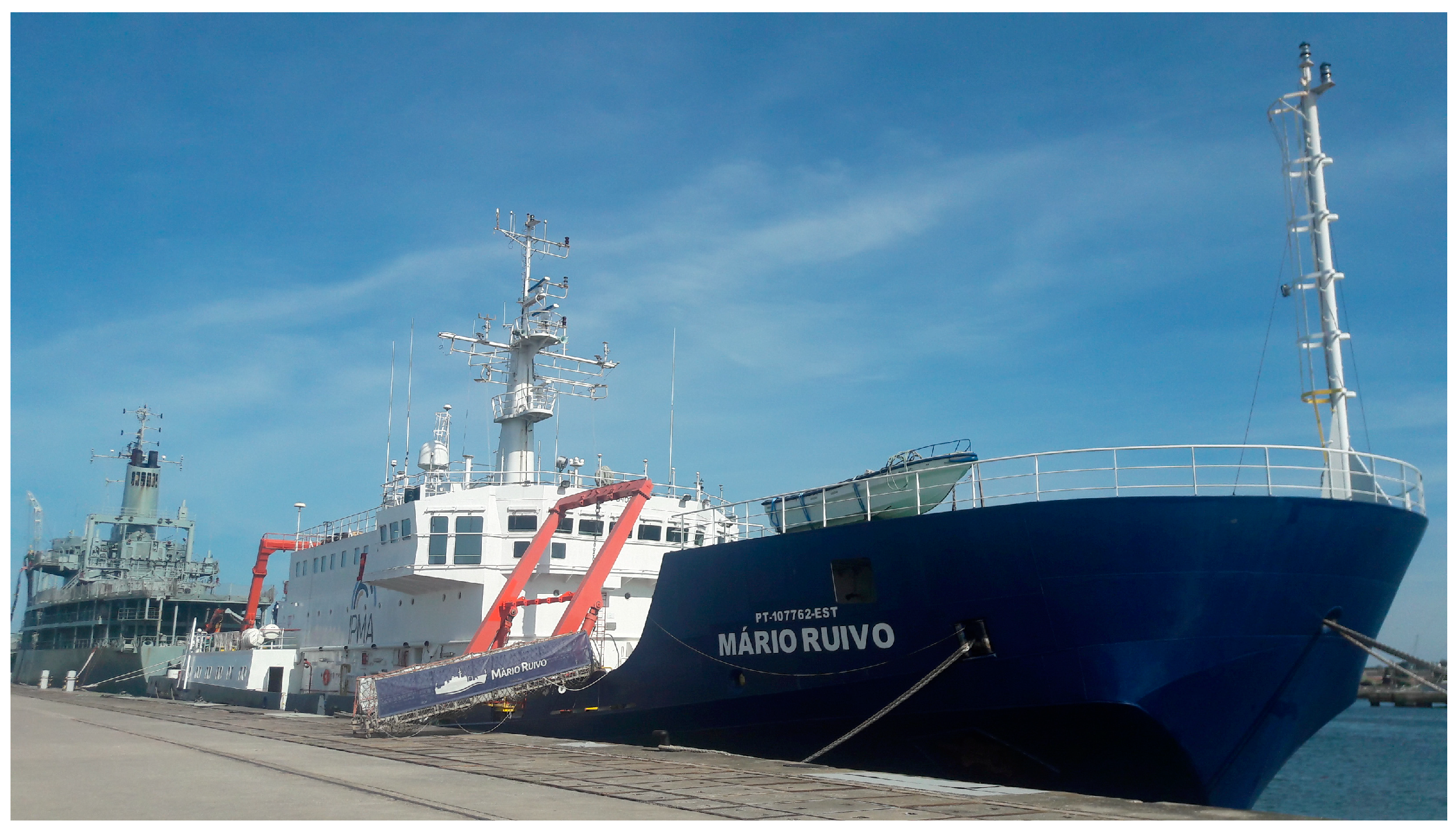
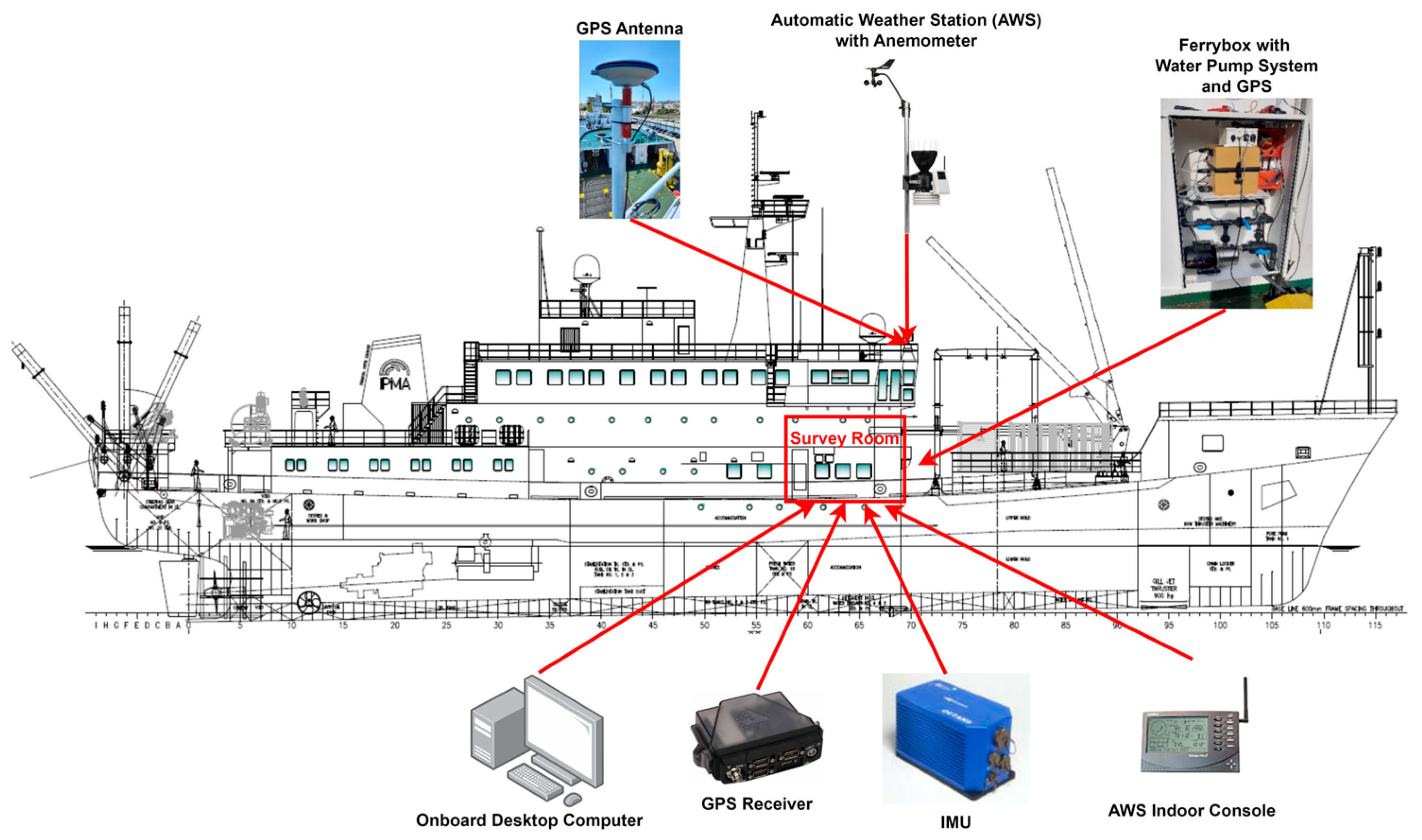
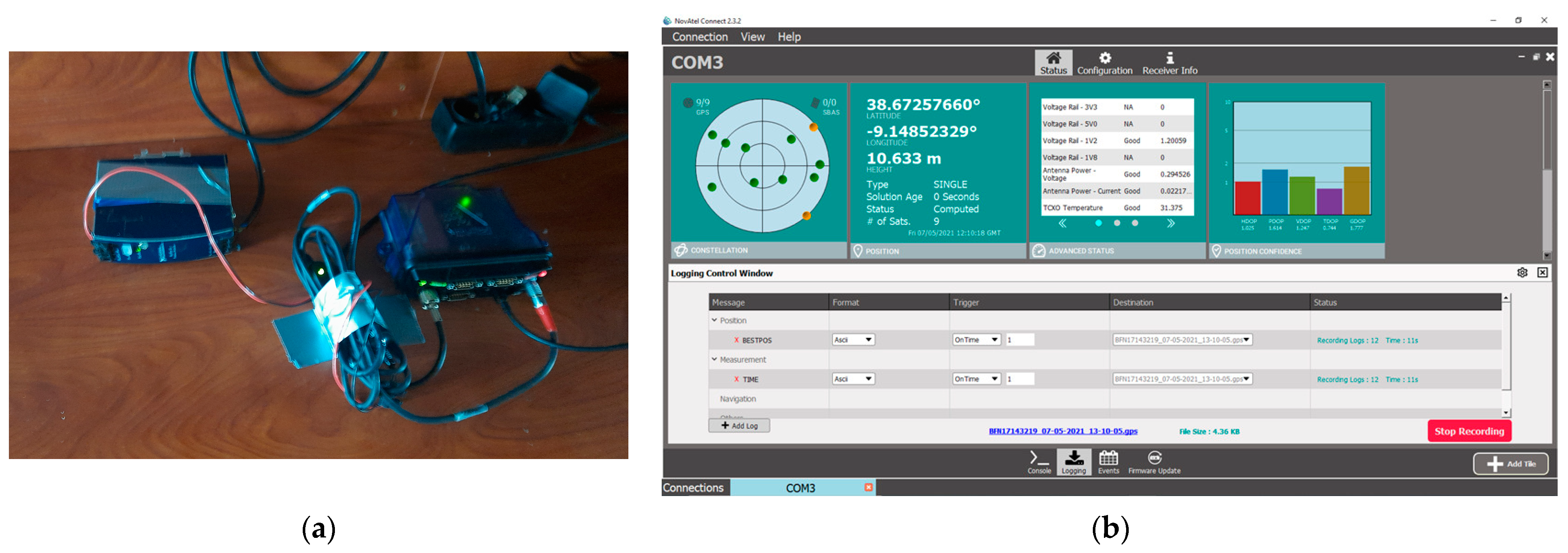
The present paper describes the main key components of an autonomous observation system (AOS) prototype installed onboard a Portuguese research vessel, along with its outcomes observed during a sea full-scale trial. It consists of underway measurements of air temperature and humidity, barometric pressure, and wind speed and direction from an automatic weather station (AWS); sea water temperature, pH, dissolved oxygen, total dissolved solids (TDS), salinity, conductivity, turbidity, chlorophyll-a, and phycocyanin from a Ferrybox coupled with a water pumping system; roll, pitch, heave, and yaw (true heading) from an inertial measurement unit (IMU); and geolocation from a global navigation satellite system (GNSS) unit.
By integrating AOS technology into VOO operations, this paper aims to demonstrate the feasibility and practicality of this approach for acquiring high-quality environmental data. This objective is achieved through the presentation of a prototype system that allows for the collecting and integration of meteorological and ocean data and was developed to be installed, in the near future, mainly in fishing vessels operating as VOO.
The characteristics of the prototype are fully described, and the primary focus is on the integrated atmospheric and wave information obtained during a full-scale trial, conducted in May 2021, on a research vessel operating as VOO. These data are analysed and discussed, considering both the advantages and limitations of the developed AOS, in order to provide potential future enhancements aimed at optimizing the system performance and functionality.
2. Brief Overview on AOS Initiatives
The initial scientific ocean observations were based on single-ship expeditions aiming to chart ocean geology, biology, chemistry, and circulation.
The period spanning the end of the nineteenth century to the onset of World War I (WWI) witnessed the first global ocean expeditions extending to high latitudes. Simultaneously, there was a substantial advancement in the study of ocean thermodynamics, with a specific focus on salinity, temperature, and density phenomena, alongside an evolution on the study of oceanic dynamics. Furthermore, there was notable progress in the understanding of fluid dynamics and atmospheric processes, which contributed to the enhancement of knowledge of the ocean–atmosphere interaction processes.
Following World War I, the 1920s and early 1930s witnessed a significant surge in oceanographic data collection, characterized by major expeditions covering all the oceans. These led to research outcomes which paved the way for mid-century developments in ocean dynamics. In turn, with World War II (WWII) came oceanographic explorations which relied on technologies and observing systems, such as ocean weather stations (OWSs), developed by navies to assist the aviation industry.
Within a decade, comprehensive surveys of the Atlantic and Pacific oceans, among others, were conducted, contributing significantly to the modernization of measurements and the understanding of ocean chemistry and biogeochemistry. Furthermore, substantial technological advancements were made in instrumentation. Regarding surface meteorology and air–sea fluxes, over the last 100 years, estimations have been based on observations made by commercial ships and surface buoys but also from research vessels and VOO.
Gridded surface meteorology and air–sea flux products have been derived from observations, numerical models, satellite observations, and a combination of all of these [
1].
Next, we describe several vessels of opportunity (VOO) initiatives, providing details on the employed observing systems whenever feasible.
The shipboard automated meteorological and oceanographic system (SAMOS) initiative collected, quality-evaluated, distributed and archived underway navigational, meteorological, and oceanographic observations sampled since 2005 at 1 min intervals from VOO research vessels operating in both coastal and open-ocean environments well out-side the shipping routes of merchant vessels. This initiative has been designed to answer the data needs within the air–sea interaction, satellite and remote sensing, numerical modelling, and geoscience informatics communities. The data have also been used to validate satellite data products and to define the set of conditions needed to develop new satellite retrieval algorithms [
5].
Each autonomous observing system (AOS) within the SAMOS project consists of fully automated instrumentation, such as a computerized data acquisition system, one or more pieces of navigational equipment, electronic meteorological instrumentation, and oceanographic sensors, providing measurements of a set of parameters, which include a subset of essential climate/ocean variables (ECV/EOVs). These devices are purchased, deployed, maintained, and operated by the research vessel home institution. Moreover, the observations’ data records follow a processing workflow from each VOO to the Marine Data Centre (MDC) at Florida State University, firstly being sent over via an e-mail protocol by an operator in the ship. Then, in the MDC, the files undergo two fully automated quality controls (QCs), and for selected vessels, a visual QC by a data-quality analyst is conducted. Preliminary, intermediate, and research-quality netCDF files are made available to users via the Web, for example [
5]. For instance, ref. [
6] uses several atmospheric and ocean variables, such as air temperature, sea-surface temperature, relative humidity, and wind speed from SAMOS netCDF files to calculate bulk turbulent heat and momentum fluxes. These SAMOS data come from a quality-controlled archive of underway observations from research vessels.
The International Comprehensive Ocean–Atmosphere Data Set (ICOADS) hosted by the United States National Oceanic and Atmospheric Administration (NOAA) stands out as one of the most extensive and diverse freely accessible archives of global surface marine data. It encompasses the evolution of measurement technology over the past three centuries, which, by the year 2017, had over 455 million individual marine reports, each containing surface meteorological observations and metadata reported from voluntary observing ships (VOSs), buoys, coastal platforms, or other in situ ocean data acquisition systems (ODASs). The ICOADS contains observations of many global climate observing system (GCOS) essential climate variables (ECVs) for both atmospheric and oceanic domains [
7].
The voluntary observing ship’s (VOS) scheme is the main program of the ship observations team (SOT) of the Joint Technical Commission for Oceanography and Marine Meteorology (JCOMM) of the World Meteorological Organization (WMO) and of the Inter-governmental Oceanographic Commission (IOC) of the United Nations Educational, Scientific, and Cultural Organization (UNESCO) [
8]. The VOS activities, i.e., the WMO marine activities and those of the IOC, have been coordinated since 1999 by the Observation Coordination Group (OCG) for the global ocean observing system (GOOS) [
9]. At the international level, these activities are undertaken through the JCOMM in situ of the Observing Programme Support (JCOMMOPS) Centre [
8]. The VOS scheme international program involves member countries of the WMO [
9], providing the governance by which ships are recruited by the National Meteorological and Hydrographic Services (NMHSs) for making, recording, and transmitting meteorological observations whilst at sea [
4,
9]. The most critical data are air pressure, wind speed and direction, sea state, humidity, visibility, and air and sea-surface temperature [
10]. For near real-time applications and once ashore, the observations are shared internationally with the users (e.g., meteorologists, numerical weather prediction models, ship routing services) through the WMO global telecommunication system (GTS) [
4,
8,
10].
This scheme involves a fleet of more than 3000 VOSs operating worldwide [
8]. The meteorological services of most maritime countries within the VOS scheme set agreements with ships regularly crossing their coasts to take and transmit marine meteorological observations to shore at no cost to the ships. By providing the instrumentation plus forecasting and warnings to ships, the meteorological services are generally provided with free-of-charge observations from the shipping companies [
11].
Presently, numerous observations are still taken manually and are subsequently inserted into an electronic logbook software (e.g., TurboWin+ V4.4, OBSJMA for WIN Version 3.00) which then calculates and corrects some variables (e.g., true wind, sea level pressure). This software can also perform quality control, coding data for immediate transmissions to shore, and format the observation for digitization. Many observations are sent via INMARSAT C. However, numerous NMHSs are increasingly equipping ships with an automatic weather station (AWS) that may either operate automatically or accept the manual input of visual parameters (clouds, weather, sea, and swell) entered into a computer [
11]. The advantage of AWS systems is the automation of the measurements and transmissions of several meteorological parameters by satellite at hourly intervals without the need for human intervention. Moreover, several tools have been developed to monitor the quantity, quality, and timeliness of the observational data, thus helping in identifying those ships whose data are of poorer quality, and consequently to take corrective measures to address observing errors or device calibration issues [
8].
The JCOMM is also responsible for the VOS Climate Fleet (VOSClim) program and Ships of Opportunity Program (SOOP). The VOSClim provides a high-quality subset of VOS data in real-time and delayed mode, supplemented by a broad set of metadata to support global climate studies and research. The VOSClim ships, like other VOS vessels, work with electronic logbook software, but they also input other variables such as the ship’s ground course and speed, the ship’s heading, the maximum height of the cargo above the summer load line, and the difference between the summer load line and the waterline. By adding information of the location of the instruments within the ship, researchers can model the wind flow over a ship. The fleet comprised more than 450 ships, as of 2015, reporting observations from world oceans. The SOOP is mainly dedicated to collecting oceanographic data, like upper ocean thermal (UOT) measurements and, from time to time, atmospheric and ocean carbon, fluorescence and pigments, subsurface temperature, and salinity data. The UOT measurements are made on the top 1000 m of the oceans by bathythermographs probes dropped mostly by volunteer ships, like merchant, research, and naval vessels [
10]. The SOOP has data management-related activities undertaken in collaboration with the Global Temperature–Salinity Profile Program (GTSPP), which is a joint program of the International Oceanographic Data and Information Exchange (IODE) committee and the JCOMM [
12].
4. Results of the Full-Scale Trial
In this section, the results related to the meteorological and wave and parameters are presented and analysed. The results derived from the Ferrybox system will be addressed in a forthcoming paper.
The meteorologic experimental results were obtained from the readings of the AWS. The true wind speed and direction estimates were derived from the anemometer data complemented by measurements from the motion sensor and GNSS units. These results were validated through a comparison with data obtained from a second set of sensors installed onboard the RV.
4.1. Meteorological Parameters
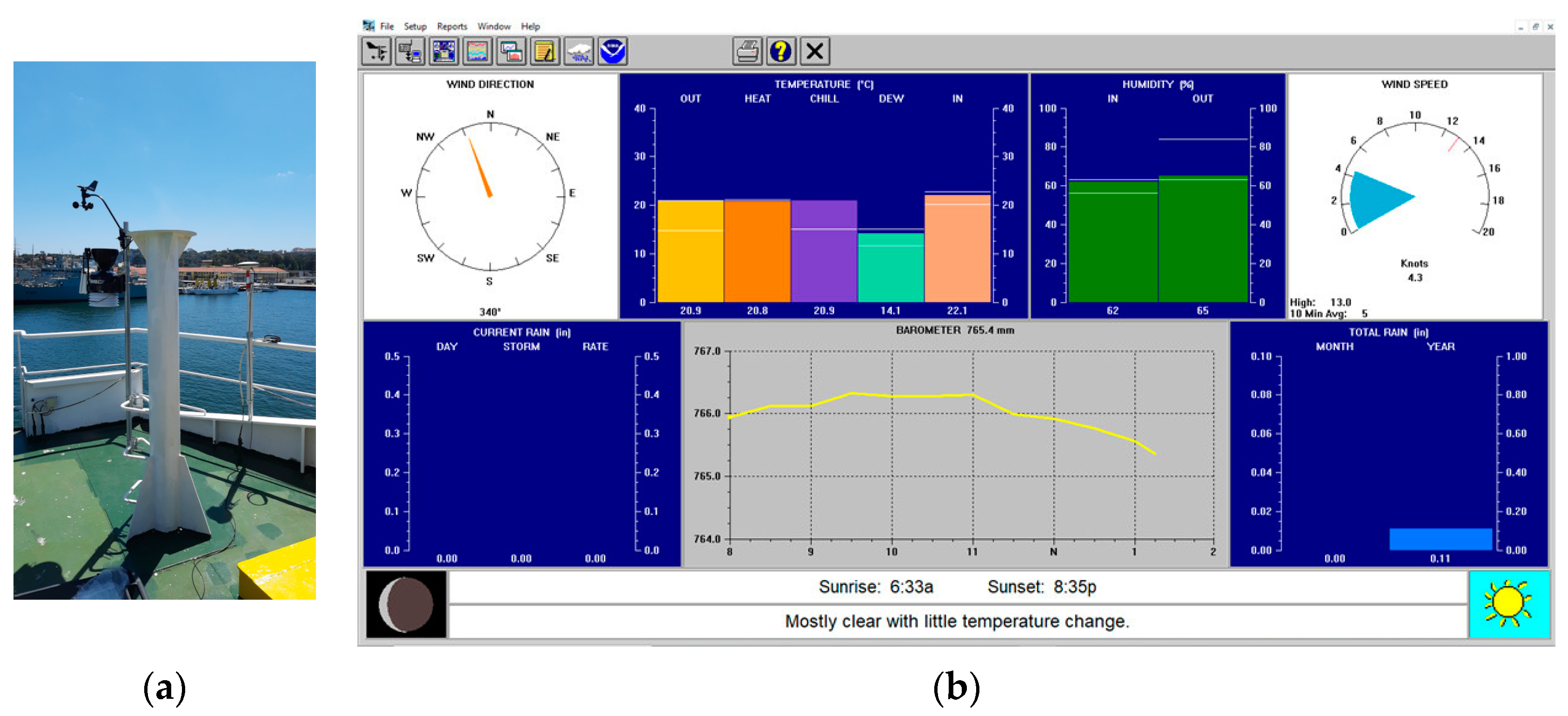
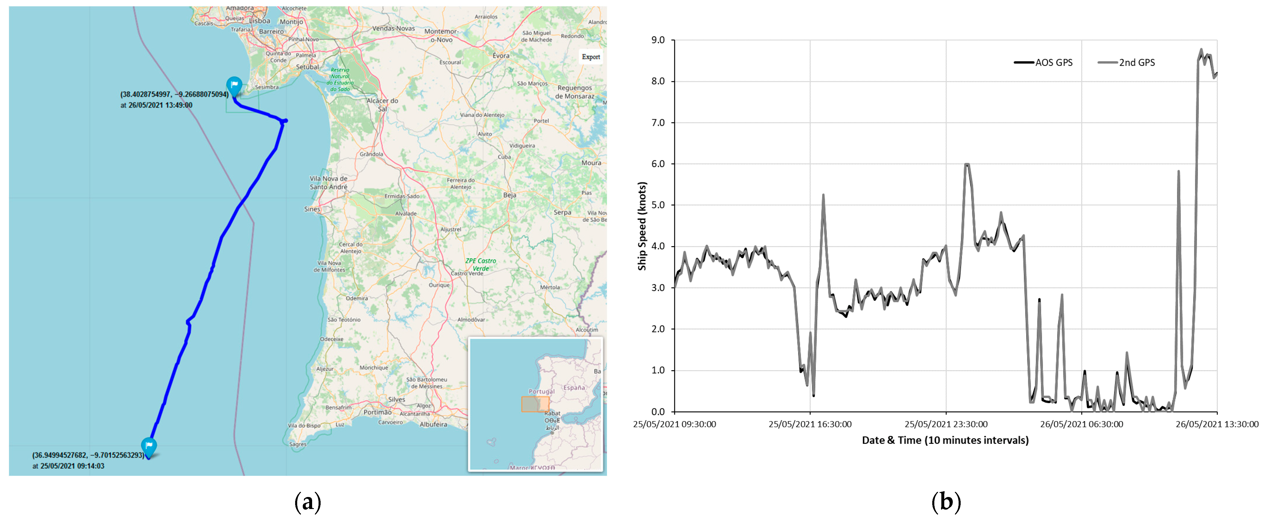
The meteorological parameters measured by the AWS include air temperature, relative humidity, barometric pressure, and wind speed and direction. The measurements cover the period from 09:20:00 on 25 May 2021 to 13:30:00 on 26 May 2021, corresponding to the selected route section of the research campaign, as depicted in
Figure 6a.
The AWS is configured to measure all the parameters with 10 min intervals, with the software outputting their averaged values, except for the barometric pressure and wind direction. The pressure data are sampled once at the end of each interval, while wind direction measurements, although taken as frequently as wind speed within the sampling interval, are categorized by the software into the respective “bins”. These bins correspond to the sixteen compass points, each spanning a range of 22.50°. This categorization occurs if the wind speed exceeds zero. At the end of the 10 min interval, the software identifies the predominant wind direction bin by determining which bin contains the highest number of values [
19].
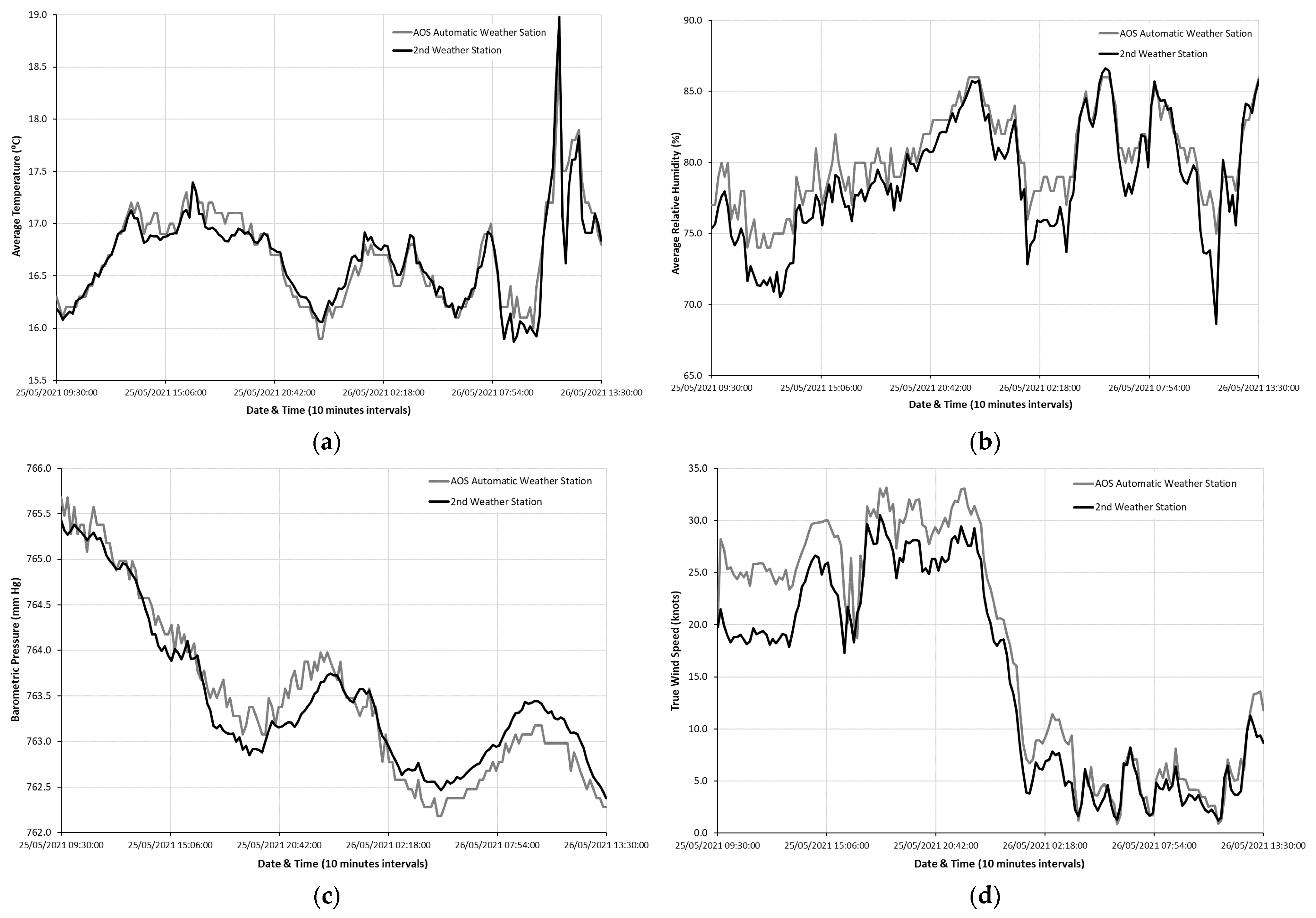
Figure 7a–d shows the plots of 10 min intervals data measured by the AOS automatic weather station and the second weather station for the following meteorologic parameters, respectively: average air temperature; average relative humidity; barometric pressure; and true wind speed.
The differences between both weather stations’ values for these parameters are given in
Table 7. The means and standard deviations values are acceptably low, which validates the readings. It should be mentioned that the true wind speed parameter has the highest mean difference and standard deviation, considering the range of its measured values. Upon observing
Figure 7d, the curves have a similar behaviour, and although differences between their values are larger in the first half of the plot, they converge approximately to the same values afterwards. This might have to do with the fact that both weather stations were placed around 5 m apart of each other and fixed into different structures of the deck above the bridge, which may differently affect locally the wind readings. Indeed, proper locations for wind sensors are particularly difficult to find as most sites for an anemometer to be placed will be affected by wind flow distortion over the superstructure [
11].
Figure 7 and
Table 7 show the performance of two sets of sensors. The data were collected to allow the assessment of the uncertainties than can be expected when using such types of equipment.
It is worth noting that the AWS’s anemometer automatically gives the apparent wind only, i.e., the wind relative to the anemometer’s arm (vessel framework). Thus, to obtain the true wind speed, the following was performed:
The anemometer’s arm was pointed to the bow of the ship upon its installation. This way, when the measured value of the apparent wind direction was 0° or 360°, the direction of the wind was known to be aligned with the ship’s bow.
The ship’s speed was estimated from the AOS GNSS data.
The true wind speed was obtained by subtracting the vessel’s SOG vector to the apparent wind speed vector given by the AWS anemometer, taking into account that the apparent wind direction was known, i.e., the angle of this vector relative to the ship’s bow.
4.2. Oceanographic Waves Parameters
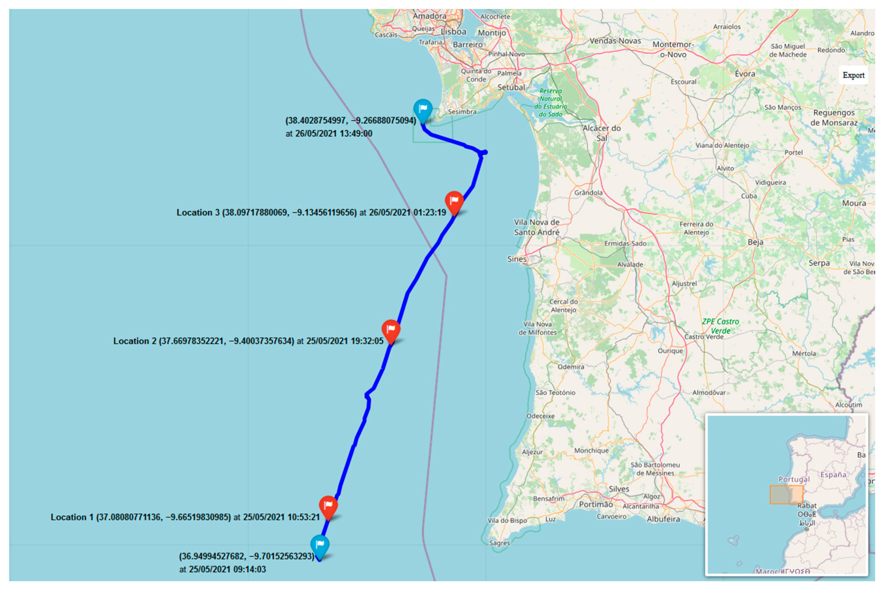
The oceanographic wave parameters and wave spectrum were estimated by the ocean wave estimator using genetic algorithms for a set of three selected locations along the RV’s route, as indicated in
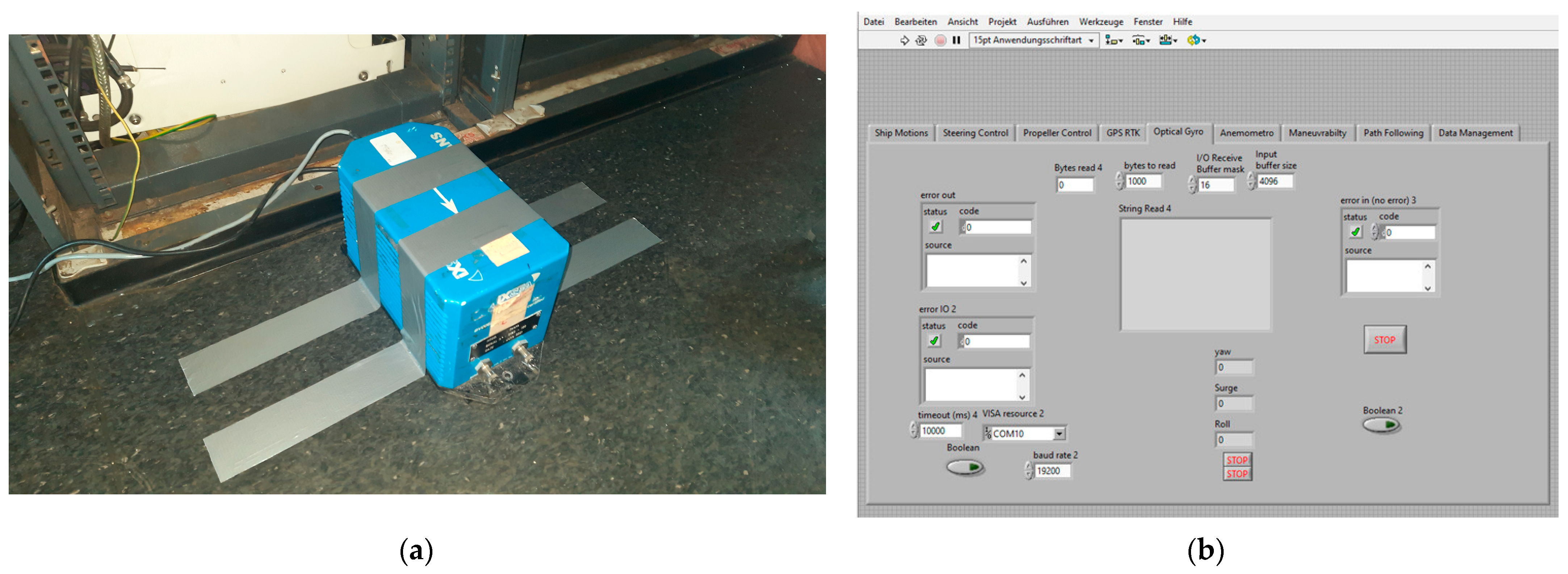
Figure 8. The estimations make use of the pre-estimated vessel’s RAO, which depends on the ship hull’s geometry, the ship’s SOG at the locations, and ship motions (heave, roll, and pitch) for 20 min of the IMU data in and near the locations, considering the correction due to the distance from where the IMU was placed in the bridge to the RV’s centre of gravity. The locations were chosen for the highest ship motions’ amplitudes. The estimation procedure is based on the method presented in [
16] and detailed in point 4 of
Section 3.2 of the current paper.
The estimator outputted the wave spectra, in polar form, and the following wave parameters: significant wave height (Hs in meters); peak wave period (Tp in seconds); peak intensification factor (γ); mean wave direction relative to the vessel’s stern (β in degrees); and wave spreading factor.
The estimations are validated against the forecasted data from the Copernicus’ ERA5 database containing hourly data on single levels from 1959 to the present [
32]. This ERA5 database is the fifth generation of the European Centre for Medium-Range Weather Forecasts (ECMWF) reanalysis for global climate and weather for the past decades, providing hourly estimates for a considerable set of atmospheric, ocean-wave, and land-surface parameters. The reanalysis product combines model data with worldwide observations into a globally complete and consistent dataset using the laws of physics, a principle named data assimilation, based on the method employed by numerical weather prediction centres. The dataset is a regridded subset of the complete ERA5 dataset on native resolution [
33]. The selected forecasted parameters for our case are the significant height of combined wind waves and swell (
Hs), peak wave period (
Tp), and true north mean wave direction (
β). A short description of these ERA5 parameters is given [
33]:
Significant height of combined wind waves and swell (Hs): This represents the mean height in meters of the highest third of surface ocean/sea waves produced by local winds and the related swell (this parameter takes both into account), meaning the vertical distance between the wave crest and wave trough. It is a parameter which is four times the square root of the integral over all directions and frequencies of the 2D wave spectrum.
Peak wave period (Tp): This represents the period in seconds of the most energetic oceans waves produced by local winds and the related swell (this parameter takes both into account), being calculated from the reciprocal of the frequency associated with the largest value (peak) of the frequency wave spectrum.
(True) mean wave direction (β): This represents the mean direction in degrees true of the ocean/sea surface waves generated by local winds and swell (this parameter takes both into account), consisting in the mean over all frequencies and directions of the 2D wave spectrum. The degrees true mean the direction relatively to the North Pole geographic location. It is the direction that waves are coming from. Thus, 0 and 90 degrees mean “coming from the North” and “coming from the East”, respectively.
These three parameters’ NetCDF data files were downloaded from the aforementioned database containing hourly data and using the reanalysis product. The chosen dates and times (UTC—universal time coordinated) for the data were based on the closest ones to each location in
Figure 8. It is important to refer that the time zone at the locations in May is UTC + 1. So, for example, location 1 AOS GNSS and IMU data are from 10:53:21 AM UTC + 1, which led to selecting Copernicus ERA5 data from 10:00 AM UTC, i.e., meaning 11:00 AM in UTC + 1 time zone of location 1.
The NetCDF files of these parameters have a latitude-longitude grid of 0.5 × 0.5 degrees for the reanalysis. Afterwards, climate data operators (CDOs) commands were used in a Windows® Cygwin64© terminal for regridding to 0.01 × 0.01 degrees.
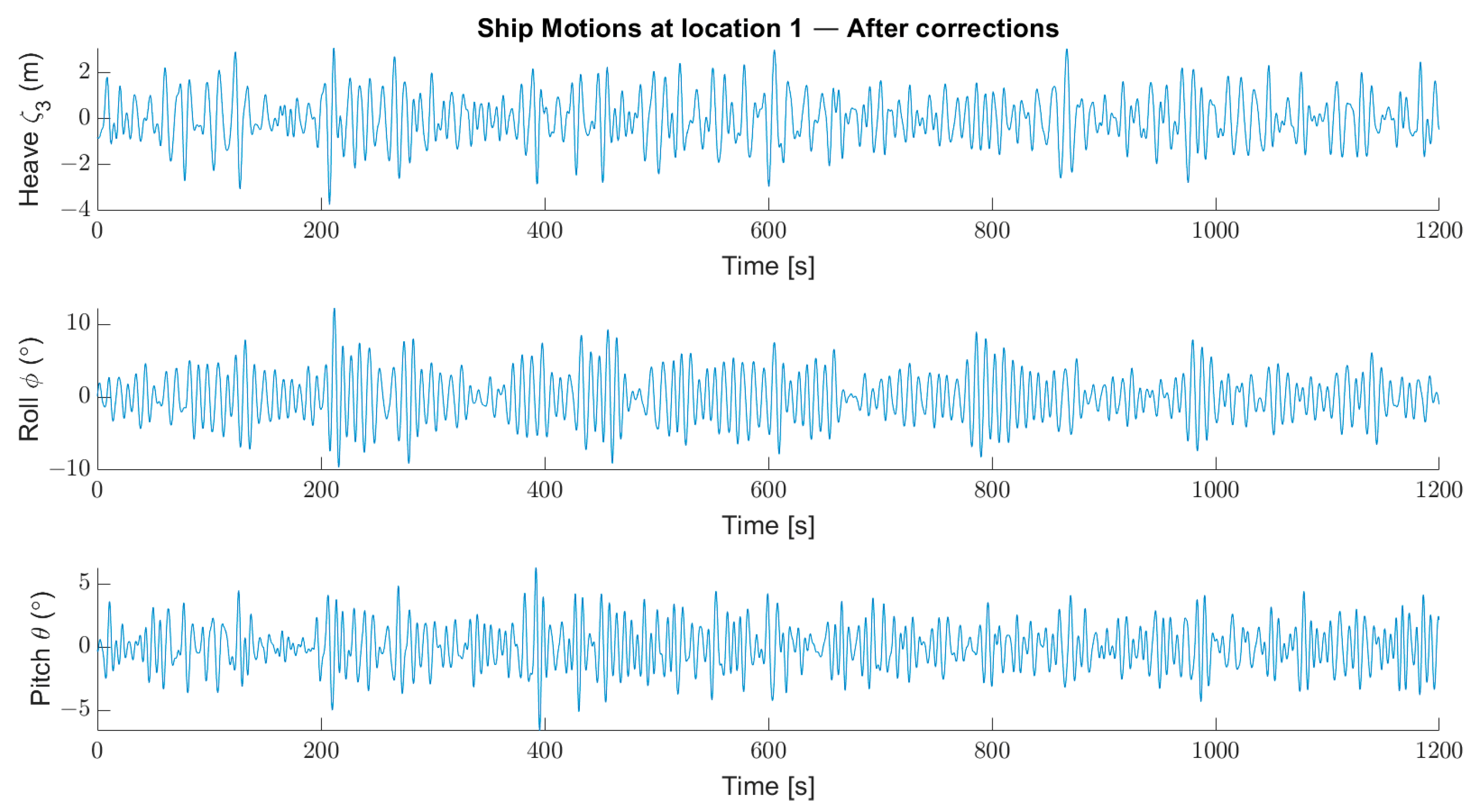
Figure 9 shows the ship motions, heave, roll, and pitch for a period of 20 min IMU readings when the RV was passing through location 1. These ship motions were based on the IMU’s data and corrected by considering the distance from the IMU to the vessel’s centre of gravity. This approach is also used for ship motions at locations 2 and 3.
The recorded ship motions are high. The highest roll values are over 10 degrees at locations 1 and 2, and the heave motions reach values higher than 3 m at location 1, all due to the bad weather experienced at that time. The length of the time series is 20 min, which can be considered a constant sea state.
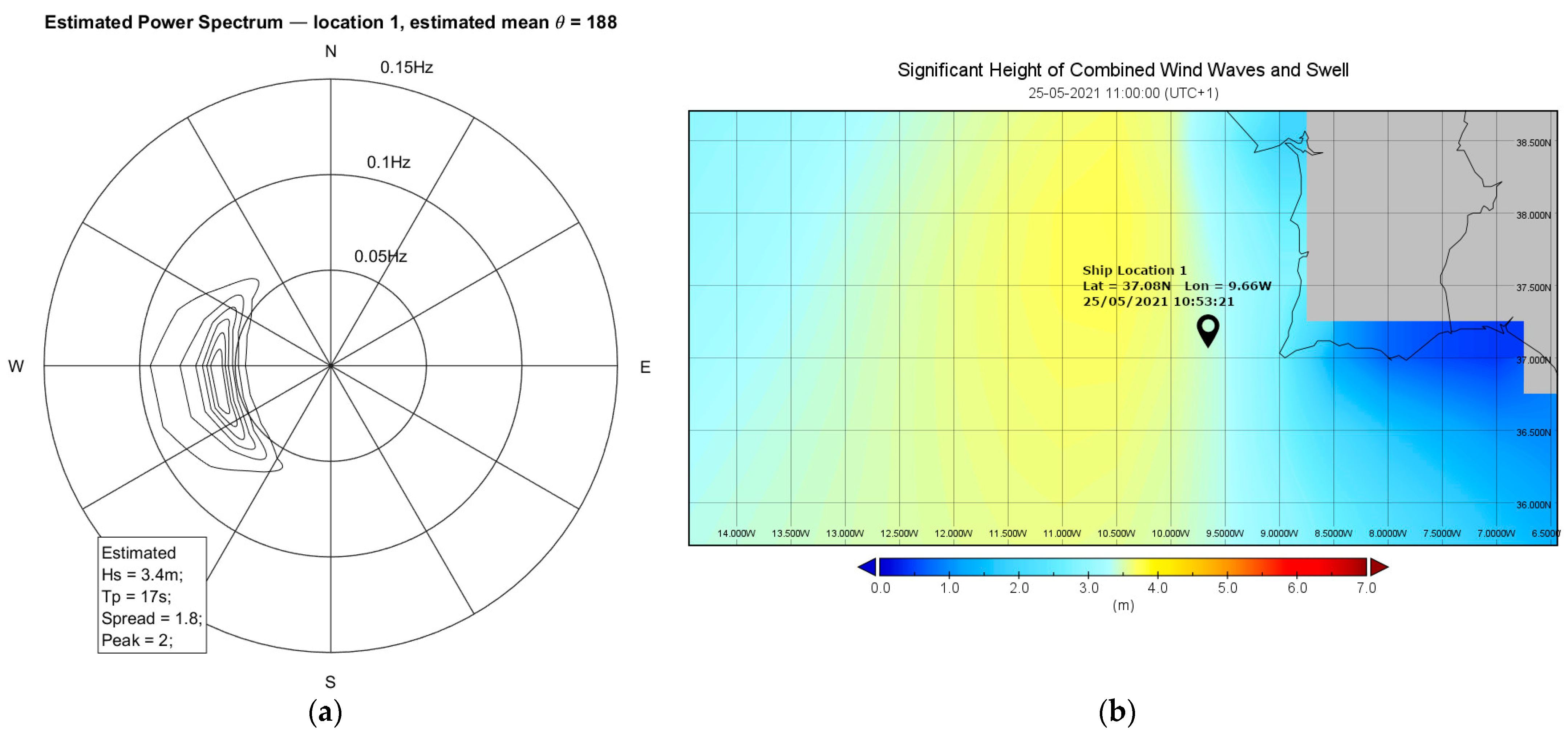
Figure 10a presents the estimated wave spectrum in polar form for location 1 considering the 20 min corrected ship motions, whereas
Figure 10b shows the forecasted significant height of the combined wind waves and swell at the same location obtained from data from the Copernicus database and using the Panoply netCDF, HDF and GRIB Data Viewer running on Windows
® platform [
34]. This approach is also used for data of locations 2 and 3.
At location 1 and looking to
Figure 10a, the estimated wave spectrum has a significant wave height
Hs = 3.4 m, wave period
Tp = 16.8 s, and mean wave direction
θ = 188° (with respect to the ship stern). The estimated wave spectra have good agreement for the significant wave height as they are approximately the same as the forecasted ones (see
Figure 10b), as can be seen in
Table 8. But, in the estimation of the wave period and mean wave direction, some errors arise since the minimization function depends on the energy content below the power curve. The directional spectra not only consider the three parameters discussed before but also depend on the spreading function and peak enhancement factor
γ. The estimated wave direction is 188° which indicates the ship encountered head waves, thus meaning predominant heave and pitch ship motions as can be observed in the corrected IMU measurements in
Figure 9.
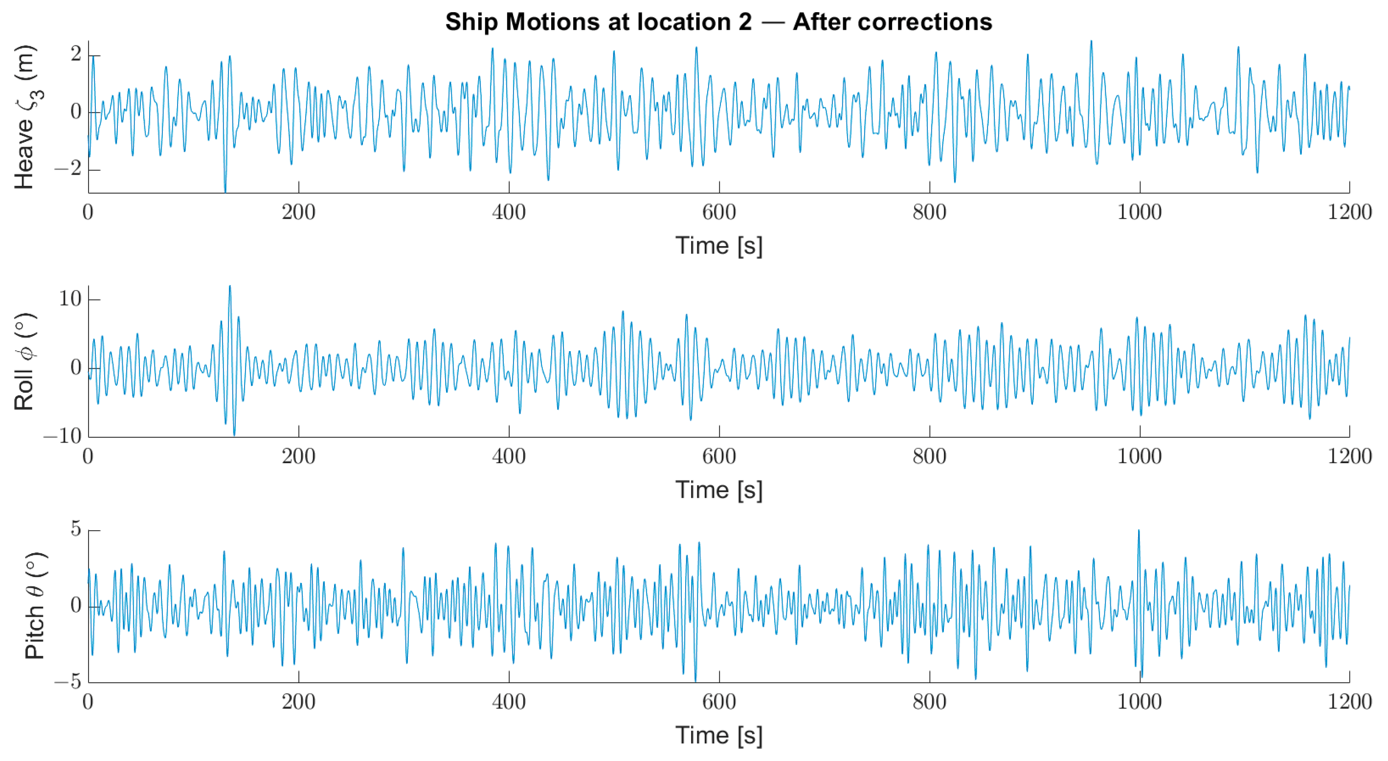
At location 2, the estimated mean wave direction is close to 180°, which indicates the ship encountered head waves, thus meaning predominant heave and pitch ship motions occurred, as can be observed in the corrected IMU measurements in
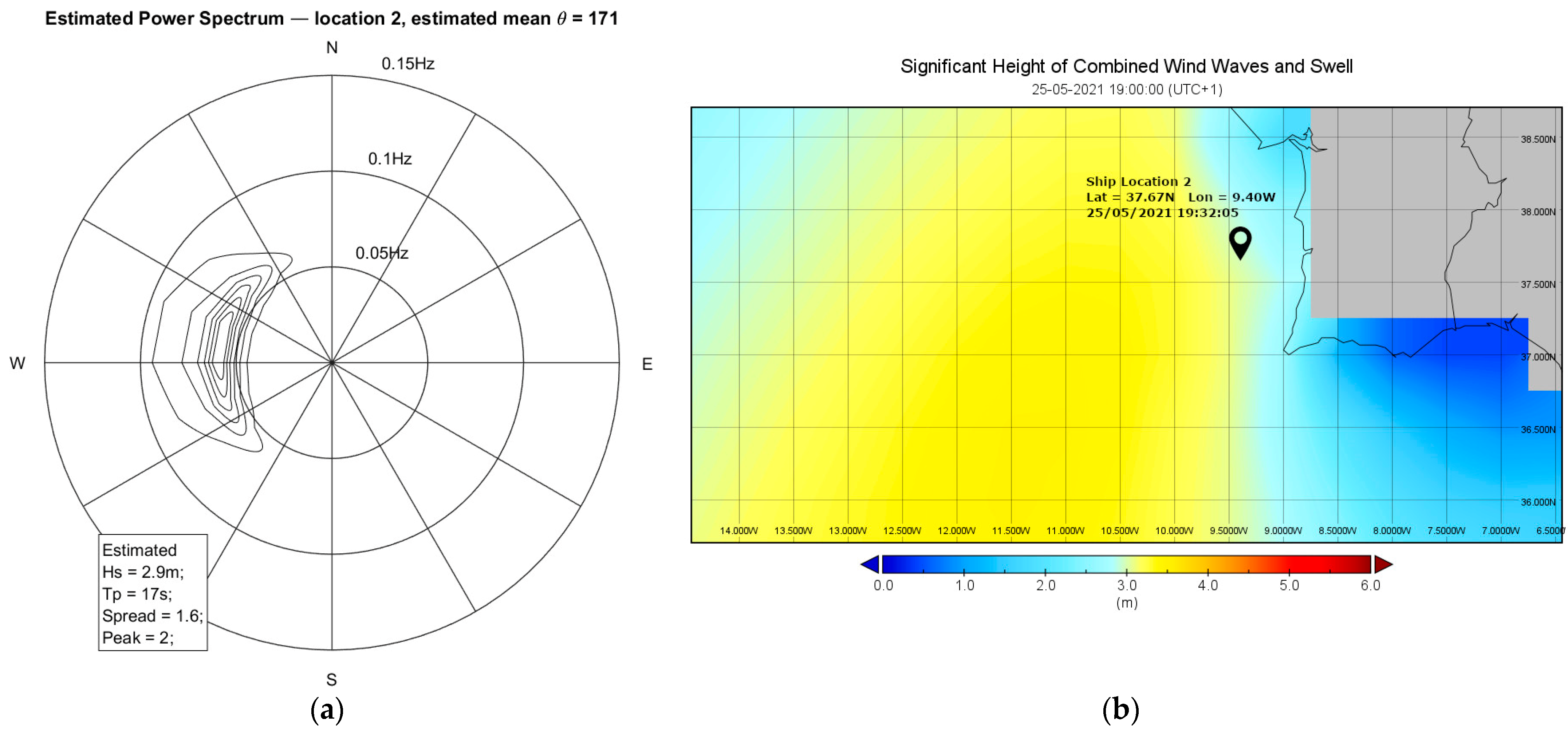
Figure 11. Looking to
Figure 12a, the estimated wave spectrum has a significant wave height
Hs = 2.9 m, wave period
Tp = 17 s, and mean wave direction
θ = 171° (with respect to the ship stern). The estimated wave spectra have good agreement for the significant wave height when compared to the forecasted ones (see
Figure 12b), but in the estimation of the wave period, the errors are high (see
Table 8), since the minimization function depends on the energy content below the power curve.
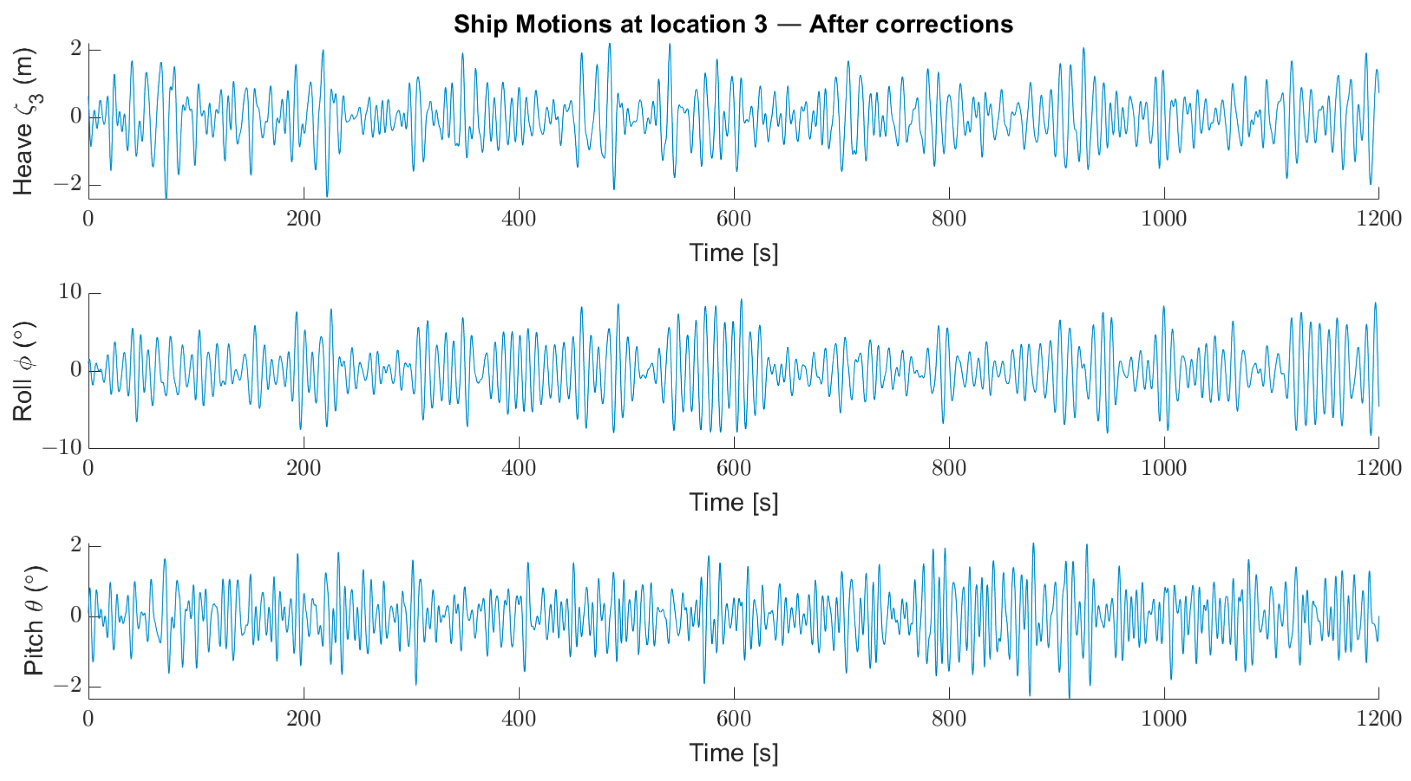
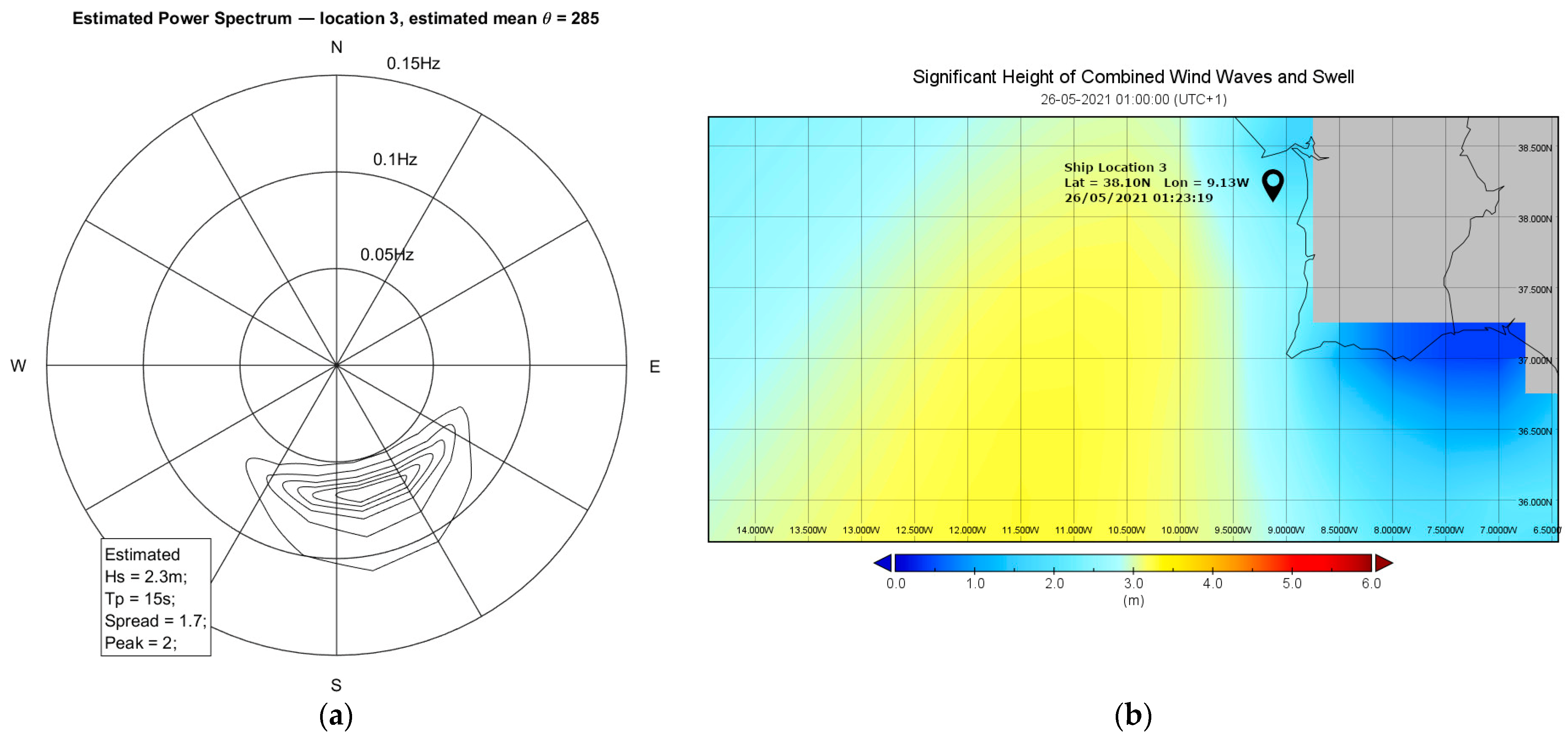
At location 3, the estimated mean wave direction is 285°, which indicates the ship encountered beam waves, thus meaning the roll motions are higher than the heave and pitch motions, as can be observed in the corrected IMU measurements in
Figure 13. Looking at
Figure 14a, the estimated wave spectrum has a significant wave height
Hs = 2.3 m,
Tp = 15 s and mean wave direction
θ = 285° (with respect to the ship stern). The estimated wave spectra have good agreement for the significant wave height and wave period (see
Table 8).
Table 8 presents, for all three locations, the estimated results from the wave spectrum estimator and forecasted values from the Copernicus database for several wave parameters, namely, significant wave height, peak wave period, peak intensification factor, mean wave direction, and wave spreading factor. The wave estimation algorithm considers combined wind waves and swell.
The method that estimates the wave spectrum, which basically estimates the spectrum energy, depends on the assumption of a parametric representation of the wave spectrum. In this study, the model used is the well-known JONSWAP spectrum. This model has five parameters, namely, the significant wave height, wave period, wave direction, spread function, and peak factor. The errors related to the estimation of one of those parameters are subjected to the estimation of the others. Thus, in our estimations, the errors obtained for the significant wave height are low, which affects the estimations in the wave period.
The wave spectrum estimator has, as a reference frame, the ship axis coordinates, where the positive x-direction is equivalent to head waves (180°). The Copernicus database reference frame axis is based on true north (north is equivalent to 0°).
The errors given in
Table 8 for significant wave height and wave period are calculated by
The error in wave direction is the difference between the forecasted and estimated data (
θ in
Figure 10a,
Figure 12a and
Figure 14a). From
Table 8, it is possible to see errors around 30° for locations 1 and 2. These errors are acceptable considering that the estimation algorithm and the vessel’s RAO have a 20 degrees grid. The following is an example of the error calculation for the wave direction:
Location 1: 188° relatively to the vessel’s stern, as seen in
Figure 10a (equivalent to 172° due to ship symmetry), and 14° true heading (from IMU). So, the wave direction is 180° − 172° = 8° starboard relatively to the bow, and we must add it to the 14° true heading, giving 14° − 8° = 6° true wave direction. Therefore, the error is (|Forecasted − Estimated|) = |336° − (360° + 6°)| = 30°.
5. Discussion
The data and results obtained from the full-scale trial have shown that the presented AOS prototype can be a feasible approach to collect and integrate meteorological and oceanographic data obtained onboard a VOO.
The meteorological parameters measured by the AWS over 10 min archive intervals were validated against the readings of a second weather station. The differences between the mean values of both stations were 0.11 °C, 1.63%, 0.22 mmHg, and 2.96 knots for the average temperature, average relative humidity, barometric pressure, and true wind speed, respectively. The standard deviations were of the same order of magnitude. These values are reasonably low, thus validating the readings.
Oceanographic wave parameters and wave spectra were estimated by an ocean wave estimator, using genetic algorithms for optimization and a short computational time, for three selected locations along the RV’s route. The estimator outputted the wave spectra, in polar form, and wave parameters such as the significant wave height, peak wave period, peak intensification factor, mean wave direction, and wave spreading factor. Estimations relied, at each location, on the ship’s SOG and on 20 min of IMU ship motions data (heave, roll, and pitch), corrected due to the distance of the IMU to the RV’s centre of gravity. These estimations were validated with forecasted wave data from the Copernicus’ ERA5 database.
The results of the wave estimator for the significant wave height have good agreement with the forecasted ones from the Copernicus database as the errors are below 3%. The errors for the wave period are around 16–28%, which is reasonable for one of the locations, but in the other two, the errors are higher since the minimization function depends on the energy content below the power curve. Moreover, the errors associated with the estimation of one of these parameters are subjected to the estimation of the others. Consequently, the errors obtained in the estimations for the significant wave height are low, which affects the estimations in the wave period. Concerning the mean waves directions, the errors are between 30° and 45°, but for two of the locations, the errors are acceptable, given that the estimation algorithm and the vessel’s RAO have a 20 degrees grid. Additionally, the estimated mean waves directions are in accordance with the effects of the waves in the ship motions (heave, pitch, roll) observed in the corrected measurements of the IMU. An improvement would involve developing an algorithm to conduct online validations with the NOAA database.
6. Conclusions
The current paper describes an AOS prototype consisting of an AWS, IMU, and a GNSS unit installed onboard a Portuguese RV and shows the respective underway measurements obtained during a full-scale trial off the coast of Portugal along with wave parameters estimated with an ocean wave estimator.
The presented AOS prototype demonstrated its potential as a feasible approach for collecting quality environmental data, integrating meteorological and oceanographic data collected onboard VOO. The system has been designed to be installed in fishing vessels that will operate as VOO and as a distributed network of ocean data collection.
While data such as wind speed and wave height can be obtained from weather satellites, the information collected by VOO plays a crucial role in not only confirming the accuracy of remotely acquired data but also in validating and enhancing the results of computer numerical models [
35], such as the ones used in larger and mesoscale scientific climate studies, and also in smaller coastal scale projects, such as the ones related to coastal ocean engineering works (e.g., ports construction, renewable offshore winds, and waves energy).
The AWS and the anemometer are self-contained pieces of equipment powered by a lithium battery and a solar panel, with large autonomy lasting around two years with the same battery [
18]. Additionally, the communication between the AWS and its indoor console connected to the ODC is wireless, simplifying the installation and maintenance, given that there is no need for cabling.
The wave estimator using an IMU can be a cost-effective alternative solution to wave radars, as the IMUs can be cheaper and be installed indoors in the ship’s bridge away from the harsh maritime environment, reducing the need for difficult installations of a radar on top of the mast or on the ship’s bow plus long cablings, reducing maintenance time and costs and acquisition costs, given that wave radars are quite expensive. Improvements of the wave estimator algorithm for enhanced accuracy can be possible with more testing of the AOS after its installation in fishing vessels working as VOO for ocean data collection.


 ,
, 


