Communication

Smart Structures Innovations Using Robust Control Methods

by
Amalia Moutsopoulou
1,*,
Georgios E. Stavroulakis
2,
Markos Petousis
1,
Nectarios Vidakis
1 and
Anastasios Pouliezos
2
1
Department of Mechanical Engineering, Hellenic Mediterranean University, Estavromenos, 71410 Heraklion, Greece
2
Department of Production Engineering and Management, Technical University of Crete, Kounoupidianna, 73100 Chania, Greece
*
Author to whom correspondence should be addressed.
Appl. Mech. 2023, 4(3), 856-869; https://doi.org/10.3390/applmech4030044
Submission received: 10 June 2023 / Revised: 9 July 2023 / Accepted: 18 July 2023 / Published: 19 July 2023

Abstract

:
This study’s goal is to utilize robust control theory to effectively mitigate structural oscillations in smart structures. While modeling the structures, two-dimensional finite elements are used to account for system uncertainty. Advanced control methods are used to completely reduce vibration. Complete vibration suppression is achieved using advanced control techniques. In comparison to traditional control approaches, Hinfinity techniques offer the benefit of being easily adaptable to issues with multivariate systems. It is challenging to simultaneously optimize robust performance and robust stabilization. One technique that approaches the goal of achieving robust performance in mitigating structural oscillations in smart structures is H-infinity control. H-infinity control empowers control designers by enabling them to utilize traditional loop-shaping techniques on the multi-variable frequency response. This approach enhances the robustness of the control system, allowing it to better handle uncertainties and disturbances while achieving desired performance objectives. By leveraging H-infinity control, control designers can effectively shape the system’s frequency response to enhance stability, tracking performance, disturbance rejection, and overall robustness.

1. Introduction

Smart structures have garnered significant attention in recent years due to their immense potential and wide-ranging applications. A smart structure is defined as one that intelligently perceives mechanical disturbances and automatically reacts to them by reducing oscillations [1,2,3]. The field of smart structures has seen a big increase in recent years [3,4,5,6]. In this work, an intelligent structure that has integrated actuators and sensors that are capable of damping the oscillations is presented [7,8,9,10]. Dynamic loads such as wind forces are applied and finite element analysis is performed [1,6,11,12]. Advanced testing techniques such as robust control theory are used. It is then applied to engineering applications that are made with smart materials such as piezoelectric material. In these constructions, both sensors and actuators are integrated; the actuators achieve the suppression of the oscillation [9,10,11]. Many researchers have mainly dealt with the modeling of these constructions but also with the application of advanced control techniques [2,12,13,14,15,16]. Modeling and control techniques are often used for the analysis of optimization of the materials response [17,18,19,20,21]. In addition, many researchers have engaged in research on composite concrete structures in the frequency domain and have presented very good results in solving optimization problems [22,23] in this field; they are many practical applications from important researchers [24,25].
Our paper provides the innovation in the piezoelectric intelligent structures with robust control theory. We achieve complete vibration suppression even for uncertainty modeling of the smart structure. This work has provided many innovations in the suppression of oscillations with the application of smart materials:
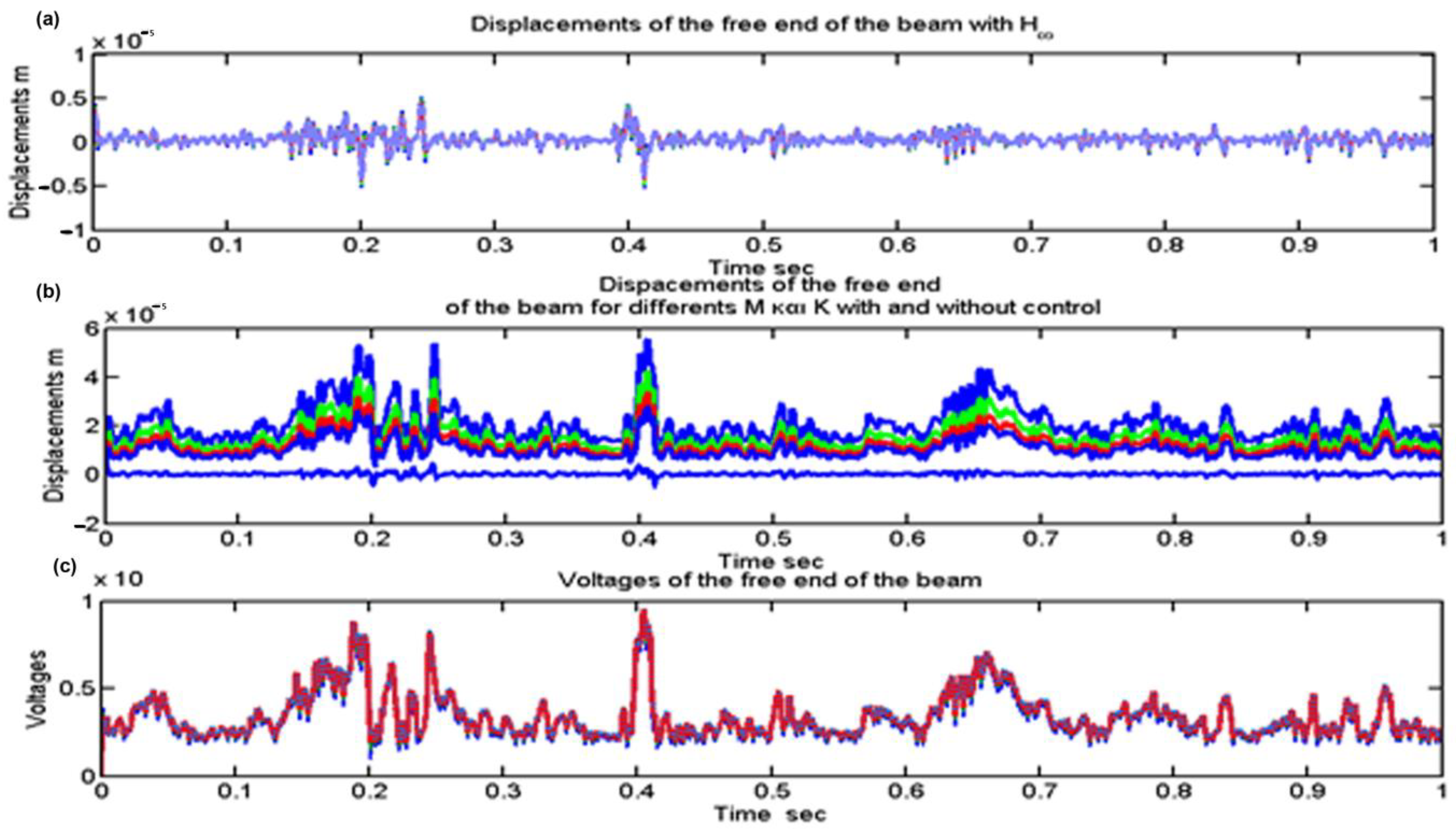
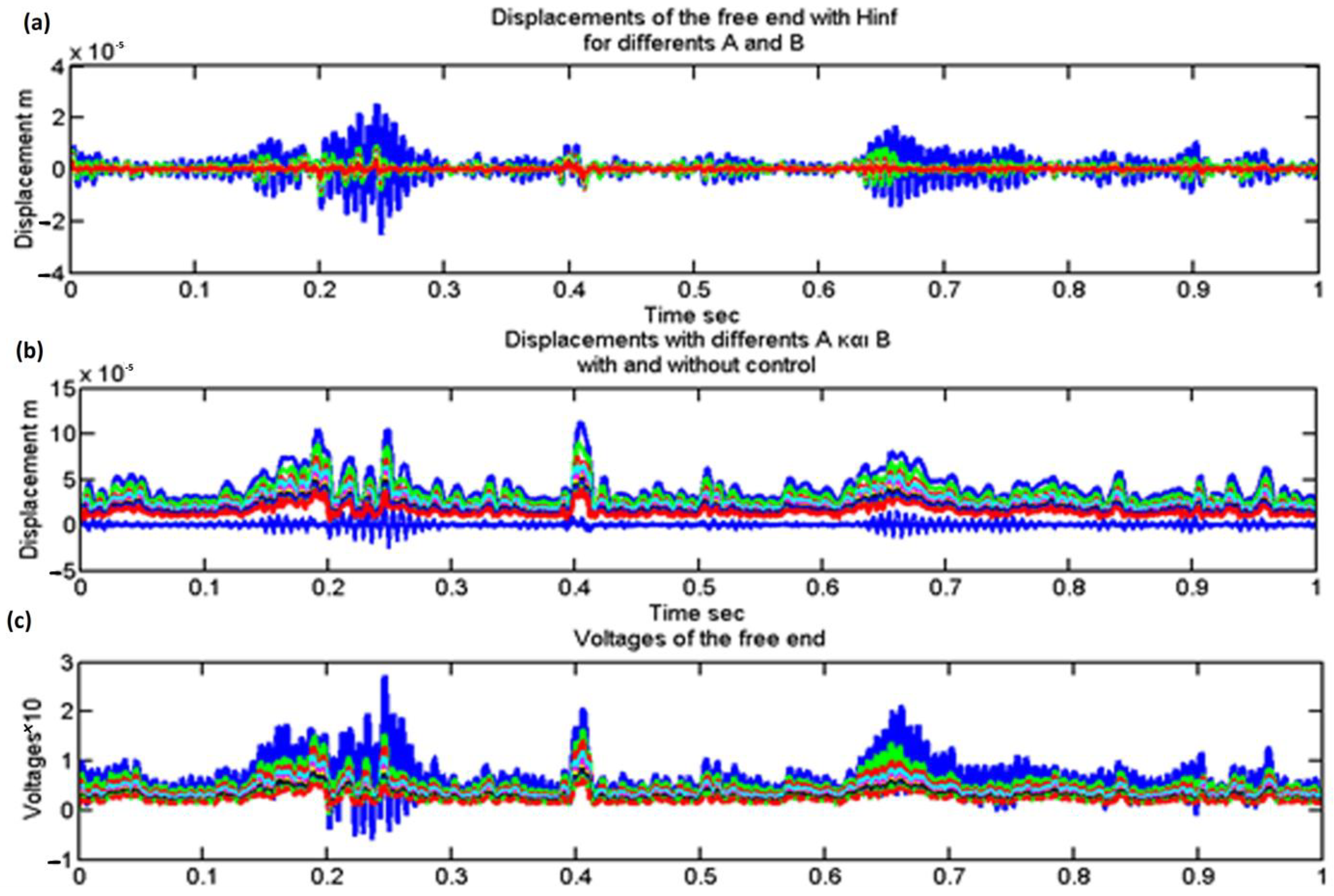
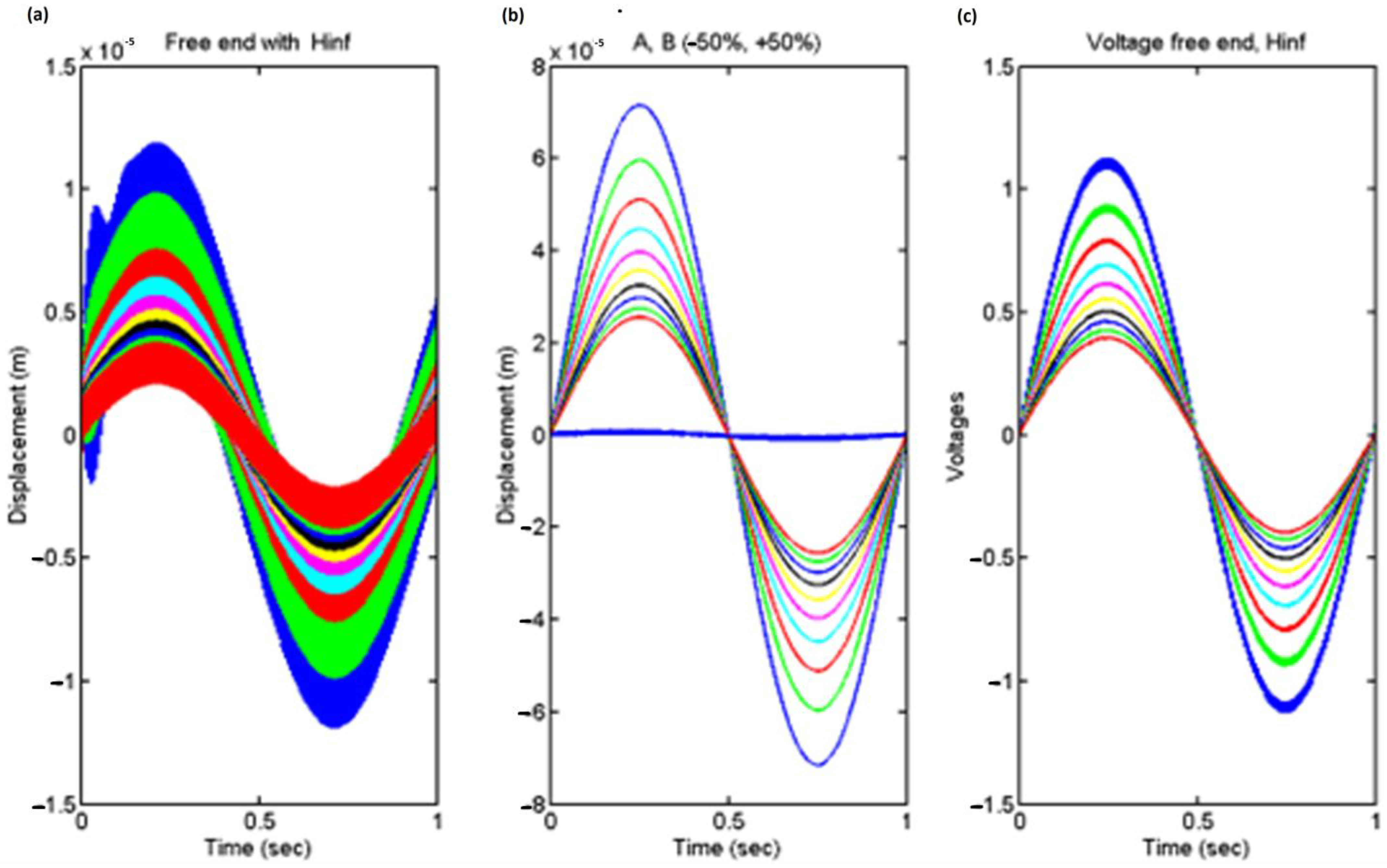
  • With the help of advanced control techniques such as the Hinfinity Control, the reduction of oscillations is achieved even for changes in the mass and stiffness of the original model that is presented for modeling uncertainties.
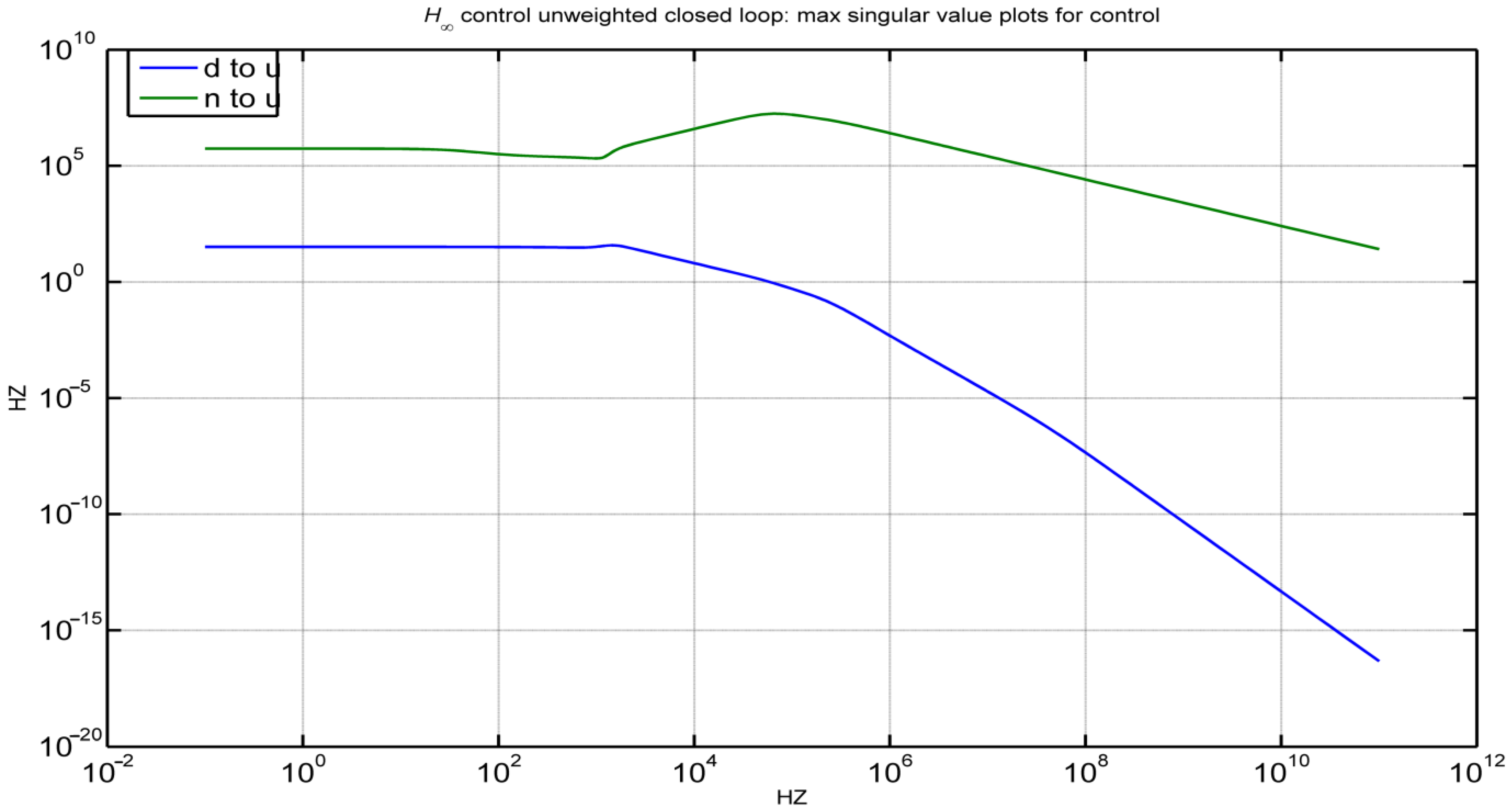
  • By demonstrating the use of Hinfinity control in both the state space and frequency domain, the study explores the benefits of robust control in intelligent structures. It takes into consideration a dynamic model for intelligent constructions subject to excitations induced by the wind.
  • The Hinfinity robust controller solves the dynamical system uncertainties and the partial data measurements to make the design possible. The effectiveness of the suggested strategies to reduce vibrations in piezoelectric smart structures is demonstrated by numerical simulations. The strategy guarantees a thorough and unified process for creating and verifying reliable control systems.
  • The Hinfinity robust controller aids in the creation of intelligent structures by taking into account dynamical system uncertainties and partial data.
  • Notably, advances in intelligent structures with advanced control methods have been well demonstrated.

2. Materials and Methods

The system’s dynamical description is provided by,
M q ¨ ( t ) + D q ˙ ( t ) + K   q ( t ) = f m ( t ) + f e ( t )
The independent variable q(t) represents the collective behavior of the system, including transversal deflections wi and rotations ψi. It is influenced by several factors, including the external loading vector fm, which represents the applied external forces, the generalized control force vector fe, which arises from electromechanical coupling effects, the generalized stiffness matrix K, which characterizes the structural stiffness, the generalized mass matrix M, which describes the mass distribution, and the viscous damping matrix D, which accounts for energy dissipation due to damping effects. These factors collectively contribute to the dynamic response and behavior of the system, i.e.,
q ( t ) = w 1 ψ 1 w n ψ n
The parameter n in the analysis refers to the number of nodes present in the finite elements under consideration. Both the w and fm vectors point upward [10,15,16].
To convert to a state-space control representation, we can perform the transformation (as typically carried out) by defining the following:
x ( t ) = q ( t ) q ˙ ( t )
Additionally, we can specify the generalized con d as, and the voltages u applied to the actuators. This allows us to represent fe(t) as Bu(t), where the control force vector fe(t) is a function of the piezoelectric force per unit displacement; denote B captures the relationship between the piezoelectric force and the applied voltages. Additionally, we define the disturbance vector as d(t) = fm(t). Nonetheless,
x ˙ ( t ) = 0 2 n × 2 n I 2 n × 2 n M 1 K M 1 D x ( t ) + 0 2 n × n M 1 f e * u ( t ) + 0 2 n × 2 n M 1 d ( t ) = A x t + Β u t + Gd t = Ax t + B   G = Ax t + B ~ u ~ ( t )
By considering the output equation, which involves only measuring the displacements, denoted as [10], we can enhance the representation further.
y(t) = [x1(t), x3(t) … xn−1(t)]T = Cx(t)
In this particular formulation, the control input vector u is represented by an n × 1 matrix, where n is the number of nodes in the system. However, the control input vector can be smaller than n. On the other hand, the disturbance vector d has a size of 2n × 1. The measurement units used in this formulation are meters (m) for displacement, radians (rad) for rotations, seconds (s) for time, and Newtons (N) for force. These units are utilized to quantify the physical quantities and dimensions involved in the system’s analysis and control.
The primary objective of the control task is to maintain the beam in a state of equilibrium. This means ensuring that the displacements and rotations of the beam are kept at zero, indicating a stable and balanced state [26,27]. The control inputs are utilized to counteract the effects of external disturbances, noise, and potential inaccuracies in the model, thereby actively adjusting the system to maintain the desired equilibrium state. By effectively compensating for these disturbances and model uncertainties, the control system aims to achieve and sustain the desired zero displacements and rotations, ensuring stability and optimal performance of the beam [27,28].

3. Robustness Analysis

The following three stages will be performed in a robustness analysis:
  • The range of uncertainty that a mathematical model expresses.
  • Robust stability (RS): For each plant included in the uncertainty set, verify the system’s stability.
  • Robust performance (RP) refers to the degree of stability exhibited by a system. In the context of investigating robust performance, the goal is to determine whether any of the plants included in the uncertainty set meet the specified performance criteria. This involves analyzing the system’s behavior under various uncertain scenarios and assessing if the performance requirements are satisfied for each plant within the uncertainty set [24,25,26].
The robustness investigation will be performed using the connections shown in Figure 1.
Here, K is the estimated Hinfinity controller, and P is the nominal plant with the uncertainty modeling included. Uncertainty included in Δ satisfies ║Δ║∞ ≤ 1 [26,27].
Since Ks is the known controller, Figure 1 can be simplified to Figure 2.
This arrangement makes it clear that,
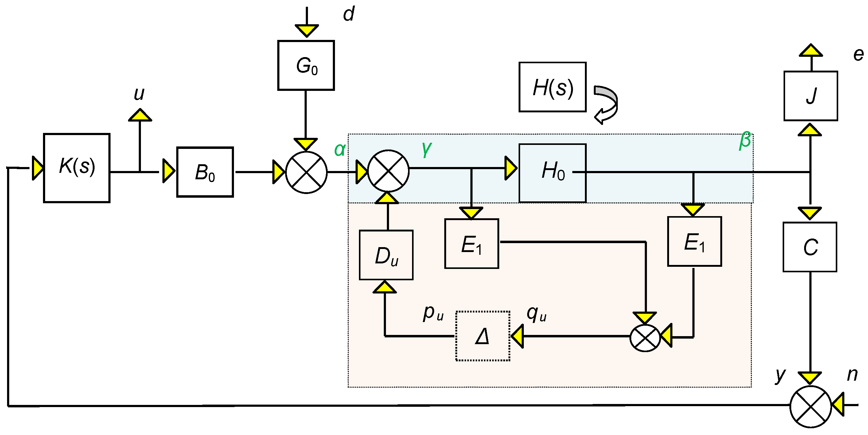
  • The system (M, Δ) is considered to be robustly stable if it satisfies two conditions:
    • The nominal system M is stable, meaning that it does not exhibit any instability or unbounded responses in the absence of uncertainties.
    • The system remains stable under all possible variations or uncertainties represented by the structured uncertainty set Δ. In other words, the system maintains stability even when the uncertain parameters or inputs vary within the prescribed uncertainty bounds [27,28].
By satisfying these two conditions, the system (M, Δ) is deemed to be robustly stable, demonstrating stability and resilience in the face of uncertainties:
sup ω R μ Δ M 11 ( j ω ) < 1
where,
1 μ B ( M ) = i n f Δ B Δ , d e t ( I M Δ ) = 0 σ - ( Δ )
The structured singular value of M, denoted as μ(M), is a measure of robust stability. It quantifies the largest multiplicative uncertainty that a given system M can tolerate within the structured uncertainty set BΔ while remaining stable. Hence, the robust stability of the system (M, Δ) is achieved when the structured singular value of M, μ(M), exceeds one.
  • The system (M, Δ) is said to exhibit robust performance if it satisfies the specified performance criteria despite the presence of uncertainties represented by the structured uncertainty set Δ. Robust performance implies that the system can maintain desired performance levels, such as stability, tracking accuracy, disturbance rejection, or other performance metrics, even in the presence of uncertainties. Achieving robust performance involves designing control strategies or mechanisms that can effectively handle and mitigate the effects of uncertainties within the specified performance bounds,
s u p ω R μ Δ α M ( j ω ) < 1
where,
Δ α = Δ p 0 0 Δ
The uncertainty set Δp has a similar structure to Δ but with dimensions corresponding to (w, z) [9,27,28]. To proceed, let us consider uncertainties in the form of variations or perturbations in the M (mass), D (damping), and K (stiffness) matrices,
M = M0(I + mpδM)
D = D0(I + dpδD)
K = K0(I + kpδK)
with,
Δ δ M δ D δ K < 1
By allowing a percentage deviation from the nominal values, we accommodate variations in the M (mass), D (damping), and K (stiffness) matrices. With these definitions, Equation (1) can be expressed as follows:
M 0 ( I + m p δ M ) q ¨ t   + D 0 ( I + d p δ D ) q ˙ t   + K 0 ( I + k p δ K ) q t   = f m ( t ) + f e ( t ) M 0 q ¨ t   + D 0 q ˙ t   + K 0 q ( t ) = [ M 0 m p δ M q ¨ t   + D 0 d p δ D q ˙ t   + K 0 k p δ K q t ]   + f m ( t ) + f e ( t ) M 0 q ¨ t   + D 0 q ˙ t   + K 0 q ( t ) = D ~ q u t   + f m ( t ) + f e ( t )
where,
q u ( t ) q ¨ ( t ) q ˙ ( t ) q ( t ) , D ~ =   M 0 m p D 0 d p K 0 k p I 2 n × 2 n δ M I 2 n × 2 n δ D I 2 n × 2 n δ K
Writing (5) in state space form, gives,
x ˙ ( t ) = 0 2 n × 2 n I 2 n × 2 n M 1 K M 1 D x ( t ) + 0 2 n × n M 1 f e * u ( t ) + 0 2 n × 2 n M 1 d ( t ) + 0 2 n × 6 n M 1 D ~ q u ( t ) = A x t + Β u t + Gd t + G u q u ( t )
In this approach, we account for the uncertainty in the original matrices by treating it as an additional factor of uncertainty. To represent our system in the frequency domain as depicted in Figure 2, we consider the configuration shown in Figure 3.
The matrices E1 and E2 are exploited to derive,
q u ( t ) q ¨ ( t ) q ˙ ( t ) q ( t )
Since,
γ = q ¨ ( t ) q ˙ ( t )   and   β = q ¨ ( t ) q ˙ ( t ) = q ˙ ( t ) q ( t )
Possible selections for E1 and E2 depend on the specific situation and criteria of the system,
E 1 = I 0 0 I 0 0 , E 2 = 0 0 0 0 0 I
The idea is to find an M such that,
q u e u = M p u d n , M = M 11 M 12 M 13 M 21 M 22 M 23 M 31 M 32 M 33 = M p u q u M d q u M n q u M p u e M de M ne M p u u M du M nu
Alternatively, in the notation depicted in Figure 3,
q u w = M p u z
Now Mde, Mdu, Mne, and Mnu, are known:
M d e M n e M d u M n u = J ( I H B K C ) 1 H G J ( I H B K C ) 1 H B K ( I K C H B ) 1 K C H G ( I K C H B ) 1 K
To proceed with the methodology known as “pulling out the Δ’s”, we will break the loop at points pu and qu, utilizing the auxiliary signals α, β, and γ. This approach will allow us to derive the transfer function. M d q u (from d to qu):
qu = E2β + Ε1γ = (E2H + Ε1
γ = Gd + Bu = Gd + BKCHγ ⇒ γ = (Ι-BKCH)−1 Gd
Hence,
M p u q u = ( E 2 H + E 1 ) ( Ι-BKCH ) 1 G
Now, M p u q u , M p u e , M p u u , are similar to Mde, Mde, and Mdu with G switched by Du, i.e.,
M p u q u = ( E 2 H + E 1 ) ( Ι-BKCH ) 1 D u
M p u e = J ( I H B K C ) 1   H D u
M p u u = ( I K C H B ) 1 K C H D u
Finally, to find M n q u ,
qu = E2β + Ε1γ = (E2H + Ε1
γ = Bu = BK(n + y) = BKn + BKCHγ ⇒ γ = (Ι-BKCH)−1 ΒΚn
Hence,
M n q u = ( E 2 H + E 1 ) ( Ι-BKCH ) 1 B K
Collecting all the above yields M:
M = ( E 2 H + E 1 ) ( I B K C H ) 1 D u ( E 2 H + E 1 ) ( I B K C H ) 1 G ( E 2 H + E 1 ) ( I B K C H ) 1 B K J ( I H B K C ) 1 H D u J ( I H B K C ) 1 H G J ( I H B K C ) 1 H B K ( I K C H B ) 1 K C H D u ( I K C H B ) 1 K C H G ( I K C H B ) 1 K

4. Results

Figure 4a,b shows a cantilever smart beam with piezoelectric actuators and a sensor. It used the Euler-Bernoulli formulation. The beam’s specifications are given in Table 1. The beam has dimensions L × W × H, representing its length, width, and height. The piezoelectric sensors have a width of bS, while the piezoelectric actuators have a thickness of bA.
First, a wind force acting on the side of the smart beam is taken. The function d(t) = fm(t), in Figure 5, is determined from the record of wind speed using the relation
f m ( t ) = 1 2 ρ C u V 2 ( t )
where ρ = density, V(t) = velocity, and Cu = 1.5 (orthogonal cross-section)
The mechanical force was calculated using actual wind speed measurements made in Estavromenos, Heraklion Crete. Furthermore, measurements at the system’s response sites were exposed to random noise with a probability of 1% in all simulations. As a result of the system nodal points’ minor displacements, the noise amplitude is considered to be minimal, on the order of 5 × 10⁻⁵ of the initial pricing. However, each node of the beam introduces a different proportion of the signal, with the first node’s percentage being lower due to the clamping of the beam’s endpoint.
Figure 6 depicts the translation of the free end of the beam in the state space domain for closed and open loops with varied mass and stiffness matrices. Figure 6b (middle graphic) depicts the displacement of the cantilever beam’s free end for various stiffness and mass matrices (i.e., by changing mp, kp in the relation M = M0(I + mp δM), K = K0(I + kpδK). This displacement is shown in Equation (6) as a function of the stiffness and mass matrices. The blue diagram represents mp with kp equal to 0.7, the green diagram represents mp with kp equal to 0.6, and the red diagram represents mp with kp equal to 0.5. We take the light blue diagram in Figure 6a,b using PZT patches and the robust control theory Hinfinit [29,30]. Even for varied costs of the Mass and Stiffness matrices, Figure 6a shows the prices for the closed loop with Hinfinity control [30,31]. We used Hinfinity control theory to get good results in suppressing structural oscillations in intelligent systems. The piezoelectric voltages for the closed loop, which implies Hinfinity control for various costs of the Stiffness and Mass matrices, are shown in Figure 6c.
Figure 7 also depicts the translation of the free end of the beam with and without control (for closed and open loops). Figure 7b (middle diagram) depicts the translation of the cantilever beam’s free end for various values of matrices A and B in Equation (6). We take the light blue diagram in Figure 7a,b using PZT patches and the robust control theory Hinfinity. Even for varied costs of the Mass and Stiffness matrices, Figure 7a shows the pricing for the closed loop with Hinfinity control. We used Hinfinity control theory to obtain good results in suppressing structural oscillations in intelligent structures [30,31]. The control voltages for the PZT actuators are shown in diagram Figure 7c for the various costs of matrices A and B. The voltages fall below the piezoelectric limit of 500 Volts.
Additionally, a sinusoidal force is therefore regarded as an external mechanical force at the free end of the beam. In Figure 8, the displacement of the free end of the beam is shown both with and without the use of control theory. Figure 8b (middle diagram) illustrates the displacement of the free end of the cantilever beam for various values of the matrices A and B in Equation (6). We use the robust control theory Hinfinity and PZT patches to create the light blue diagram in Figure 8b. Prices for the near loop (with Hinfinity), even for prices A and B, which differ, are shown in Figure 8a. We used Hinfinity control theory to obtain excellent results in suppressing structural oscillations in intelligent systems. The piezoelectric voltages for the closed loop (with Hinfinity control) for various prices of the A and B matrices are shown in Figure 8c. The maximum piezoelectric voltage is 500 V. Our prices are below the maximum for piezoelectric materials.
The results were excellent. Using Hinfinity control theory, we could reduce structural oscillations in intelligent structures. In comparison to traditional control approaches, Hinfinity techniques offer the benefit of being easily adaptable to issues with multivariate systems. Figure 9 shows a schematic representation of the piezoelectric smart structure for closed-loop Hinfinity control. The construction totally suppresses its vibration.
In references [7,8,9,10,16], the same problem of the suppression of structure oscillation using piezoelectric materials is presented, but the displacement in none of these references is zero; that is, complete suppression of the oscillation is not achieved in any report. In addition, in no references is infinite control used to solve the specific problem.
This advanced control technique takes into account modeling uncertainties that correspond to construction imperfections or smears likely to be generated during oscillation. The problem of this control technique is the optimal selection of the weights resulting from optimization methods.
In the frequency domain, the robust controller infinity minimizes the maximum singular value of the transfer function in the frequency domain Tzw(s) from the inputSw = d n (disturbances and nose of the system) to output z =   u e (control and error). The design might be enhanced to lessen the noise (n) influence at frequencies of 1000 Hz. The acceptable impact of the disturbance (d) on the size of the control scheme is shown in Figure 10. An open loop system’s frequency graph and a closed loop system’s frequency graph (i.e., with and without Hinfinity control) cannot be distinguished from one another. The size of the control scheme (u) is sufficiently affected by the disturbance (d), as shown in Figure 10. According to Figure 10, the noise seems to have less of an effect on the error at frequencies greater than 1000 Hz. The design might be enhanced if it could reduce the noise influence at frequencies above 1000 Hz.
As shown in Figure 11, the impact of disturbance (d) on error (e) significantly improves up to a frequency of 1000 Hz. It is shown that there is little effect of noise on the jump for frequencies above 1000Hz. Figure 12 shows the maximum singular values for the diagram of the open (blue line) and closed loop (green line) in the field of frequencies. As can be seen after the frequency of 100 rad/s, there is a decrease in the values for both cases. The findings demonstrate the robust controller’s efficacy by being satisfactory in both the state space domain and the frequency domain.

5. Conclusions

The article examines the advantages of robust control in intelligent structures, showcasing the application of Hinfinity control in both the state space and frequency domain. It considers a dynamic model for intelligent structures under wind-induced excitations. The Hinfinity robust controller allows for the design by addressing uncertainties in the dynamical system and incomplete data measurements. Numerical simulations provide evidence that the proposed methods can effectively suppress vibrations in piezoelectric smart structures. The approach ensures a comprehensive and consistent methodology for designing and validating robust control systems. By accounting for uncertainties in the dynamical system and incomplete data, the Hinfinity robust controller facilitates the development of intelligent structures. The numerical simulation validates the efficacy of the general methods, presented in a tutorial format, in achieving satisfactory vibration suppression for a piezoelectric smart structure. This approach offers a comprehensive and cohesive framework for designing and validating robust controllers for smart structures. The findings highlight significant innovations and demonstrate the successful implementation of robust control techniques in intelligent structures, resulting in complete vibration suppression. The smart piezoelectric structure’s vibration is intended to be suppressed by a controller based on Hinfinity. In vibration suppuration issues, the resilience of the Hinfinity controller to parametric uncertainty is demonstrated. This paper provides a comprehensive illustration of the advantages of robust control and active vibration suppression in the dynamics of smart structures. There are several benefits of Hinfinity control for the examination of reliable control systems. With Hinfinity Control, the reduction in oscillations is achieved even for changes in the mass and stiffness of the original model that is presented for modeling uncertainties. The effectiveness of the suggested strategies to reduce vibrations in piezoelectric smart structures is demonstrated by numerical simulation. Notably, innovations in intelligent structures with advanced control techniques are clearly showcased. In our future scientific plans, an experimental approach as presented in the article would be implemented, aiming to confirm the very good modeling results.

Author Contributions

G.E.S. methodology; A.M. and M.P. software, writing—review, and editing; N.V. validation; M.P. formal analysis; A.P. investigation, software. All authors have read and agreed to the published version of the manuscript.

Funding

This research received no external funding.

Data Availability Statement

The data presented in this study are available on request from the corresponding author.

Acknowledgments

The authors are grateful for the support from Hellenic Mediterranean University and Technical University of Crete.

Conflicts of Interest

The authors declare no conflict of interest.

References

  1. Cen, S.; Soh, A.-K.; Long, Y.-Q.; Yao, Z.-H. A New 4-Node Quadrilateral FE Model with Variable Electrical Degrees of Freedom for the Analysis of Piezoelectric Laminated Composite Plates. Compos. Struct. 2002, 58, 583–599. [Google Scholar] [CrossRef]
  2. Yang, S.M.; Lee, Y.J. Optimization of Noncollocated Sensor/Actuator Location and Feedback Gain in Control Systems. Smart Mater. Struct. 1993, 2, 96–102. [Google Scholar] [CrossRef]
  3. Ramesh Kumar, K.; Narayanan, S. Active Vibration Control of Beams with Optimal Placement of Piezoelectric Sensor/Actuator Pairs. Smart Mater. Struct. 2008, 17, 55008. [Google Scholar] [CrossRef]
  4. Hanagud, S.; Obal, M.W.; Calise, A.J. Optimal Vibration Control by the Use of Piezoceramic Sensors and Actuators. J. Guid. Control. Dyn. 1992, 15, 1199–1206. [Google Scholar] [CrossRef]
  5. Song, G.; Sethi, V.; Li, H.-N. Vibration Control of Civil Structures Using Piezoceramic Smart Materials: A Review. Eng. Struct. 2006, 28, 1513–1524. [Google Scholar] [CrossRef]
  6. Bandyopadhyay, B.; Manjunath, T.C.; Umapathy, M. Modeling, Control and Implementation of Smart Structures A FEM-State Space Approach; Springer: Berlin/Heidelberg, Germany, 2007; ISBN 978-3-540-48393-9. [Google Scholar]
  7. Miara, B.; Stavroulakis, G.; Valente, V. Topics on Mathematics for Smart Systems. In Proceedings of the European Conference, Rome, Italy, 26–28 October 2006. [Google Scholar]
  8. Moutsopoulou, A.; Stavroulakis, G.E.; Pouliezos, A.; Petousis, M.; Vidakis, N. Robust Control and Active Vibration Suppression in Dynamics of Smart Systems. Inventions 2023, 8, 47. [Google Scholar] [CrossRef]
  9. Packard, A.; Doyle, J.; Balas, G. Linear, Multivariable Robust Control with a μ Perspective. J. Dyn. Syst. Meas. Control 1993, 115, 426–438. [Google Scholar] [CrossRef]
  10. Stavroulakis, G.E.; Foutsitzi, G.; Hadjigeorgiou, E.; Marinova, D.; Baniotopoulos, C.C. Design and Robust Optimal Control of Smart Beams with Application on Vibrations Suppression. Adv. Eng. Softw. 2005, 36, 806–813. [Google Scholar] [CrossRef]
  11. Kimura, H. Robust Stabilizability for a Class of Transfer Functions. IEEE Trans. Autom. Control 1984, 29, 788–793. [Google Scholar] [CrossRef]
  12. Burke, J.V.; Henrion, D.; Lewis, A.S.; Overton, M.L. Stabilization via Nonsmooth, Nonconvex Optimization. IEEE Trans. Autom. Control 2006, 51, 1760–1769. [Google Scholar] [CrossRef] [Green Version]
  13. Doyle, J.; Glover, K.; Khargonekar, P.; Francis, B. State-Space Solutions to Standard H2 and H Control Problems. In Proceedings of the 1988 American Control Conference, Atlanta, GA, USA, 15–17 June 1988; pp. 1691–1696. [Google Scholar]
  14. Francis, B.A. A Course in H Control Theory; Springer: Berlin/Heidelberg, Germany, 2005; ISBN 978-3-540-47200-1. [Google Scholar]
  15. Friedman, Z.; Kosmatka, J.B. An Improved Two-Node Timoshenko Beam Finite Element. Comput. Struct. 1993, 47, 473–481. [Google Scholar] [CrossRef]
  16. Tiersten, H.F. Linear Piezoelectric Plate Vibrations Elements of the Linear Theory of Piezoelectricity and the Vibrations Piezoelectric Plates; Springer: New York, NY, USA, 1969; ISBN 978-1-4899-6221-8. [Google Scholar]
  17. Vidakis, N.; Petousis, M.; Moutsopoulou, A.; Mountakis, N.; Grammatikos, S.; Papadakis, V.; Tsikritzis, D. Biomedical Engineering Advances Cost-Effective Bi-Functional Resin Reinforced with a Nano-Inclusion Blend for Vat Photopolymerization Additive Manufacturing: The Effect of Multiple Antibacterial Nanoparticle Agents. Biomed. Eng. Adv. 2023, 5, 100091. [Google Scholar] [CrossRef]
  18. Vidakis, N.; Petousis, M.; Mountakis, N.; Korlos, A.; Papadakis, V.; Moutsopoulou, A. Trilateral Multi-Functional Polyamide 12 Nanocomposites with Binary Inclusions for Medical Grade Material Extrusion 3D Printing: The Effect of Titanium Nitride in Mechanical Reinforcement and Copper/Cuprous Oxide as Antibacterial Agents. J. Funct. Biomater. 2022, 13, 115. [Google Scholar] [CrossRef] [PubMed]
  19. Vidakis, N.; Petousis, M.; Mountakis, N.; Moutsopoulou, A.; Karapidakis, E. Energy Consumption vs. Tensile Strength of Poly [Methyl Methacrylate] in Material Extrusion 3D Printing: The Impact of Six Control Settings. Polymers 2023, 15, 845. [Google Scholar] [CrossRef] [PubMed]
  20. Vidakis, N.; David, C.N.; Petousis, M.; Sagris, D.; Mountakis, N. Optimization of Key Quality Indicators in Material Extrusion 3D Printing of Acrylonitrile Butadiene Styrene: The Impact of Critical Process Control Parameters on the Surface Roughness, Dimensional Accuracy, and Porosity. Mater. Today Commun. 2022, 34, 105171. [Google Scholar] [CrossRef]
  21. Vidakis, N.; Petousis, M.; David, C.N.; Sagris, D.; Mountakis, N.; Karapidakis, E. Mechanical Performance over Energy Expenditure in MEX 3D Printing of Polycarbonate: A Multiparametric Optimization with the Aid of Robust Experimental Design. J. Manuf. Mater. Process. 2023, 7, 38. [Google Scholar] [CrossRef]
  22. Turchenko, V.A.; Trukhanov, S.V.; Kostishin, V.G.; Damay, F.; Porcher, F.; Klygach, D.S.; Vakhitov, M.G.; Lyakhov, D.; Michels, D.; Bozzo, B.; et al. Features of Structure, Magnetic State and Electrodynamic Performance of SrFe12−xInxO19. Sci. Rep. 2021, 11, 18342. [Google Scholar] [CrossRef]
  23. Almessiere, M.A.; Slimani, Y.; Algarou, N.A.; Vakhitov, M.G.; Klygach, D.S.; Baykal, A.; Zubar, T.I.; Trukhanov, S.V.; Trukhanov, A.V.; Attia, H.; et al. Tuning the Structure, Magnetic, and High Frequency Properties of Sc-Doped Sr0.5Ba0.5ScxFe12-XO19/NiFe2O4 Hard/Soft Nanocomposites. Adv. Electron. Mater. 2022, 8, 2101124. [Google Scholar] [CrossRef]
  24. Kozlovskiy, A.L.; Shlimas, D.I.; Zdorovets, M.V. Synthesis, Structural Properties and Shielding Efficiency of Glasses Based on TeO2-(1-x)ZnO-XSm2O3. J. Mater. Sci. Mater. Electron. 2021, 32, 12111–12120. [Google Scholar] [CrossRef]
  25. Khan, S.A.; Ali, I.; Hussain, A.; Javed, H.M.; Turchenko, V.A.; Trukhanov, A.V.; Trukhanov, S.V. Synthesis and Characterization of Composites with Y-Hexaferrites for Electromagnetic Interference Shielding Applications. Magnetochemistry 2022, 8, 186. [Google Scholar] [CrossRef]
  26. Kwakernaak, H. Robust Control and H-Optimization—Tutorial Paper. Automatica 1993, 29, 255–273. [Google Scholar] [CrossRef] [Green Version]
  27. Chandrashekhara, K.; Varadarajan, S. Adaptive Shape Control of Composite Beams with Piezoelectric Actuators. J. Intell. Mater. Syst. Struct. 1997, 8, 112–124. [Google Scholar] [CrossRef]
  28. Lim, Y.-H.; Gopinathan, S.V.; Varadan, V.V.; Varadan, V.K. Finite Element Simulation of Smart Structures Using an Optimal Output Feedback Controller for Vibration and Noise Control. Smart Mater. Struct. 1999, 8, 324–337. [Google Scholar] [CrossRef]
  29. Zames, G.; Francis, B. Feedback, Minimax Sensitivity, and Optimal Robustness. IEEE Trans. Autom. Control 1983, 28, 585–601. [Google Scholar] [CrossRef]
  30. Zhang, N.; Kirpitchenko, I. Modelling Dynamics of a Continuous Structure with a Piezoelectric Sensoractuator for Passive Structural Control. J. Sound Vib. 2002, 249, 251–261. [Google Scholar] [CrossRef]
  31. Zhang, X.; Shao, C.; Li, S.; Xu, D.; Erdman, A.G. Robust H Vibration Control for Flexible Linkage Mechanism Systems with Piezoelectric Sensors And Actuators. J. Sound Vib. 2001, 243, 145–155. [Google Scholar] [CrossRef]
Figure 1. Block diagram for uncertainty modeling.
Applmech 04 00044 g001
Figure 2. Uncertainty modeling.
Applmech 04 00044 g002
Figure 3. Block diagram for uncertainty modeling in the frequency domain.
Applmech 04 00044 g003
Figure 4. (a) Smart structures with piezoelectric patches; (b) Schematic vibration of cantilever smart structures with piezoelectric patches for the open loop.
Applmech 04 00044 g004
Figure 5. The external mechanical force.
Applmech 04 00044 g005
Figure 6. (a) Displacements for the closed loop (with Hinfinity) Translations for the open and closed loops (with and without Hinfinity control) for different prices of Mass(M) and Stiffness(K) matrices; (b) Displacements for the open and closed loops (with and without Hinfinity control) for different prices of Mass(M) and Stiffness(K) matrices; (c) Control Voltages for the closed loop (with Hinfinity control) for different prices of Mass and Stiffness matrices.
Applmech 04 00044 g006
Figure 7. (a) Displacements for the closed loop (with Hinfinity) control for varying the prices of matrices A and B in our system; (b) displacements for varying the prices of matrices A and B in our system for both the open and closed loops (with and without Hinfinity control). (c) Control voltages for the closed loop of our system’s matrices A and B at various prices (with Hinfinity control).
Applmech 04 00044 g007
Figure 8. (a) Displacements for the closed loop (with Hinfinity) control for varying A and B matrix prices; (b) displacements for the open and closed loops (with and without Hinfinity control) varying A and B matrix prices; and (c) control voltages for the closed loop (with Hinfinity control) varying A and B matrix prices.
Applmech 04 00044 g008
Figure 9. Schematic presentation of the smart structure with piezoelectric patches for the closed loop with Hinfinity control theory.
Applmech 04 00044 g009
Figure 10. For closed and open loops, the maximum single values.
Applmech 04 00044 g010
Figure 11. The impact of disturbance d on error e.
Applmech 04 00044 g011
Figure 12. Maximum single value for both the open and closed loops.
Applmech 04 00044 g012
Table 1. Parameters of the smart beam.
ParametersValues
L, for beam length1.00 m
W, for beam width0.08 m
h, for beam thickness0.02 m
ρ, for beam density1600 kg/m3
E, for Young’s modulus of the beam1.5 × 1011 N/m2
bs, ba, for Pzt thickness 0.002 m
d31 the piezoelectric constant280 × 10−12 m/V
Disclaimer/Publisher’s Note: The statements, opinions and data contained in all publications are solely those of the individual author(s) and contributor(s) and not of MDPI and/or the editor(s). MDPI and/or the editor(s) disclaim responsibility for any injury to people or property resulting from any ideas, methods, instructions or products referred to in the content.

