2.1. FEM Simulation
This study modeled the workpiece and the tool as an elastoplastic, damageable, deformable material. The results of a study by Zhao et al. [
21] were used as a basis for modeling the J-C equation of tungsten carbide, which was the tool material used in these simulations. The effect of tool coating was applied only by reducing the simulation’s heat conduction and friction coefficient. This approach enables the observation and verification of potential changes during machining, which may be induced by various factors within the simulation, such as the tool’s thermal expansion, tool wear, and so on. Experimental machining conditions are not exactly fixed in reality. So, the simulation assumptions were considered in such a way that they had the potential to model the unstable conditions of the machining process. An FE machining simulation needs a thorough method, including thermal and elasto-plastic analyses. This is due to large deformations, high temperatures, and high stress and strain rates in the machining process. The accuracy of these simulations can be increased by considering factors such as the nonlinear behavior of the material, large deformation, and dynamic contact conditions. Therefore, the FE model should consider dynamic effects, heat conduction, frictional contact properties, and complete thermo-mechanical coupling. It should also include a failure model to determine the conditions of deleted elements, which is essential to separate the chip from the workpiece. The software used must handle various calculations and analyses, including dynamic, temperature–displacement coupled, and material and geometric nonlinear behaviors. The precision of the simulation outcomes can be assessed by comparing them with the results derived from experimental tests [
23].
Due to its unique capabilities and advantages, Abaqus/Explicit version 2021 is preferred for machining simulations. It uses an explicit time integration scheme ideal for short-duration, high-accuracy problems often seen in machining simulations. The computational efficiency of Abaqus/Explicit, due to the straightforward and fast calculation of each explicit increment, leads to significant time savings. It can handle complex nonlinearities, such as large deformations, complex contact interactions, and material nonlinearities often involved in machining simulations. Furthermore, its versatility allows it to handle a wide range of machining processes and simulate multiple physical processes involved in machining [
24]. The modeling approach in this work involves using the Abaqus/Explicit solver with a two-dimensional modeling of tools and workpieces consisting of elements defined as CPE4RT. It means that the proposed approach to solve the problem with FEM is to perform analysis with the Lagrangian formulation. The meshing assumptions are 4-node plane strain, thermally coupled quadrilateral, bilinear displacement and temperature, reduced integration, and stiffness hourglass control.
The geometry utilized for the two-dimensional orthogonal machining simulation process is illustrated to develop a numerical simulation of the machining process conducted in this study as shown in
Figure 1. The cutting speed was set to vary between 200 and 400 m/min, the side rake angle was 13 degrees, and the side relief angle was 7 degrees. Additionally, the feed rate in the simulation was considered equivalent to the uncut chip thickness based on this geometry. Feed rates were varied between 0.05, 0.175, and 0.3 mm/rev. The depth of cut (a
p) for the corresponding experimental test was kept at 1 mm.
An examination was conducted on a model represented in two dimensions, often called an orthogonal cut. In orthogonal cutting conditions, the feed rate, denoted by “F”, is equivalent to the undeformed chip thickness [
12]. Given that the feed rate is less than the depth of cut in all the cutting conditions, the model can be characterized as plane strain. In the chip formation area of the workpiece, continuous structured quadrilateral elements known as CPE4RT are available in Abaqus version 2021. So, the element type CPE4RT was used to mesh the workpiece and the cutting tool [
25]. High-density mesh was defined around the tool edge and the uncut chip zones. In such a way, the mesh size of 8 × 40 µm was chosen for the chip formation area on the workpiece.
The thermo-mechanical characteristics of the AA5052-H34 are represented using the J-C constitutive equation. This equation characterizes the flow stress through a multiplicative formula incorporating strain, strain rate, and temperature. The constants for the J-C constitutive equation were determined through experimental testing, including uniaxial tensile test and Split-Hopkinson pressure bar (SHPB) tests. The J-C constitutive equation can describe the flow stress under the deferent conditions of large deformation, high strain rate, and elevated temperatures [
26]. The flow stress model is expressed as follows [
27]:
where
σ is the equivalent stress, and ε is the equivalent plastic strain. The material constants are
A,
B,
n,
C, and
m.
A is the material’s yield stress under reference conditions,
B is the strain hardening constant,
n is the strain hardening coefficient,
C is the strain rate sensitivity coefficient, and m is the thermal softening coefficient [
16,
27]. In the flow stress model,
and
are calculated as follows:
where
is the dimensionless strain rate,
is the homologous temperature,
is the material’s melting temperature, and
T is the temperature of the work material.
and
are the reference strain rate and temperature, respectively [
16,
27]. As depicted in
Figure 2 of the flow chart of this study, the parameters
A,
B, and
n are calculated using the outcomes of a basic tensile test. The parameter
C was derived from the results of the SHPB tests conducted at high strain rates. Subsequently, the preferred Johnson–Cook model was constructed. This material model was verified by conducting a simulation of the Hopkinson tests. Following this, a simulation of the machining process, based on the established material model, was carried out. Concurrently, data from experimental tests were gathered and scrutinized. The outcomes of these simulations were then juxtaposed with the results derived from the experimental tests. The validity of the proposed simulation was assessed based on the discrepancies between these results. In the event of any inconsistencies, the simulation and modeling processes were revisited and renewed accordingly.
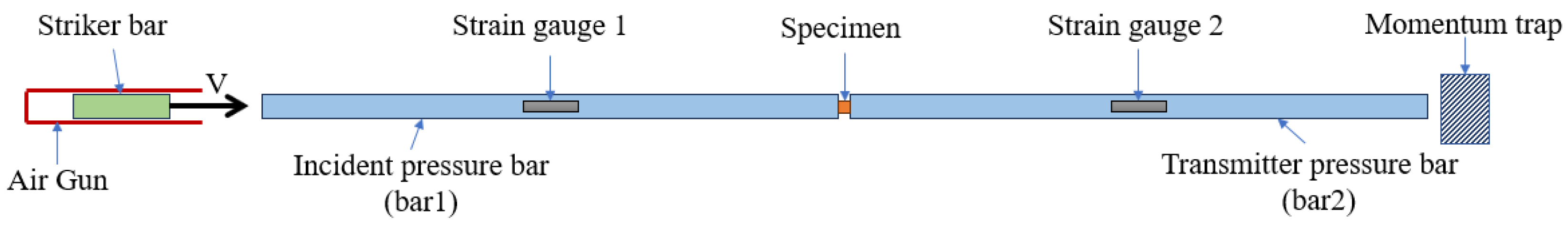
The SHPB experiments conducted in this study were simulated to verify the correctness of the J-C model constants obtained from the experimental findings. For this purpose, first, the tensile testing apparatus was used to determine the strength of the material at a strain rate of 0.001 s
−1. This test’s outcomes contributed to calculating the J-C coefficients A, B, and n. Also, a schematic of Hopkinson’s test is shown in
Figure 3 [
28,
29].
Based on the calculations thoroughly presented in the literature from the measured strain in the first and second bars, the actual strain rate, strain, and stress developed in the test specimen were calculated [
29]. The strain rate sensitivity constant, C, was calculated from the J-C estimate based on the true stress and strain results extracted in Hopkinson’s tests at different velocities and strain rates. The values of the J-C material constants for the AA5052-H34 and WC are given in
Table 3 [
21].
Utilizing the J-C equation formulated for the AA 5052-H34, the corresponding stress and strain curves at varying strain rates are illustrated in
Figure 4. The uniaxial tensile test data depicted in this diagram, which have an average strain rate of 0.001 s
−1, align well with the stress derived from the Johnson–Cook equation at an identical strain rate. The impact of strain rate augmentation on hardening is distinctly observable. However, it is noteworthy that the pace at which the AA 5052-H34 strength increases tends to diminish at elevated strain rates. In other words, as the strain rate escalates, the intensity of the hardening induced by the strain rate lessens. Also, the increase in the stress value from the reference strain rate and the quasi-static state to the dynamic state with a strain rate of 100,000 (1/s) is about 40 MPa. The discrepancy in these stress values indicates the medium sensitivity of AA 5052-H34’s dynamic behavior to the strain rate.
Figure 5 depicts the strain measured by the strain gauges of bar 1 and bar 2 in the experimental test with the speed of throwing the striking bar towards bar 1 equal to 14.65 m/s, and the strain values obtained from the simulation of the test process with this speed are also depicted. The correspondence of the two diagrams in this figure clearly shows the accuracy of the simulated material model.
The diagram in
Figure 6 shows the impact of varying striker bar speeds on the maximum true stress in the sample material. This stress is determined based on the FE simulation. The calculated results from the practical Hopkinson tests are also shown with a measurement error of 5% assumed in these tests. These results clearly show a good match between the experimental and simulation results of the material model for the SHPB test. Based on this, it can be stated that the AA 5052-H34 used in this work has been modeled in an acceptable way using Johnson Cook’s constitutive equation and can be used in machining simulation.
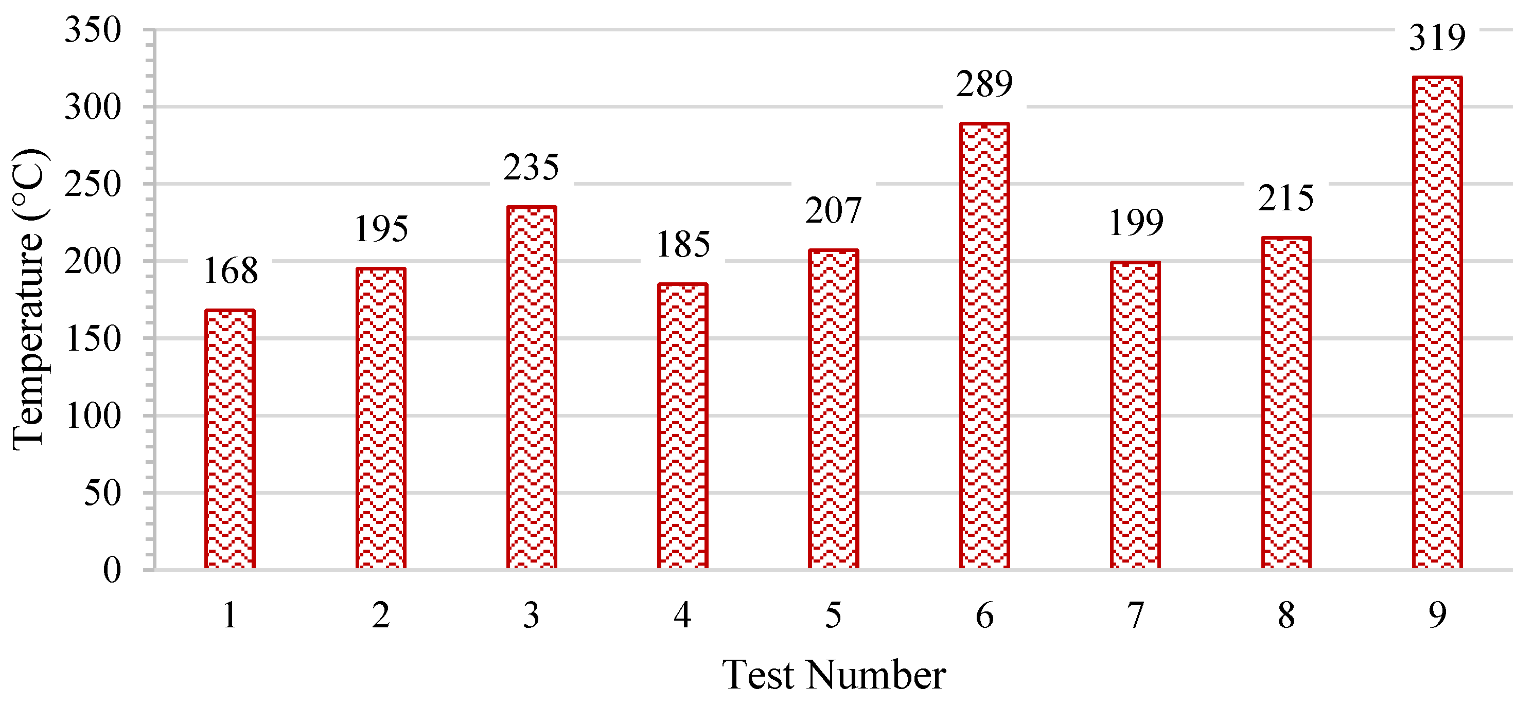
Figure 7 shows the maximum temperature diagram estimated in the simulation of the Hopkinson test at different launch speeds. In all these tests, the initial temperature of the sample is considered equal to 25 °C. As can be seen, due to the increase in kinetic energy and as a result, the energy transferred when hitting bar 1 of the Hopkinson test increases the plastic stress created in the specimen and the heat generated resulting from the deformation produced in the sample.
A damage model, capable of characterizing material behavior upon damage, is incorporated in the FEM simulation to study the formation of chips. The J-C failure model was used as a criterion for damage initiation. This model is grounded on the equivalent plastic strain at failure, denoted as
. The definition of
is as follows [
16]:
where
and
represent compressive stress and von Mises stress, respectively. The damage constants of the Johnson-Cook damage are also D1-D5. The damage initiation threshold is modeled in Abaqus/Explicit version 2021according to a cumulative damage law [
16]:
where
is the increment of the equivalent plastic strain.
Based on the recent relationships, results from the SHPB simulation tests, and initial simulations of the machining process, it is assumed that the values of the J-C damage parameters are equivalent to those presented in
Table 4.
The accuracy of the plasticity model and the damage model estimated in this study were investigated using machining process simulation.
2.2. Experimental Tests
The dry-turning setups used in this research are shown in
Figure 8. The experimental machining work was conducted using a Mori Seiki SL-15 CNC lathe machine, which is renowned for its precision and reliability. This series, first manufactured in 1989, is equipped with a swing-over bed of 17.7 inches and a machining length of 23.4 inches. It features a 6-position turret, allowing a wide range of machining operations.
A Fanuc Series 15-T system controls the Mori Seiki SL-15. This control system is part of the Fanuc 15 series, known for its versatility across different types of machines. Fanuc Series 15-T provides detailed instructions and guides for using and maintaining the control system, ensuring optimal performance of the CNC machine. In case of any alarms, errors, or faults, the system provides specific codes to help identify and rectify the issue. In machining tests, a PSBNL 2020 K12 holder and SCGT120408-LHC inserts were fabricated by the CDBP company.
Two cylindrical workpieces with a length of 250 mm and a diameter of 50 mm were used for turning tests. Both workpieces, made of AA5052-H34, were prepared for the machining process. Grooves were meticulously carved at uniform intervals of 50 mm and adjusted for dimensional precision. The chip morphology was analyzed with an optical microscope with a maximum of 120× magnification. The surface roughness was measured with a MAHR roughness gauge.
The design of experiments (DoE) for this work was performed using the multilevel factorial method in Statgraphics version 19 software. The multilevel factorial DoE is a statistical technique that explores the influence of various factors on an outcome. This method permits the simultaneous variation of all factor levels, facilitating the investigation of factor interactions. The process involves the identification of factors. It also consists of setting levels for each factor. However, it can be challenging with many factors or levels, and errors can compromise the study. Given the article’s subject, the limited parameter range, and the focus on chip morphology, a two-factor three-level design of nine tests was chosen for its simplicity and precision. These nine cutting conditions involved three levels of cutting speed and three levels of feed rate at a constant depth of cut.
As shown in
Table 5 the experimental investigation was conducted considering three levels for two cutting parameters; the cut depth was also consistently maintained at 1 mm. The simulation angles were also derived from the embedded angles in the holder and insert. According to the common values in the machining of aluminum alloys, the positive side rake angle is recommended to be between 10 and 20 degrees, and according to the available equipment, a fixed value of 13 degrees was used in all experimental and numerical tests. Also, the cutting speed and feed rate selections were performed based on the machinery’s handbook recommendation, the range of morphology change reported in previous research for similar alloys, and the parameters proposed by the tool manufacturing company [
22,
30].


