Thermomechanical Analysis of PBF-LB/M AlSi7Mg0.6 with Respect to Rate-Dependent Material Behaviour and Damage Effects

Abstract

This paper describes the self-heating effects resulting from mechanical deformation in the additively manufactured aluminium alloy AlSi7Mg0.6. The material’s self-heating effect results from irreversible changes in the material’s microstructure that are directly coupled with the inelastic deformations. These processes are highly dissipative, which is reflected in the heat generation of the material. To describe such effects, a numerical framework that combines an elasto-viscoplastic Chaboche model with the Gurson Tvergaard Needleman damage approach is analysed and thermomechanically extended. This paper characterises the sample preparation, the experimental set-up, the development of the thermomechanical approach, and the material model. A user material subroutine applies the complete material model for the finite element software Abaqus 2022. To validate the material model and the parameters, a complex tensile test is performed. In order to check the finite element model, the energy transformation ratio is included in the evaluation. The numerical analyses of the mechanical stress evolution and the self-heating behaviour demonstrate good agreement with the experimental test. In addition, the calculation shows the expected behaviour of the void volume fraction that rises from the initial value of $0.0373\%$ to a higher value under a complex mechanical load.

1. Introduction

The microstructure of a metal strongly depends on the type of alloy. It depends on its chemical composition, processing method, and final post-processing treatment. These factors lead to wide variability in the microstructure and, in fact, in the properties of the material. For one type of material, e.g., steels, the microstructure can have a different matrix of phases and precipitations, even for the same chemical composition, but it depends on the applied processing technique [1].

Additive manufacturing processes enable a cost-efficient production of components and small series with complex structures and reduce the number of individual parts and assembly steps. Applications for this additive manufacturing include aerospace [2], medical technology [3], tool manufacturing [4], and energy technology [5]. In the field of metal component fabrication, the laser powder bed fusion of metals (PBF-LB/M) process and the direct energy deposition (DED) method are the most established techniques [6,7]. In comparison to the well-known conventional fabrication methods such as cast moulding, additive manufacturing, especially PBF-LB/M, results in an extremely fine-grained microstructure obtained for almost each processed material [8]. It is the result of a specific process with high heating/cooling rates and high temperature gradient. However, due to the above-mentioned factors, the material in the as-built state is characterised by a high level of residual stress, which, in turn, translates into mechanical properties [9]. Usually, PBF-LB materials are characterised by a high level of tensile strength and a middle/low level of plasticity. Therefore, it is highly recommended to use a post-process heat treatment to relax the residual stresses and make the properties uniform across the entire specimen [9]. The following factors influence the quality of the final product made by PBF-LB/M: microstructure, porosity, residual stresses, dimensional accuracy, and surface roughness [10,11]. Some of these factors are derived from the process parameters, while adding post-process thermal and/or mechanical treatments additionally affects the obtained material characteristics.

In the case of aluminium alloys, and especially, the series 4xxx, AM users and researchers are dealing with Al-Si eutectics, which exhibit good fluidity and allow for a crack-free PBF-LB/M solidification [12]. Compared to casting methods, AlSi7Mg0.6 alloy in the as-built state (PBF-LB) achieves a tensile strength of about 390 MPa, yield strength of 210 MPa, and an elongation of about 8% [12,13]. These values significantly exceed the characteristics obtained with casting [14] and result from rapid solidification in the PBF-LB/M process, which was mentioned above. Aluminium alloys in the as-built state have a similar microstructure as conventional materials after supersaturated solution heat treatment. It is highly possible that after ageing, those materials will achieve higher tensile strength, but with noticeable lower ductility [10].

To enable the additively manufactured materials as construction components, the behaviour of the material under mechanical loads needs to be predicted. The studies of [15] has shown that an elasto-viscoplastic thermomechanical material model [16] can represent the AlSi7Mg0.6 alloy behaviour with some limitations. Differences between the experiment and simulation are visible at two phenomena. The first is in the region of the yield point, where the material behaviour changed from elastic to inelastic. And the second limitation focuses on the phenomena of stress relaxation. Due to the presence of stress relaxation, a rate-dependent material behaviour of AlSi7Mg0.6 was detected. Consequently, rate-independent models, as in [17], are excluded for the numerical description. In order to reduce the limitations in the representation of the addressed phenomena, more complex rate-dependent models such as [18,19] can be implemented. Both models operate on the assumption of a nearly homogeneous material structure. In the case of additive manufacturing, the resulting inhomogeneous material structure has a significant influence on the mechanical properties. To include the influence of the microstructure on the mechanical properties of the material in numerical modelling, damage models exist that describe the defect in terms of pore phenomena. An example of modelling void growth, void nucleation, and void coalescence is provided by the Gurson–Tvergaard–Needleman (GTN) damage model [20,21,22]. This damage approach represents a rate-independent material behaviour but may be extended by modifications to the rate-dependent model. For polymers, an approach exists which combines a classical continuum mechanical model with consideration of damage effects [23]. In this study, the elasto-viscoplastic Chaboche model [19] was connected with the Gurson–Tvergaard–Needleman damage model. The authors of [23,24] investigated and verified the ability of the material model to predict the failure behaviour. A description of the material behaviour is performed by a system of differential equations. The solution of such numerical problems results in an optimisation task that describes the initial and boundary value challenge. In the classical approach, mechanical stress is considered as an objective. The temperature evolution on the sample surface can be integrated into the solution as a second objective function, as the system is thermodynamically enhanced. In conclusion, the thermomechanical analysis can provide a numerical optimisation task [15,25,26].

The continuum thermomechanics considers the entire deformation process as a thermodynamical system [27]. As a result of the dissipative hardening processes, the self-heating of the material is described by observing the first two laws of thermodynamics [28,29]. To calculate the change in the material surface, the dissipation energy can be separated into mechanical strain energy and the energy that is necessary to change the microstructure of the material [30]. The last energy part is known as the stored energy of cold work [31]. This provides a good approach, which results in an efficient optimisation task for the coupled field problem of stress behaviour and self-heating of the material [16,17,32,33].

This study focuses on the material description of the PBF-LB/M-manufactured AlSi7Mg0.6 alloy with respect to the rate-dependent material behaviour and damage effects. To create a more detailed analysis, a Chaboce-GTN model [23] is enhanced from the point problem to the three-dimensional FE-problem. The use of the damage approach results in a numerical consideration of the pore phenomena (growing, nucleation, and coalescence) [22]. To determine the initial parameters of the GTN model, the microstructure analysis is presented. For a more precise objective function in the optimisation task, the model is extended by the first and second law of thermodynamics. This approach results in the stress–strain, the temperature, and the energy transformation ration material characteristics for one experimental scenario. To develop the coupled stress–temperature field problem of thermomechanics for the optimisation task, concepts for combined experimental investigations and theoretical model extensions [34] are integrated into the research.

2. Materials and Methods

2.1. Additive Manufacturing of Aluminium Alloys

The test specimens were made from AlSi7Mg0.6 alloy powder with a fractional distribution of 20–63 $\mathsf{\mu }$m, supplied by the machine manufacturer, SLM 280 2.0 (SLM Solutions Group AG, Lübeck, Germany). The dog bone flat samples, with a thickness of 1.5 mm and dimensions according to DIN50125-H12.5 × 50, were printed in the vertical orientation, with a remelted powder layer thickness of 30 $\mathsf{\mu }$m. The set of process parameters recommended by the machine supplier was used to produce the samples. Therefore, the material relative density of no less than 99.8% is to be achieved. The total number of samples made per process was 16 pcs (Figure 1). The samples tested in the research were in the as-built condition, i.e., no post-process heat treatment was applied. A complete characterization of the powder used in this study and the material obtained from the PBF-LB/M process can be found in [35].

2.2. Microstructure Analysis

This study was performed using the X-ray computer tomography (XCT) system Waygate phoenix|v|tome|× 300 m (Baker Hughes Company Houston/Texas), scanning samples before and after the tensile test with the same measurement parameters. The voxel size was 7 $\mathsf{\mu }$m, the voltage and current of the X-ray tube were 220 kV and 30 $\mathsf{\mu }$A, respectively. For each scan, 2700 projections were collected with an integration time of 150 us, using a 0.5 mm copper filter. Porosity analysis was performed using software VG Studio MAX 3.3 (Volume Graphics GmbH, Heidelberg, Germany). The results show the mean value of six samples. In the case of the virgin samples, the initial void volume fraction ${\widehat{f}}^{*}$ is $0.0373$%. After the thermomechanical experiments, ex situ analyses were performed on the damaged samples. This analyses leads to the critical damage void volume fraction ${\widehat{f}}^F$ with $0.0385$%. For more details about the material’s porosity, see [35].

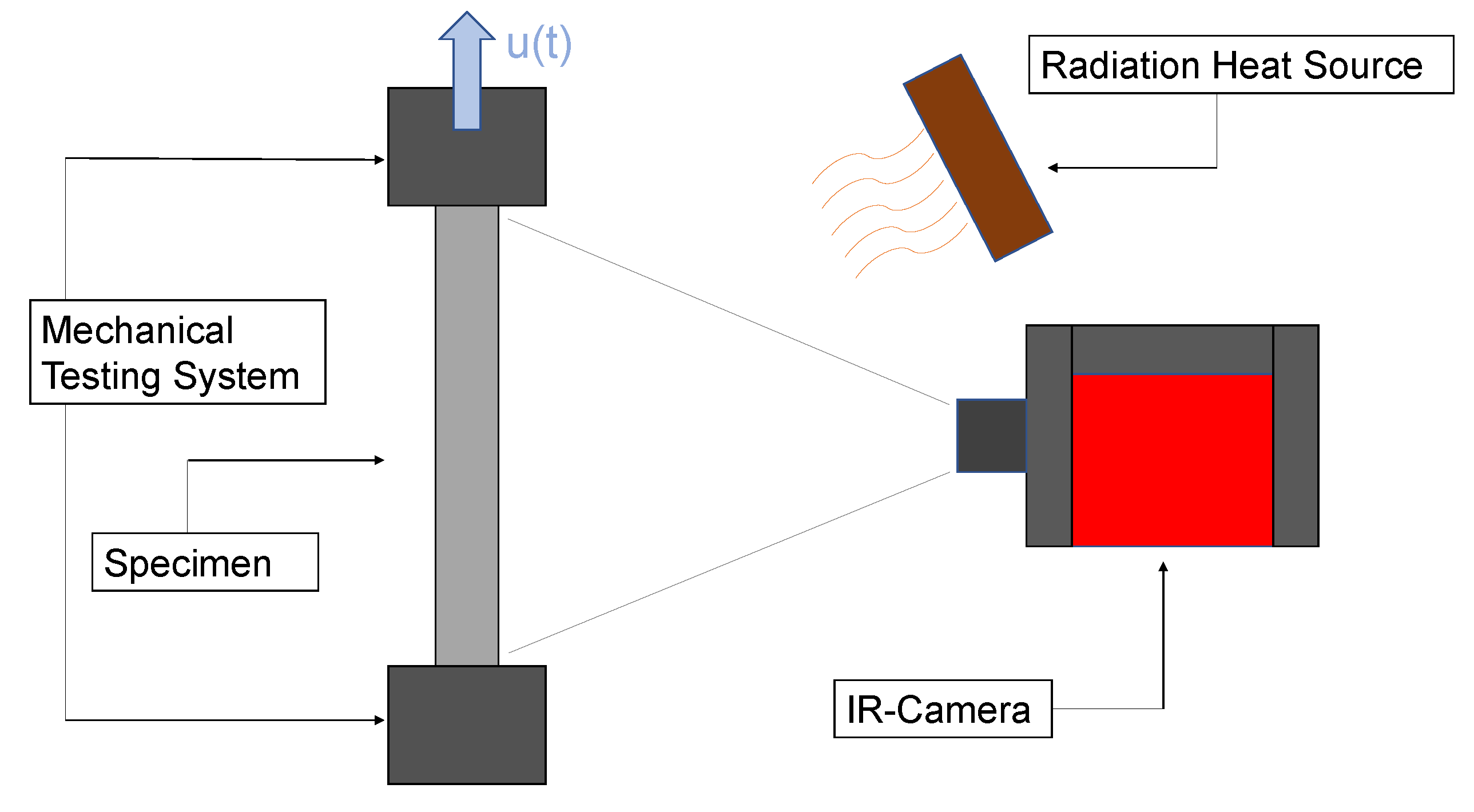
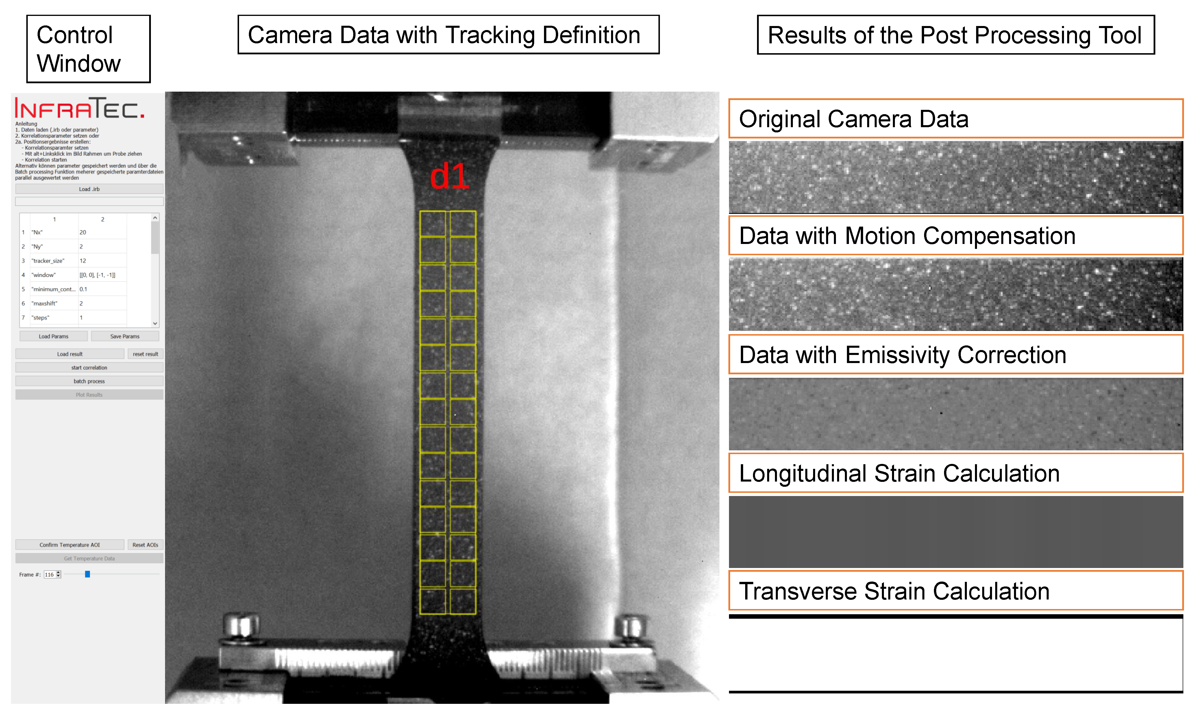
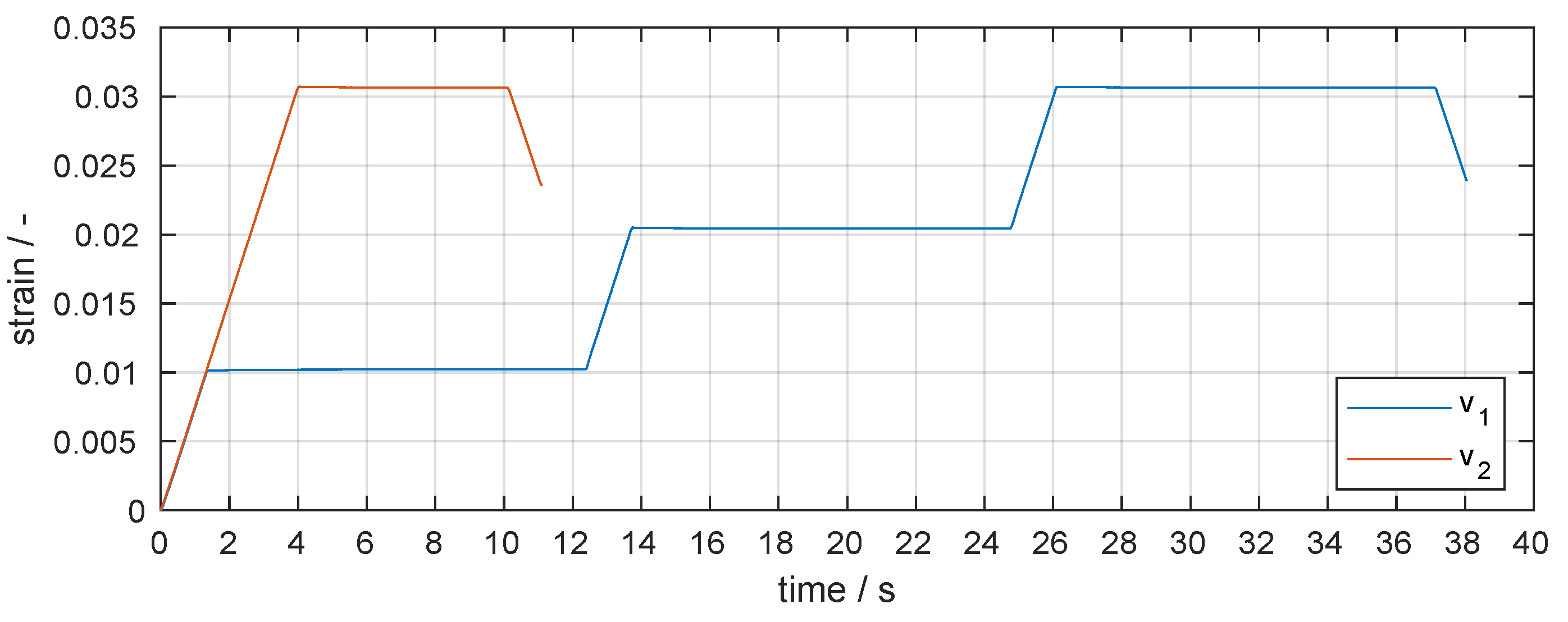
2.3. Thermomechanical Experiment

The determination of the mechanical and thermal material behaviour is performed by the thermomechanical experiment. To simplify the measurement configuration, a specific experimental set-up was used, as shown in Figure 2.

The complex tensile tests were conducted using a servo-hydraulic test machine from the company Zwick & Roell (Ulm, Germany) If country is USA, please provide state after city. with a maximum load cell of 25 kN. The deformation and temperature field were measured in a coupled process realised with the infrared camera ImageIR 8300 hs from InfraTec GmbH (Dresden, Germany). If country is USA, please provide state after city.

Table 1. Specifications of the ImageIR 8300 hs.

Property/Parameter	Unit	Specification
Sensor		T2SLS with Hot Long-Life-Technologie
Detector format	(px) × (px)	640 × 512
Pitch size	$\mathsf{\mu }$m	25
Spectral region	$\mathsf{\mu }$m	$1.5\dots 5.5$
Temperature resolution at 30 °C measuring range	mK	20
Measuring range	°C	$-40\dots 1500$
IR frame rate	Hz	125
Distance to Specimen	mm	300

shows the technical specifications of the used IR-camera.

To measure the deformation field, a digital image correlation (DIC) is implemented. For a high-quality temperature measurement without reflections of the surrounding radiations, the samples are sprayed with a black matte varnish. The reference points for the DIC are created with a random dot pattern. This pattern is realised with a spray that includes metallic particles and generates local emissivity differences and creates reference points for the DIC. The resulting thermal contrast increases with an external continuous radiation heat source. Detailed specifications for the experimental set-up, the sample preparation, and the analysis are described in [15,34,36].

The deformation field was calculated using a post-processing tool from InfraTec. The user interface is shown in Figure 3. To begin the process, the user can define tracker points on a sub-surface for the DIC (Figure 3(d1)). The tool loads the original camera data first. In order to realise the temperature measurement, a motion compensation is implemented and an emissivity correction is performed. These steps eliminate the noise of the temperature signal. The tool uses an affine transformation to calculate the deformations. After processing, the user can choose between the longitudinal strain data in the tension direction and the transverse strain data. For more details about the post-processing tool, see [36]. In a final step, the result files are generated at defined points or as a mean value of a sub surface. In this paper, the following material curves are created in the midpoint of the detail d1 in Figure 3.

Motivated by the ASTM E328-20 standard [37], a modified complex load path ${\mathrm{v}}_1$ was selected for parameter identification, verification, and the resulting optimisation task. In this case, complex means that multiple holding times on different strain levels were integrated in the tensile test. There is an additional unloading path for the verification of the elastic material behaviour. This unloading means that the test ends without destroying the sample. In order to satisfy the assumptions of the thermomechanical approach, a displacement-controlled experiment with a strain rate of $\dot{\mathit{\epsilon }}=7.7·{10}^{-3}$ ${\mathrm{s}}^{-1}$ was performed. For the validation of the parameters determined by ${\mathrm{v}}_1$, a second load path ${\mathrm{v}}_2$ is defined. This experiment involves a uniaxial tension to a maximum strain of $3.06$%, with a following holding time at this strain level of 6 s and a final unloading. The strain rate of ${\mathrm{v}}_2$ is the same as ${\mathrm{v}}_1$. All experimental characteristics (strain, stress, and temperature evolution) shown in this work are the mean value curves of the six tested samples. A definition of both loading paths is shown in Figure 4.

The post-processing tool evaluates the thermomechanical experiments. This involves the local analysis of the material behaviour at the midpoint of the specimen (see detail d1 in Figure 3). Figure 5A,C present the thermomechanical material response for the load path of ${\mathrm{v}}_1$. The diagrams show three test curves and the mean value curve for a better understanding. For the stress curve and the temperature curve, the standard deviation is $S_{\mathit{\sigma }}=\pm 1.73\%$ and $S_{\Theta }=\pm 0.58\%$. In the case of the load path ${\mathrm{v}}_2$, the thermomechanical material response is presented in Figure 5B,D. The standard deviation of the stress curve amounts to $S_{\mathit{\sigma }}=\pm 1.1\%$ and of the temperature curve amounts to $S_{\Theta }=\pm 0.74\%$. Both test scenarios are finally employed for the optimisation task to determine the parameters of the selected material model.

2.4. Theoretical Framework

A large number of theoretical approaches are available for the numerical representation of mechanical material behaviour [27]. Some theoretical concepts differentiate between rate-dependent [16] and rate-independent [17] material behaviours [19] introduces a model that can represent a large number of material phenomena (like rate dependency, isotropic hardening, kinematic hardening, etc.). The increasing importance of additively manufactured components as construction materials leads to additional phenomena that are characterised by the damage of the material during the loading process. Consequently, mechanical properties are becoming important for the quality of the final microstructure [14]. For this reason, there are concepts that couple the Chaboche model with damage approaches [23]. This coupling leads to a complex model with a large number of determinable parameters. In order to obtain more information from a single test scenario, the model is extended thermomechanically. Based on the enhancement, the temperature curves generated by the material’s self-heating effects in addition to the stress–strain curves are used for parameter identification [15,25,26]. Motivated by this approach, the following sections explain the thermomechanical model.

2.4.1. Dissipation

Before the thermomechanical approach is discussed, the mechanical system is limited to the technically relevant range of small deformations. Consequently, the norm of the displacement gradient tensor is much smaller than 1, and the deformation can be described by the linearised deformation–displacement relation.

The theory describes the evolution of the internal variables of the chosen model in terms of the material hardening phenomenon [27]. Such inelastic effects are caused by changes in the microstructure, which describes a highly dissipative process. To define the problem of self-heating, an expression for dissipation energy is required first. This procedure assumes a homogeneous temperature distribution over the thickness of the sample, a fact that is given by the small thickness of the sample. Combining the first and second laws of thermodynamics results in dissipation inequality:

$$\Delta =\Theta \dot{s}-\dot{e}+{\displaystyle \frac{1}{\rho }}\mathit{\sigma }:\dot{\mathit{\epsilon }}-{\displaystyle \frac{1}{\rho \Theta }}\mathit{q}:\mathit{g}\ge 0,$$

(1)

where the internal dissipation is $\Delta$, the sample surface temperature is $\Theta$, the entropy rate is $\dot{s}$, the specific free energy rate is $\dot{e}$, the mass density is $\rho$, the Cauchy stress tensor is $\mathit{\sigma }$, the linearised Green-Lagrange strain tensor rate is $\dot{\mathit{\epsilon }}$, the specific heat flux vector is $\mathit{q}$, and the temperature gradient is $\mathit{g}$.

The evolution of internal energy $\dot{e}$ depends on changes in the entropy $\dot{s}$ and the strain tensor $\dot{\mathit{\epsilon }}$, as shown in Equation (1). The entropy is defined as a measure of the irreversibility of the system [27]. Because the challenges for the experimental evidence of entropy are very difficult, the system is described by a different thermodynamic potential. With the Legendre transformation $\psi =e-\Theta s$, the system is considered as a function of free energy $\psi$ as follows:

$$\Delta =-s\dot{\Theta }-\dot{\psi }+{\displaystyle \frac{1}{\rho }}\mathit{\sigma }:\dot{\mathit{\epsilon }}-{\displaystyle \frac{1}{\rho \Theta }}\mathit{q}:\mathit{g}\ge 0.$$

(2)

Before discussing the dependencies of the free energy potential more in detail, two assumptions are defined:

• Temperature strain ${\mathit{\epsilon }}^{th}$ is negligible;
• The viscoplastic strain is an internal variable [38].

The first assumption deals with the fact that the temperature changes resulting from self-heating are very small. For this reason, the temperature strain ${\mathit{\epsilon }}^{th}$ compared with the mechanical strain is very small and negligible. With the restriction to small deformations, the strain tensor $\mathit{\epsilon }$ is described by the sum of the elastic strain tensor ${\mathit{\epsilon }}^{el}$ and the viscoplastic strain tensor ${\mathit{\epsilon }}^{vp}$.

$$\begin{array}{cc}\hfill \mathit{\epsilon }& ={\mathit{\epsilon }}^{th}+{\mathit{\epsilon }}^{el}+{\mathit{\epsilon }}^{vp}\hfill \\ \hfill {\mathit{\epsilon }}^{el}& =\mathit{\epsilon }-{\mathit{\epsilon }}^{vp}\mathrm{with}{\mathit{\epsilon }}^{th}=\mathbf{0}.\hfill \end{array}$$

(3)

The second assumption introduces the viscoplastic strain as an internal variable [38]. With these aspects, the free energy applies the following:

$$\Psi =\Psi \left({\mathit{\epsilon }}^{el},\Theta ,\mathit{g},{\mathit{a}}^1,\dots ,{\mathit{a}}^n\right),$$

(4)

where ${\mathit{a}}^1,\dots ,{\mathit{a}}^n$ are thermodynamic displacements, which represent the mechanical strain type internal variables in the thermomechanical framework. Considering Equations (3) and (4) in Equation (2) leads to the following:

$$\begin{array}{c}\hfill \Delta =\left({\displaystyle \frac{1}{\rho }}\mathit{\sigma }-{\displaystyle \frac{\partial \psi }{\partial {\mathit{\epsilon }}^{el}}}\right)\dot{\mathit{\epsilon }}+\left(-s-{\displaystyle \frac{\partial \psi }{\partial \Theta }}\right)\dot{\Theta }+{\displaystyle \frac{\partial \psi }{\partial {\mathit{\epsilon }}^{el}}}{\dot{\mathit{\epsilon }}}^{vp}\\ \hfill -\sum _{j=1}^n\left({\displaystyle \frac{\partial \psi }{\partial {\mathit{a}}^j}}{\dot{\mathit{a}}}^j\right)-{\displaystyle \frac{\partial \psi }{\partial \mathit{g}}}\dot{\mathit{g}}-{\displaystyle \frac{1}{\rho \Theta }}\mathit{q}:\mathit{g}\ge 0.\end{array}$$

(5)

To analyse the dissipation inequality (5), the meaning of the equation first needs to be explained. The thermodynamic system is reversible when this expression is equal to zero. Reversible means that the system can return to its initial state [27]. An example of this are adiabatic elastic processes. When the inequality is greater than zero, the process is irreversible. Consequently, the system is unable to return to its initial state. This condition is characterised by inelastic deformation processes and heat conduction. In order to evaluate Equation (5), it is common practice to focus on reversible processes first [39]. The dissipation inequality results in the following:

$$\begin{array}{c}\hfill \Delta =\left({\displaystyle \frac{1}{\rho }}\mathit{\sigma }-{\displaystyle \frac{\partial \psi }{\partial {\mathit{\epsilon }}^{el}}}\right){\dot{\mathit{\epsilon }}}^{el}+\left(-s-{\displaystyle \frac{\partial \psi }{\partial \Theta }}\right)\dot{\Theta }-{\displaystyle \frac{\partial \psi }{\partial \mathit{g}}}\dot{\mathit{g}}-{\displaystyle \frac{1}{\rho \Theta }}\mathit{q}:\mathit{g}=0.\end{array}$$

(6)

Equation (6) is thermomechanically consistent when each sum and satisfies the mathematical expression [39]. For the last sum and Equation (6), the Fourier equation of the heat flow $\mathit{g}$ can be used [16]:

$$\mathit{q}=-k\mathit{g},$$

(7)

where the thermal conductivity is k. Considering Equation (7) and in the case of adiabatic boundary conditions, the temperature gradient $\mathit{g}$ becomes zero, and Equation (6) is satisfied. All other summands solve the equation whenever the following is valid:

$$\mathit{\sigma }=\rho {\displaystyle \frac{\partial \psi }{\partial {\mathit{\epsilon }}^{el}}},s=-{\displaystyle \frac{\partial \psi }{\partial \Theta }}\mathrm{and}{\displaystyle \frac{\partial \psi }{\partial \mathit{g}}}=0.$$

(8)

The Coleman and Noll approach (Equation (8)) has been established for irreversible processes to [38]. Embedding Equation (8) in Equation (5) results in the following:

$$\Delta =\underset{e^{vp}}{\underbrace{{\displaystyle \frac{1}{\rho }}\mathit{\sigma }:{\dot{\mathit{\epsilon }}}^{vp}}}-\underset{e^s}{\underbrace{\sum _{j=1}^n{\displaystyle \frac{\partial \psi }{\partial {\mathit{a}}^j}}:{\dot{\mathit{a}}}^j}}-{\displaystyle \frac{1}{\rho \Theta }}\mathit{q}:\mathit{g}\ge 0.$$

(9)

Equation (9) describes the dissipation structure for an inelastic system. The inelastic deformation process introduces a viscoplastic stress power $e^{vp}$ into the system. As the material hardening in the inelastic range results in a change in the material’s microstructure [27], the entire stress power is not dissipated. The stored energy of cold work $e^s$ defines the energy part that is responsible for the changes in the microstructure. These two terms are often called intrinsic dissipation ${\delta }^{intr}$. The third term of Equation (9) is known as the thermal dissipation ${\delta }^{th}$ [38]. The chosen material model [23] describes the evolution of the internal variables in the stress area. As the free energy in Equation (4) is a function of strain space values, it is more consistent to describe the thermomechanical system in terms of the free enthalpy G [17]. With the Legendre transformation $\Psi ={\displaystyle \frac{1}{\rho }}\sigma :{\epsilon }^{el}-G$, the dissipation inequality (2) reads to the following:

$$\Delta =-{\displaystyle \frac{1}{\rho }}{\mathit{\epsilon }}^{el}:\dot{\mathit{\sigma }}+\dot{G}-s\dot{\Theta }+{\displaystyle \frac{1}{\rho }}\mathit{\sigma }:{\dot{\mathit{\epsilon }}}^{vp}-{\displaystyle \frac{1}{\rho \Theta }}\mathit{q}:\mathit{g}\ge 0.$$

(10)

Now, the following dependencies take effect for the free enthalpy as follows:

$$G=G\left(\mathit{\sigma },\Theta ,\mathit{g},{\mathit{A}}^1,\dots ,{\mathit{A}}^n\right),$$

(11)

where ${\mathit{A}}^1,\dots ,{\mathit{A}}^n$ are the thermodynamic forces. With Equation (11), the dissipation inequality (10) follows the below equation:

$$\begin{array}{c}\hfill \Delta =\left({\displaystyle \frac{\partial G}{\partial \mathit{\sigma }}}-{\displaystyle \frac{1}{\rho }}{\mathit{\epsilon }}^{el}\right)\dot{\mathit{\sigma }}+\left({\displaystyle \frac{\partial G}{\partial \Theta }}-s\right)\dot{\Theta }+{\displaystyle \frac{1}{\rho }}\mathit{\sigma }:{\dot{\mathit{\epsilon }}}^{vp}\\ \hfill +\sum _{j=1}^n{\displaystyle \frac{\partial G}{\partial {\mathit{A}}^j}}{\dot{\mathit{A}}}^j-{\displaystyle \frac{\partial G}{\partial \mathit{g}}}\dot{\mathit{g}}-{\displaystyle \frac{1}{\Theta }}\mathit{q}:\mathit{g}\ge 0.\end{array}$$

(12)

After the evaluation of Equation (12) for reversible processes, the potential relationships are determined by the Coleman Noll procedure:

$${\mathit{\epsilon }}^{el}=\rho {\displaystyle \frac{\partial G}{\partial \mathit{\sigma }}},s={\displaystyle \frac{\partial G}{\partial \Theta }},{\displaystyle \frac{\partial G}{\partial \mathit{g}}}=0.$$

(13)

Implementing Equation (13) in Equation (12) results in the dissipation inequality for irreversible processes as follows [27]:

$$\Delta =\underset{e^{vp}}{\underbrace{{\displaystyle \frac{1}{\rho }}\mathit{\sigma }:{\dot{\mathit{\epsilon }}}^{vp}}}-\underset{e^s}{\underbrace{\sum _{j=1}^n{\displaystyle \frac{\partial \psi }{\partial {\mathit{A}}^j}}:{\dot{\mathit{A}}}^j}}-{\displaystyle \frac{1}{\rho \Theta }}\mathit{q}:\mathit{g}\ge 0.$$

(14)

2.4.2. Energy Transformation Ratio

It is possible to characterise the dissipative behaviour of the materials in terms of the energy transformation ratio (etr). To derive this quantity, the consideration of dividing the intrinsic dissipation ${\delta }^{intr}$ into a ratio of the viscoplastic stress power $e^{vp}$ and a ratio of the stored energy of cold work $e^s$ leads to the determination of energy ratios based on the system [17]. For this case, the viscoplastic work $w^{vp}$ is defined as follows:

$$w^{vp}={\int }_{t_0}^t{e}^{vp}\mathrm{d}\overline{t}.$$

(15)

According to the same procedure, the cold work of stored energy $w^s$ is defined as follows:

$$w^s={\int }_{t_0}^t{e}^s\mathrm{d}\overline{t}.$$

(16)

As a result, the dissipative character of the material can be represented by the etr $\phi$ due to the ratio between the cold work of stored energy $w^s$ and the viscoplastic work $w^{vp}$ [16] as follows:

$$\phi ={\displaystyle \frac{w^s}{w^{vp}}}.$$

(17)

2.4.3. Heat Equation

Heat equation is an important part of thermomechanics, as well as the calculation of system’s dissipation. For this purpose, the first law of thermodynamics is formulated according to the following:

$$\dot{e}=-{\displaystyle \frac{1}{\rho }}\left(\mathit{q}\right)+r+{\displaystyle \frac{1}{\rho }}\mathit{\sigma }:\dot{\mathit{\epsilon }}.$$

(18)

In order to represent the increase in temperature as a result of dissipation, the entropy balance of the system is generally analysed. To define the entropy balance for free enthalpy, the Gibbs relation is used [27]:

$$\dot{G}={\displaystyle \frac{1}{\rho }}\mathit{\epsilon }:\dot{\mathit{\sigma }}+s\dot{\Theta }.$$

(19)

With the Legendre transformations of free enthalpy G in free energy $\psi$ to internal energy e and the implementation in Equation (18), the entropy balance follows the below equation:

$$\Theta \dot{s}=-{\displaystyle \frac{1}{\rho }}\left(\mathit{q}\right)+r.$$

(20)

Evaluating the potential of entropy based on Coleman Noll’s consequences, Equation (13) results in the following heat conduction equation:

$$\underset{c^{\sigma }}{\underbrace{\Theta {\displaystyle \frac{{\partial }^2{G}^{el}}{\partial {\Theta }^2}}}}\dot{\Theta }=-\underset{e^{el}}{\underbrace{\Theta {\displaystyle \frac{{\partial }^2{G}^{el}}{\partial \Theta \partial \mathit{\sigma }}}}}\dot{\mathit{\sigma }}+\underset{e^{vp}}{\underbrace{{\displaystyle \frac{1}{\rho }}\mathit{\sigma }:{\dot{\mathit{\epsilon }}}^{vp}}}-\underset{e^s}{\underbrace{\Theta \sum _{j=1}^n\left[{\displaystyle \frac{{\partial }^{2}G}{\partial \Theta \partial {\mathit{A}}^j}}{\left({\displaystyle \frac{\partial G}{\partial {\mathit{A}}^j}}\right)}^{.}\right]}}-\underset{e^Q}{\underbrace{{\displaystyle \frac{1}{\rho }}\left(\mathit{q}\right)+r}},$$

(21)

where $G^{el}$ is the elastic part of the free enthalpy, $c^{\sigma }$ is the specific heat for the constant stress case [27], $e^{el}$ describes the thermoelastic effect, and $e^Q$ defines the heat conduction process, including the heating by an external heat source. For the determination of elasto-plastic material behaviour, the thermoelastic effect is defined more accurately. In the case of tension, the sample cools down; and in the case of compression, the sample heats up [16]. To describe this effect numerically, a linear Hooke’s thermoelasticity is applied as follows [38]:

$$\rho G^{el}={\displaystyle \frac{1}{2}}{\displaystyle \frac{1}{2\mu }}{\mathit{\sigma }}^D:{\mathit{\sigma }}^D+{\displaystyle \frac{1}{2}}{\displaystyle \frac{1}{9\kappa }}{\left(\mathrm{tr}\left(\mathit{\sigma }\right)\right)}^2+{\alpha }^0\left(\mathrm{tr}\left(\mathit{\sigma }\right)\right)\left(\Theta -{\Theta }^0\right)+{\displaystyle \frac{\rho }{2}}{\displaystyle \frac{c^{\sigma }}{{\Theta }^0}}{\left(\Theta -{\Theta }^0\right)}^2,$$

(22)

where the shear modulus is $\mu$, the bulk modulus is $\kappa$, the thermal expansion coefficient is ${\alpha }^0$, the elastic strain deviator is ${\mathit{\epsilon }}^{elD}$, and the reference temperature is ${\Theta }^0$.

2.4.4. Material Model

The combined Chaboche-GTN model was selected to describe the material behaviour numerically. In previous investigations, it shows a high degree of accuracy for the prediction of material failure [23,24].

Consequent to the restriction to small deformations (Equation (3)), the mechanical stress evolution results in the following:

$$\dot{\mathit{\sigma }}=\mathbb{E}:\left(\dot{\mathit{\epsilon }}-{\dot{\mathit{\epsilon }}}^{vp}\right),$$

(23)

where $\mathbb{E}$ is the fourth order elasticity tensor. The viscoplastic strain tensor ${\mathit{\epsilon }}^{vp}$ is calculated by the viscoplastic multiplicator $\lambda$ and the flow direction $\partial f/\partial \mathit{\sigma }$ as follows [40]:

$${\dot{\mathit{\epsilon }}}^{vp}=\lambda {\displaystyle \frac{\partial f}{\partial \mathit{\sigma }}}={\left({\displaystyle \frac{f}{K}}\right)}^n\left({\displaystyle \frac{\partial f}{\partial {\sigma }^v}}\mathit{N}+{\displaystyle \frac{1}{3}}{\displaystyle \frac{\partial f}{\partial {\sigma }^H}}\mathit{I}\right),$$

(24)

where the flow function is f, the viscosity factor is K, the viscosity exponent is n, the second order identity tensor is $\mathit{I}$, and the second order normal tensor is $\mathit{N}$, which is calculated by including the stress deviator $\mathit{S}$ and the equilibrium stress ${\sigma }^v$ as follows:

$$\mathit{N}={\displaystyle \frac{3}{2{\sigma }^v}}\mathit{S}.$$

(25)

The Chaboche model [19] works with a separation between the elastic and plastic domain. The following flow function f is implemented to realise this separation [22]:

$$f={\left({\displaystyle \frac{{\sigma }^v-\left(1-{\widehat{f}}^{*}\right)X^v}{{\sigma }^M}}\right)}^2-1+2q_1{\widehat{f}}^{*}\cos \mathrm{h}\left({\displaystyle \frac{3q_2}{2}}{\displaystyle \frac{{\sigma }^H}{{\sigma }^M}}\right)-q_1^2{\left({\widehat{f}}^{*}\right)}^2\ge 0,$$

(26)

where ${\widehat{f}}^{*}$ is the effective void volume fraction, $X^v$ is the equivalent back stress, ${\sigma }^M$ is the non-linear isotropic hardening, ${\sigma }^H$ is the hydrostatic stress, and $q_1,q_2$ are GTN damage model coefficients. When the flow function Equation (26) is greater than zero, the evolution of the hardening variables in the material model begins. The non-linear isotropic hardening ${\sigma }^M$ results from the following:

$${\sigma }^M={\sigma }^y+Q^{\infty }\left(1-exp\left(-b{\overline{\epsilon }}^{vp}\right)\right)+K{\left({\dot{\overline{\epsilon }}}^{vp}\right)}^{1/n},$$

(27)

where the yield stress is ${\sigma }^y$, the hardening parameters are $Q^{\infty },b$, and the accumulated plastic strain rate is ${\dot{\overline{\mathit{\epsilon }}}}^{vp}$:

$${\dot{\overline{\epsilon }}}^{vp}={\displaystyle \frac{\mathit{\sigma }:{\dot{\mathit{\epsilon }}}^{vp}}{\left(1-{\widehat{f}}^{*}\right){\sigma }^M}}.$$

(28)

The flow function Equation (26) illustrates that the Chaboche model is dependent on non-linear kinematic hardening $\mathit{X}$ in addition to non-linear isotropic hardening ${\sigma }^M$. This non-linear kinematic hardening $\mathit{X}$ is characterised through the two internal kinematic hardening variables, ${\mathit{X}}^{\left(1\right)}$ and ${\mathit{X}}^{\left(2\right)}$, which are expressed as follows:

$$\dot{\mathit{X}}=\sum _{i=1}^2\left({\displaystyle \frac{2}{3}}{C}^{\left(i\right)}{\dot{\mathit{\epsilon }}}^{vp}-{\gamma }^{\left(i\right)}{\phi }^{\left(i\right)}{\mathit{X}}^{\left(i\right)}{\dot{\overline{\epsilon }}}^{vp}-R^{\mathrm{kin}\left(i\right)}{\mathit{X}}^{\left(i\right)}\right)$$

(29)

and

$$\phi =\sum _{i=1}^2\left({\phi }_{\infty }^{\left(i\right)}+(1-{\phi }_{\infty }^{\left(i\right)})exp(-{\omega }^{\left(i\right)}{\overline{\epsilon }}^{vp})\right).$$

(30)

The new quantities are the strain hardening parameter C, the dynamic recovery factor $\gamma$, the static recovery factor $R^{kin}$, the decay constant $\omega$, and the saturation parameter ${\phi }_{\infty }$.

The damage model is introduced into the system through various cases. As an initial condition, the system considers the initial porosity of the material ${\widehat{f}}_0$. When mechanical stress is introduced, an increase in the total void volume fraction $\widehat{f}$ is achieved. Reaching the coalescence limit ${\widehat{f}}^c$, this model simulates the linking of voids.

$${\widehat{f}}^{*}=\left\{\begin{array}{cc}{\widehat{f}}_0\hfill & \mathrm{if} t_0=0\hfill \\ \widehat{f}\hfill & \mathrm{if} \widehat{f}\le {\widehat{f}}^c\hfill \\ {\widehat{f}}^c+{\displaystyle \frac{\frac{1}{q_1}-{\widehat{f}}^c}{{\widehat{f}}^F-{\widehat{f}}^c}}(\widehat{f}-{\widehat{f}}^c)\hfill & \mathrm{if} {\widehat{f}}^c<\widehat{f}\le {\widehat{f}}^F\hfill \end{array}\right.$$

(31)

An evolution of the total void volume $\widehat{f}$ is described in terms of void growth ${\widehat{f}}_{\mathrm{gr}}$ and nucleation ${\widehat{f}}_{\mathrm{nuc}}$, as shown in the following equations [22]:

$$\dot{\widehat{f}}={\dot{\widehat{f}}}_{\mathrm{gr}}+{\dot{\widehat{f}}}_{\mathrm{nuc}},$$

(32)

with

$${\dot{\widehat{f}}}_{\mathrm{gr}}=(1-{\widehat{f}}^{*})\mathrm{tr}\left({\dot{\mathit{\epsilon }}}^{vp}\right)$$

(33)

and

$${\dot{\widehat{f}}}_{\mathrm{nuc}}={\displaystyle \frac{{\widehat{f}}^N{\dot{\overline{\epsilon }}}^{vp}}{S^N\sqrt{2\pi }}}exp\left(-{\displaystyle \frac{1}{2}}{\left({\displaystyle \frac{{\overline{\epsilon }}^{vp}-{\epsilon }^N}{S^N}}\right)}^2\right).$$

(34)

Equation (34) is based on the Gaussian normal distribution of the void nucleation and introduces the mean value ${\epsilon }^N$, the standard deviation $S^N$, and the void nucleation volume fraction ${\widehat{f}}^N$ as additional material parameters.

To calculate the self-heating material behaviour, an expression for the intrinsic dissipation of the presented model is derived first. For this purpose, the energy ratios of the internal variables in the kinematic $\mathit{X}$ and isotropic ${\sigma }^M$ hardening representations are formulated. According to Chaboche’s energy observations [41], the intrinsic dissipation is defined as follows:

$${\Delta }^{intr}\rho =\mathit{\sigma }:{\dot{\mathit{\epsilon }}}^{vp}+{\displaystyle \frac{1}{b}}\dot{R}-{\displaystyle \frac{3}{2}}\mathit{X}:\dot{\mathit{X}}$$

(35)

and

$$R=-\left({\sigma }^y-Q^{\infty }\right)\exp \left(-b{\dot{\overline{\epsilon }}}^{vp}\right).$$

(36)

The presented approach differentiates from existing models [23] through thermomechanical enhancement. Despite the high number of parameters, (29), the coupled solution of the deformation field and the temperature field provides a higher physical significance to the set of identified parameters [16,17,25]. Another reason for the high number of parameters is that the model can represent many mechanical phenomena. In the case of the static tests carried out in this study, the parameters like the dynamic recovery factor $\gamma$, the static recovery factor $R^{kin}$, the decay constant $\omega$, and the saturation parameter ${\phi }_{\infty }$ of Equation (29) are eliminated, and the model is simplified. Consequently, this simplification leads to nine parameters for the numerical description of the elasto-viscoplastic material behaviour and eight parameters for the description of the damage behaviour. For detailed information on the sensitivities of the mechanical parameters, see the study of [23].

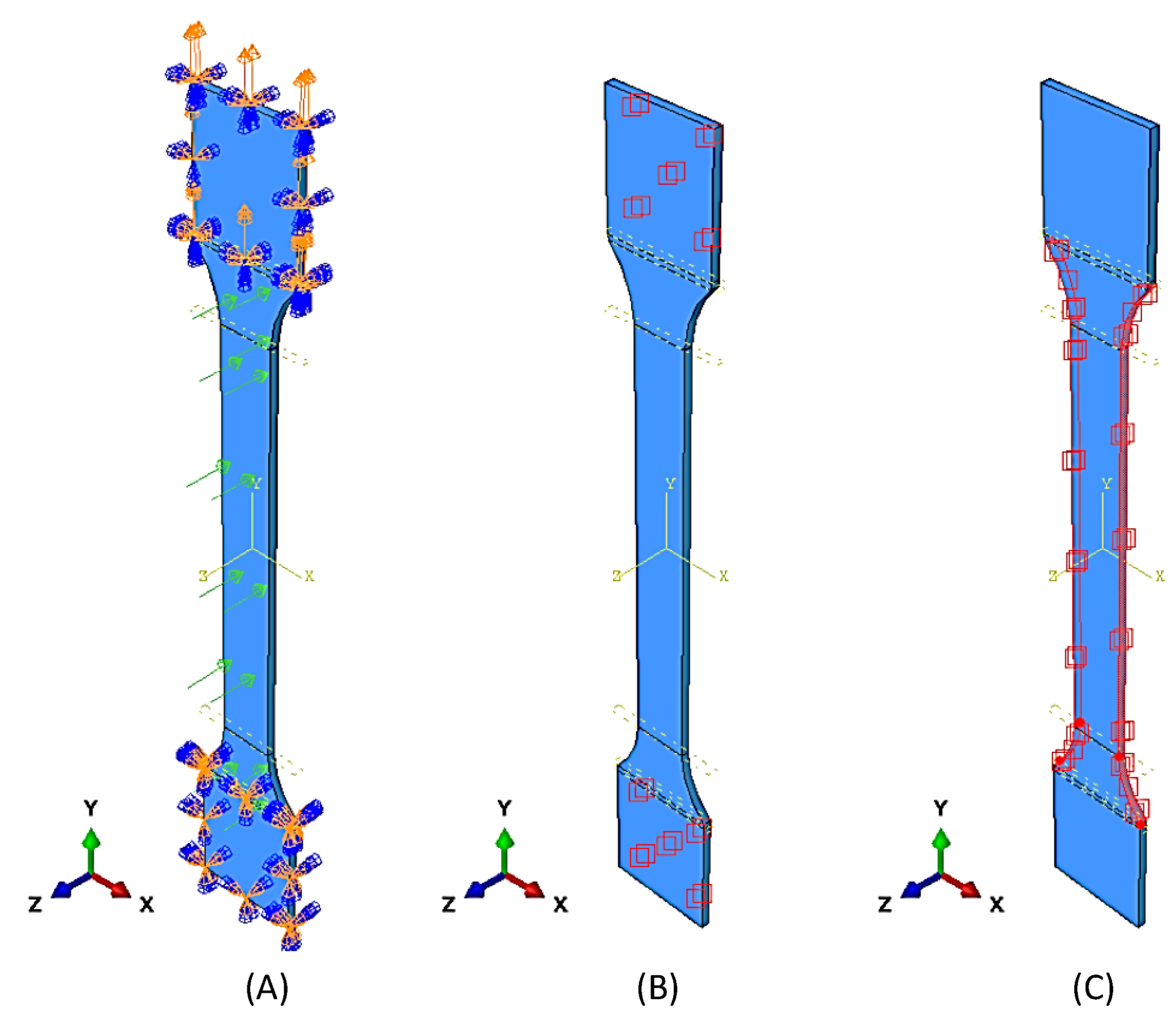
2.4.5. Concept for Thermomechanic FE-Analysis

The presented thermomechanical material model is transferred to the FE-software Abaqus 2022 for the three-dimensional case applying the user subroutine UMAT. In order to generate a realistic simulation, the geometry from Figure 1 was modelled. The coupled temperature displacement calculation is realised with eight-node thermally coupled, trilinear displacement and temperature elements (C3D8T). To realise the mechanical load, all displacements of the lower clamp are blocked, and the displacement of the upper clamp in the y-direction is released (Figure 6A, blue and orange arrows). As the experimental set-up includes the external radiator (Figure 2), it is considered in the FE-model (Figure 6A, green arrows). The effect of the radiator is analysed from the difference in the temperature evolution at the thermoelastic effect and the beginning of the holding times between the experiment and simulation. This influence is included in the model by a linear increase function with a final value of $r=0.065\mathrm{J}{\mathrm{s}}^{-1}{\mathrm{m}}^{-2}$. The convective interaction between the clamp areas and the machine jaws (Figure 2) is modelled with a surface film condition with the constant value $h=2.9\mathrm{J}{\mathrm{s}}^{-1}{\mathrm{m}}^{-2}{°\mathrm{C}}^{-1}$ [42] and a sink temperature ${\Theta }^s=20°\mathrm{C}$ (Figure 6B, red rectangles). Another boundary condition represents the convective interaction between the sample and the surrounding air. This condition is attached by a surface film condition on the outside of the sample with the constant value $h=2\mathrm{J}{\mathrm{s}}^{-1}{\mathrm{m}}^{-2}{°\mathrm{C}}^{-1}$ [42] and a sink temperature ${\Theta }^s=20°\mathrm{C}$ (Figure 6C, red marked area with red rectangles). The consideration of the air surface film is motivated by the differences in the temperature evolution of the experimental and the numerical curve during the second and the third holding time. As the film boundary condition through the clamping area did not remove enough heat from the system at these times, this additional boundary condition generated a more accurate result.

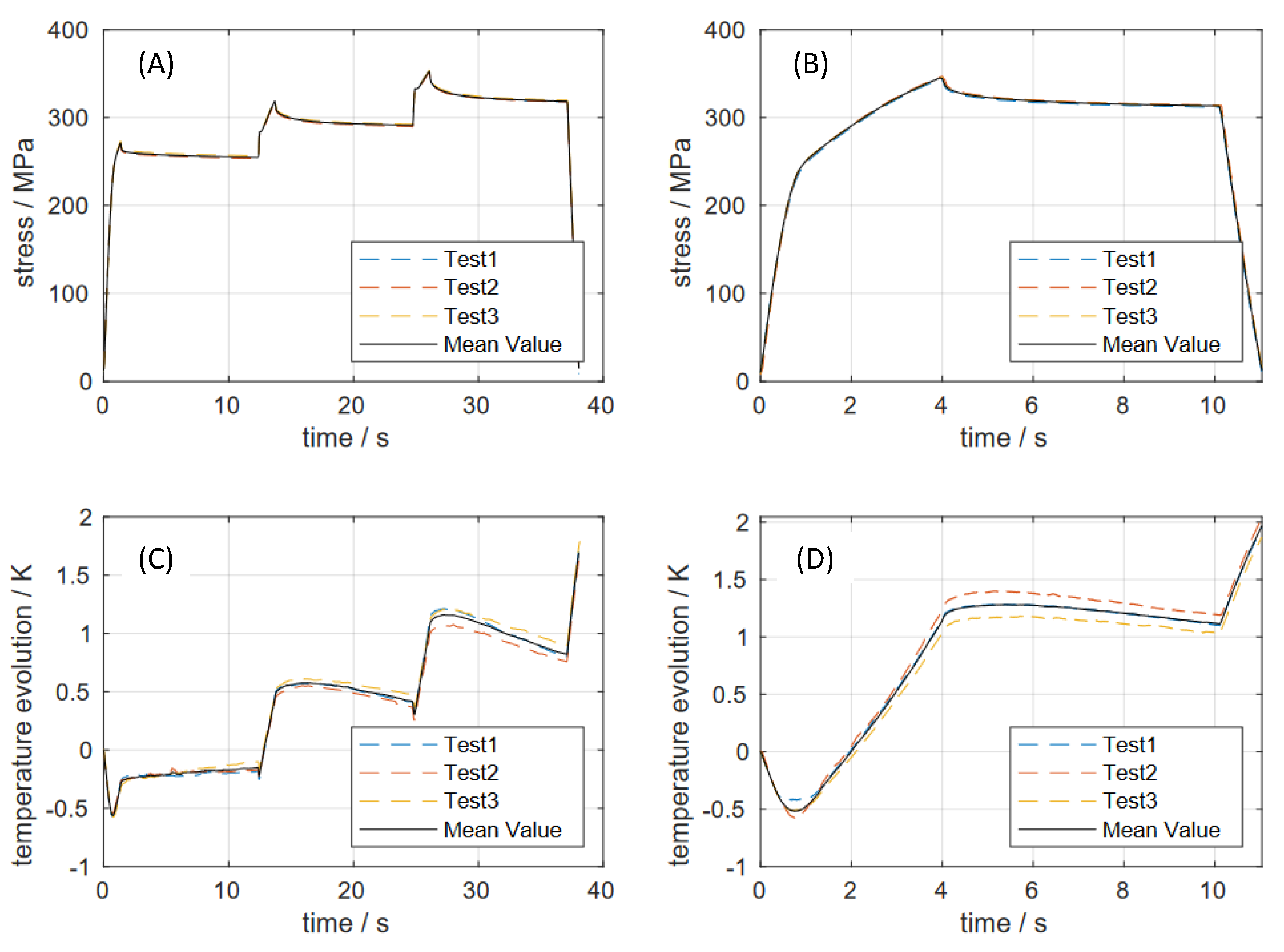
3. Results and Discussion

3.1. Parameter Determination

In order to determine the model parameters, some of them are estimated directly by the experimental curves ${\mathrm{v}}_1$. These include Young’s modulus E, the yield strength ${\sigma }^y$, and the Poisson value $\nu$. In particular, the elastic loading and unloading path (Figure 4) are helpful in the determination of Young’s modulus. Considering the microstructure analysis, the GTN parameters ${\widehat{f}}_0$ and ${\widehat{f}}^F$ are determined directly. The thermal parameters ${\alpha }^0$, $c^{\mathit{\sigma }}$ and k are based on the material’s data sheet [13]. For the experimental identification of the material’s mass density $\rho$, the weight of ten specimen is measured by the analytical balance ABJ220-4NM from the company Kern (Hamburg, Germany). With the volume of the samples, the mass density $\rho$ is calculated by the mass-to-volume ratio. Based on this direct identification method, the number of the unknown parameters decrease to six parameters for the elasto-viscoplastic material behaviour and to six parameters for the damage behaviour. All other parameters are identified using Matlab’s optimisation toolbox. The stress evolution and the temperature change in the sample surface are defined as objective functions with equal weighting. A MultiStart function based on creating random starting points in the parameter space and searching for a minima with the lsqnonlin algorithm [43] was chosen for parameter identification. The determined parameters for the description of the material behaviour are presented in

Table 2. Model parameters.

Symbol	Unit	Value	Symbol	Unit	Value	Symbol	Unit	Value
Chaboche  Parameters
$\nu$		0.34	E	MPa	47,998	${\sigma }^y$	MPa	213
K	MPa	1.4	n		4	${\mathrm{C}}^1$	MPa	1791
${\mathrm{C}}^2$	MPa	1432	${\gamma }^1$		56	${\gamma }^2$		5
$Q^{\infty }$		75	b		75	${\mathrm{R}}^{kin1}$	${\mathrm{s}}^{-1}$	0
${\mathrm{R}}^{kin2}$	${\mathrm{s}}^{-1}$	0	${\phi }_{\infty }^1$		0	${\phi }_{\infty }^2$		0
${\omega }^1$		0	${\omega }^2$		0
GTN  Parameters
${\widehat{f}}_0$		0.0373	$q_1$		1.3	$q_2$		1
${\widehat{f}}^F$		0.0385	${\widehat{f}}^N$		0.001	${\mathrm{s}}^N$		0.1
${\epsilon }^N$		0.3	${\widehat{f}}^C$		0.0382
Thermal  Parameters
$\rho$	g ${\mathrm{cm}}^{-3}$	2.66	${\alpha }^0$	${\mathrm{K}}^{-1}$	$2·{10}^{-5}$	$c^{\sigma }$	J ${\mathrm{kg}}^{-1}$ ${\mathrm{K}}^{-1}$	850
k	W ${\mathrm{m}}^{-1}$ ${\mathrm{K}}^{-1}$	150

.

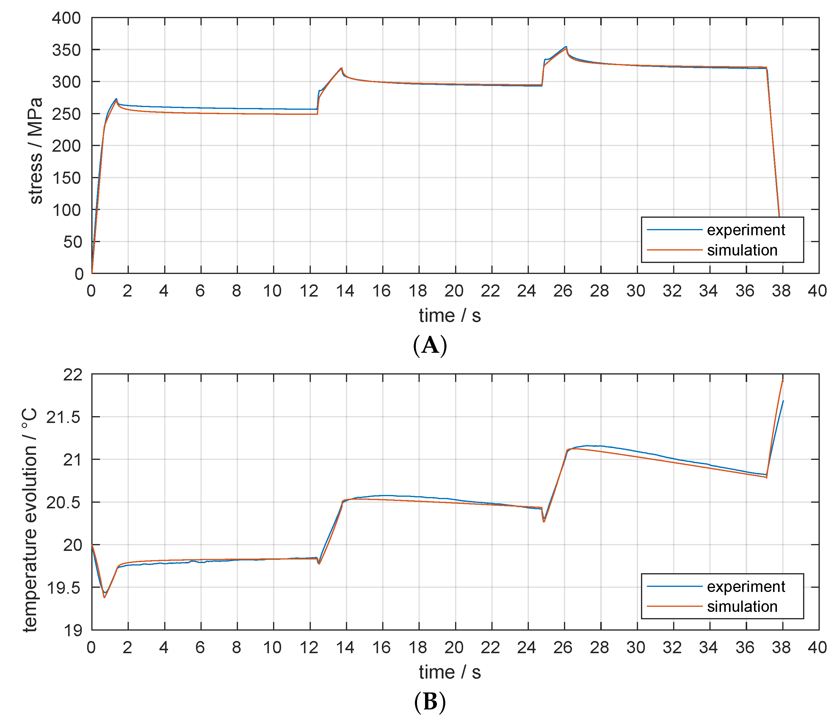
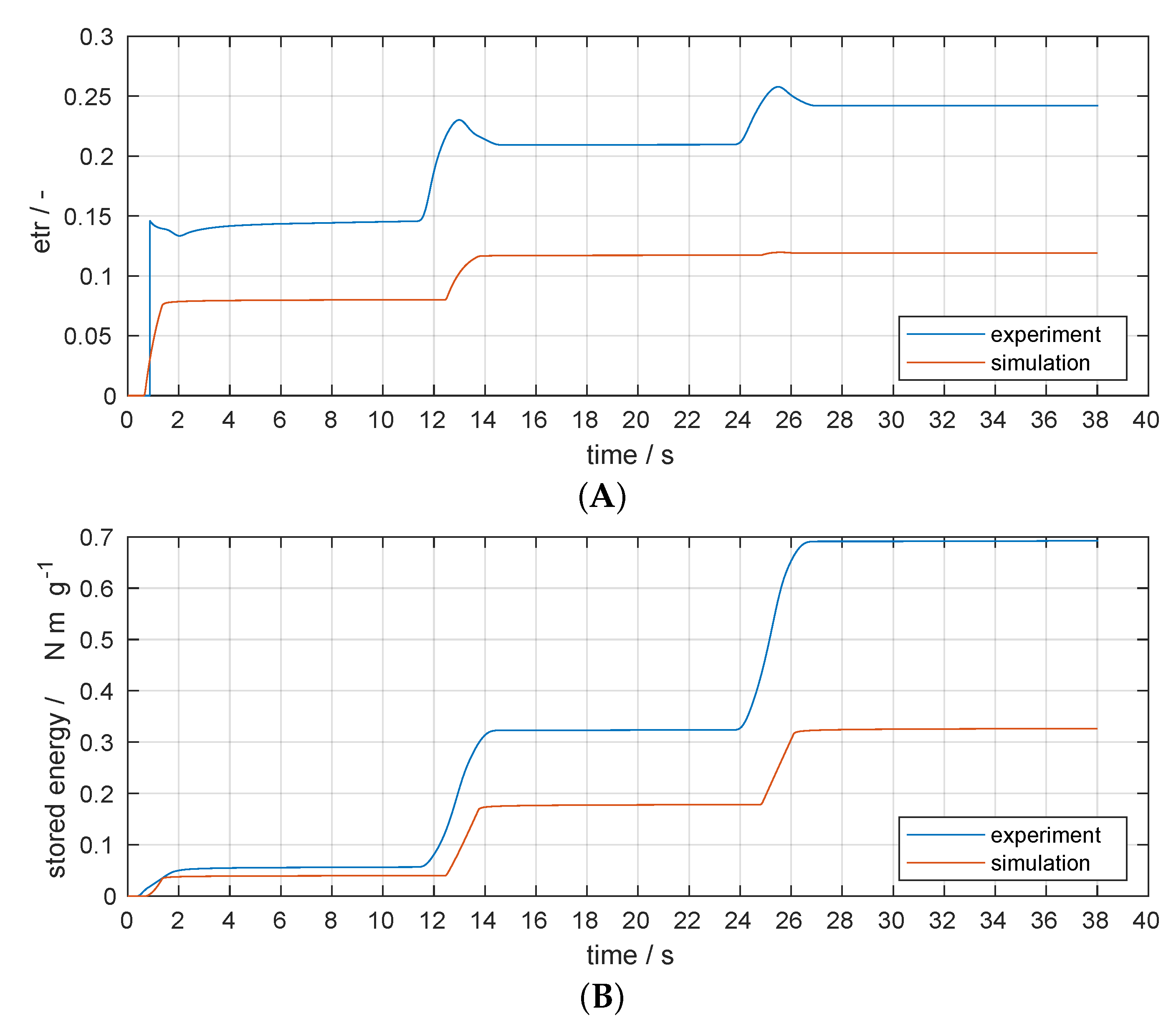
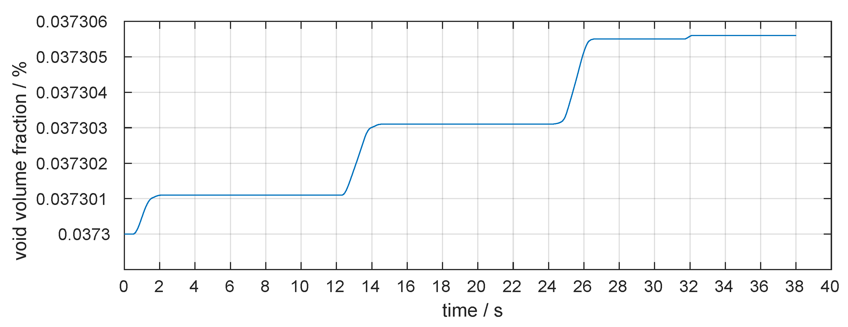
3.2. Numerical Results

Based on the determined parameters, numerical calculations were performed to verify the model. The experimental curves were generated in the centre of the sample; consequently, the region of interest is located in this area (Figure 7A, red dot). In the third load range after around 26 s (Figure 4), a plausibility check of the stress distribution (Figure 7B) and the temperature distribution (Figure 7C) was performed.

With respect to the boundary conditions of the system (Figure 6), an analysis of the thermomechanical response (Figure 7B,C) looks reasonable. In order to obtain a more detailed evaluation of the numerical model, its behaviour at the point (Figure 7A) is evaluated and compared with the experiments (Figure 8).

The identified material parameters of the selected model can represent the material behaviour with a high degree of accuracy. The highest difference in the stress behaviour of 10 MPa is located in the first holding time between 1 and 11 s. This error of 4% is in an acceptable range and the numerical simulation displays the main relaxation phenomena of the material. In the case of temperature characteristics, significant errors of max. $0.05$ K are present during the holding times. One reason for this error of 1% is the modelling of the thermal boundary conditions. To check these boundary conditions, the energy characteristics can be added to the analysis. To obtain the inelastic work $w^{vp}$, the area of the strain-hardening curve can be analysed based on the mechanical stress–strain characteristics. The dissipated heat is located by the self-heating phenomena. With this information, the stored energy $w^s$ is calculated as the difference in the inelastic work and the dissipated heat [44]. This additional information leads to the determination of the etr according to Equation (17).

Figure 9 illustrates the error between measured and simulated etr. This error is explained with the help of the stored energy evolution (Figure 9). The reason why there is a difference between the numerical simulation and experiment is that an adiabatic test was not performed. The radiator for the DIC (Figure 2) supplies the system with additional heat energy. This means that the experimentally determined curves show the stored energy, which is influenced by the radiator energy. Figure 9 demonstrates that the modelling of the radiator in the FE model is necessary. In addition, both energy distributions show that the dissipative character of the material is represented in an acceptable way.

As evidence of material damage, the void volume fraction ${\widehat{f}}^{*}$ evolution as a result of the void growing and void nucleation effects is presented in Figure 10. No void coalescence is considered because the void volume fraction ${\widehat{f}}^{*}$ is clearly below the coalescence criterion ${\widehat{f}}^c$. During elastic deformation, a constant void volume fraction is achieved at the initial porosity ${\widehat{f}}_0$. When the inelastic material behaviour begins, an increase in void volume fraction is observed until the start of the holding time at 1.4 s. A small non-linear increase in the void volume fraction follows at the beginning of the holding time, which can be linked to the initiation of relaxation in the stress behaviour (Figure 8). This phenomenon disappears after $0.5$ s and results in a constant void volume fraction value. The behaviour described is repeated until the end of the third holding time and looks plausible according to the rules of the GTN model (Equation (31)). With the unloading process at 32 s, a non-linear increase in void volume fraction is achieved. This phenomenon characterises the residual viscoplasticity, which is caused by the load reversal and reflected in the experimental stress evolution. An elastic behaviour of the material is achieved after the relaxation part, representing a reversible process. As a result of this reversibility, the microstructure is not changed, and the void volume fraction stays constant.

After the complex tensile test with multiple holding times ${\mathrm{v}}_1$ was extensively analysed, the simple tensile test with holding time ${\mathrm{v}}_2$ was intended to validate the identified material parameters. The differences in the etr characteristics do not depend on the selected material parameters; therefore, the stress and temperature characteristics in Figure 11 are sufficient for validation. Experiment v2 provides a more precise assessment of the material’s hardening behaviour than experiment v1. Test v2 is intended to also validate the ability to reproduce the hardening behaviour with the identified parameters. The comparison of the stress characteristics shows good agreement between the experiment and numerical simulation. The highest difference of 17 MPa is detected at the beginning of the holding time after 4 s. This corresponds to an acceptable relative error of 5%. The coupled field problem is clearly represented in the temperature characteristic. A small difference between the two curves is visible in the thermoelastic range up to 0.8 s, as already seen in the stress characteristics. Exceeding the yield point results in the beginning of highly dissipative inelastic deformations, characterised by the hardening and self-heating of the material. As the hardening in the simulation causes a higher stress at the start of the holding time, the calculated self-heating is also higher. Through this effect and the consideration of thermal boundary conditions, the calculated curve of the temperature characteristic exceeds the experiment. A clear deficit is given by the thermal behaviour during the holding time. The difference between the calculation and experiment is $0.24$ K and represents a relative error of $1.1$%. This phenomenon requires more detailed observation and consideration of the thermal boundary conditions.

4. Conclusions

This study demonstrates the thermomechanical enhancement of the Chaboche GTN model in representing the material stress and self-heating behaviour under complex loading scenarios. It is shown that the integration of the temperature characteristic into the parameter identification leads to a limited parameter determination and to a result with a high accuracy. The validation with the tensile test ${\mathrm{v}}_2$ supports this result. This paper demonstrates that the number of experiments for parameter identification can be reduced by a coupled analysis of the deformation and temperature field. For the next research steps, the experiment needs to be approximated to an adiabatic state. This concept can result in the integration of etr characteristics into the parameter identification process. In order to generate an nearly adiabatic process, a change in the measurement methodology as in [44] can be implemented. Additionally, the heat conduction effects can be minimised by significantly increasing the velocity as suggested in [45]. In case these modifications to the experimental set-up show a significant difference between the experimental and the calculated etr curve, the energetic approaches for the internal variables can be modified. An excellent study on this topic shows this difference [16]. The consideration of the void volume fraction shows an interesting initial effect at load reversal after inelastic material loading. This behaviour can be validated with the help of in situ tests and included in the parameter identification process. This study demonstrates access to the three-dimensional FE of the Chaboche-GTN model created in Abaqus. As a result, more complex geometry-related loading conditions can be analysed.

References

1. Bajaj, P.; Hariharan, A.; Kini, A.; Kürnsteiner, P.; Raabe, D.; Jägle, E.A. Steels in additive manufacturing: A review of their microstructure and properties. Mater. Sci. Eng. A 2020, 772, 138633–138658. [Google Scholar] [CrossRef]
2. Murr, L.E. Frontiers of 3D Printing/Additive Manufacturing: From Human Organs to Aircraft Fabrication. J. Mater. Sci. Technol. 2016, 10, 987–995. [Google Scholar] [CrossRef]
3. Goyanes, A.; Wang, J.; Buanz, A.; Martinez-Pacheco, R.; Telford, R.; Gaisford, S.; Basit, A.W. 3D Printing of Medicines: Engineering Novel Oral Devices with Unique Design and Drug Release Characteristics. Mol. Pharm. 2015, 11, 4077–4084. [Google Scholar] [CrossRef] [PubMed]
4. Asnafi, N.; Rajalampi, J.; Aspenberg, D.; Alveflo, A. Production Tools Made by Additive Manufacturing Through Laser-based Powder Bed Fusion. BHM Berg-Huettenmaennische Monatshefte 2020, 3, 125–136. [Google Scholar] [CrossRef]
5. Sun, C.; Wang, Y.; McMurtrey, M.D.; Jerred, N.D.; Liou, F.; Li, J. Additive manufacturing for energy: A review. Appl. Energy 2021, 282, 116041. [Google Scholar] [CrossRef]
6. Ngo, T.D.; Kashani, A.; Imbalzano, G.; Nguyen, K.T.Q.; Hui, D. Additive manufacturing 3D printing: A review of materials, methods, applications and challenges. Compos. Part B Eng. 2018, 143, 172–196. [Google Scholar] [CrossRef]
7. Sames, W.J.; List, F.A.; Pannala, S.; Dehoff, R.R.; Babu, S.S. The metallurgy and processing science of metal additive manufacturing. Int. Mater. Rev. 2016, 61, 315–360. [Google Scholar] [CrossRef]
8. Zhao, L.; Song, L.; Macías, J.G.S.; Zhu, Y.; Huang, M.; Simar, A.; Li, Z. Review on the correlation between microstructure and mechanical performance for laser powder bed fusion AlSi10Mg. Addit. Manuf. 2022, 56, 102914. [Google Scholar] [CrossRef]
9. Gruber, K.; Ziółkowski, G.; Pawlak, A.; Kurzynowski, T. Effect of stress relief and inherent strain based pre-deformation on the geometric accuracy of stator vanes additively manufactured from inconel 718 using laser powder bed fusion. Precis. Eng. 2022, 76, 360–376. [Google Scholar] [CrossRef]
10. Yadroitsev, I.; Yadroitsava, I.; Plessis, A.D. Fundamentals of Laser Powder Bed Fusion of Metals; Elsevier: Amsterdam, The Netherlands, 2021. [Google Scholar]
11. Calignano, F. Investigation of the accuracy and roughness in the laser powder bed fusion process. Virtual Phys. Prototyp. 2018, 13, 97–104. [Google Scholar] [CrossRef]
12. Pereira, J.C.; Gil, E.; Solaberrieta, L.; San Sebastián, M.; Bilboa, Y.; Rodríguez, P.P. Comparison of AlSi7Mg0.6 alloy obtained by selective laser melting and investment casting processes: Microstructure and mechanical properties in as-built/as-cast and heat-treated conditions. Mater. Sci. Eng. A 2020, 778, 139124. [Google Scholar] [CrossRef]
13. SLM Solutions. Available online: https://www.slm-solutions.com/fileadmin/Content/Powder/MDS/MDS_Al-Alloy_AlSi7Mg0_6_0219_EN.pdf (accessed on 28 June 2022).
14. Hesse, W. Aluminium Material Data Sheets; DIN Deutsches Institut für Normung e.V.: Berlin, Germany, 2016; pp. 268–271. [Google Scholar]
15. Richter, L.; Sparr, H.; Schob, D.; Maasch, P.; Roszak, R.; Ziegenhorn, M. Self-Heating Analysis with Respect to Holding Times of an Additive Manufactured Aluminium Alloy. In Proceedings of the IUTAM Creep in Structures VI, Magdeburg, Germany, 5 August 2023; Volume 16. [Google Scholar]
16. Broecker, C.; Matzenmiller, A. An enhanced concept of rheological models to represent nonlinear thermoviscoplasticity and its energy storage behavior. Contin. Mech. Thermodyn. 2013, 25, 749–778. [Google Scholar] [CrossRef]
17. Kamlah, M.; Haupt, P. On the macroscopic description of stored energy and self heating during plastic deformation. Int. J. Plast. 1998, 13, 893–911. [Google Scholar] [CrossRef]
18. Bodner, S.R.; Partom, Y. Constitutive Equations for Elastic-Viscoplastic Strain-Hardening Materials. J. Appl. Mech. 1975, 42, 385–389. [Google Scholar] [CrossRef]
19. Chaboche, J.L. Constitutive equations for cyclic plasticity and cyclic viscoplasticity. Int. J. Plast. 1989, 5, 247–302. [Google Scholar] [CrossRef]
20. Gurson, A.L. Continuum Theory of Ductile Rupture by Void Nucleation and Growth: Part I—Yield Criteria and Flow Rules for Porous Ductile Media. J. Eng. Mater. Technol. 1977, 99, 2–15. [Google Scholar] [CrossRef]
21. Chu, C.C.; Needleman, A. Void Nucleation Effects in Biaxially Stretched Sheets. J. Eng. Mater. Technol. 1980, 102, 249–256. [Google Scholar] [CrossRef]
22. Tvergaard, V.; Needleman, A. Analysis of the cup-cone fracture in a round tensile bar. Acta Metall. 1984, 32, 157–169. [Google Scholar] [CrossRef]
23. Schob, D.; Sagradov, I.; Roszak, R.; Sparr, H.; Franke, R.; Ziegenhorn, M.; Kupsch, A.; Léonard, F.; Müller, B.R.; Bruno, G. Experimental determination and numerical simulation of material and damage behaviour of 3D printed polyamide 12 under cyclic loading. Eng. Fract. Mech. 2020, 229, 106841. [Google Scholar] [CrossRef]
24. Schob, D. Experimentelle Untersuchung und Numerische Simulation des Material- und Schädigungsverhaltens von 3D Gedruckten Polyamid 12 unter Quasistatischer und Zyklischer Beanspruchung. Ph.D. Thesis, Brandenburgische Technische Universität, Cottbus, Germany, 2023. [Google Scholar]
25. Rose, L.; Menzel, A. Optimisation based material parameter identification using full field displacement and temperature measurements. Mech. Mater. 2020, 145, 103292. [Google Scholar] [CrossRef]
26. Song, P.; Trivedi, A.; Siviour, C.R. Tensile testing of polymers: Integration of digital image correlation, infrared thermography and finite element modelling. J. Mech. Phys. Solids 2023, 171, 105161. [Google Scholar] [CrossRef]
27. Haupt, P. Continuum Mechanics and Theory of Materials, 2nd ed.; Springer: Berlin/Heidelberg, Germany, 2002. [Google Scholar]
28. Truesdell, C.; Noll, W. The Non-Linear Field Theories of Mechanics, 3rd ed.; Springer: Berlin, Germany, 1992. [Google Scholar]
29. Gurtin, M.E.; Fried, E.; Anand, L. The Mechanics and Thermodynamics of Continua; Cambridge University Press: Cambridge, UK, 2013. [Google Scholar]
30. Coleman, B.D.; Gurtin, M.E. Thermodynamics with internal state variables. J. Chem. Phys. 1967, 47, 597–613. [Google Scholar] [CrossRef]
31. Bever, M.; Holt, D.; Titchener, A. The stored energy of cold work. Prog. Mater. Sci. 1973, 17, 5–177. [Google Scholar] [CrossRef]
32. Rosakis, P.; Ravichandran, G.; Hodowany, J. A thermodynamic internal variable model for the partition of plastic work into heat and stored energy in metals. J. Mech. Phys. Solids 2000, 48, 581–607. [Google Scholar] [CrossRef]
33. Egner, W.; Egner, H. Thermo-mechanical coupling in constitutive modeling of dissipative materials. Int. J. Solids Struct. 2016, 91, 78–88. [Google Scholar] [CrossRef]
34. Sparr, H. Thermomechanische Analyse von Inelastischen Deformationsvorgaengen bei Komplexer Beanspruchung in Modellierung und Experiment. Ph.D. Thesis, Brandenburgische Technische Universität, Cottbus, Germany, 2023. [Google Scholar]
35. Smolina, I.; Gruber, K.; Pawlak, A.; Ziółkowski, G.; Grochowska, E.; Schob, D.; Kobiela, K.; Roszak, R.; Ziegenhorn, M.; Kurzynowski, T. Influence of the AlSi7Mg0.6 Aluminium Alloy Powder Reuse on the Quality and Mechanical Properties of LPBF Samples. Materials 2022, 15, 5019. [Google Scholar] [CrossRef] [PubMed]
36. Goettfert, F.; Sparr, H.; Ziegenhorn, M.; Dammass, G.; Krauß, M. Combining thermography and stress analysis for tensile testing in a single sensor. SPIE 2022, 12109, 121090A. [Google Scholar]
37. ASTM E328-20; Standard Test Methods for Stress Relaxation for Materials and Structures. ASTM: West Conshohocken, PA, USA, 2021. Available online: https://cdn.standards.iteh.ai/samples/108269/b1b76a85ade941c6b284b4db71cb46ba/ASTM-E328-20.pdf (accessed on 23 July 2024).
38. Kamlah, M. Zur Modellierung des Verfestigungsverhaltens von Materialien mit Statischer Hysterese im Rahmen der Phaenomenologischen Thermomechanik. Ph.D. Thesis, Universität Gesamthochschule, Kassel, Germany, 1994. [Google Scholar]
39. Coleman, B.D.; Noll, W. The Thermodynamics of Elastic Materials with Heat Conduction and Viscosity. Arch. Ration. Mech. Anal. 1963, 13, 167–178. [Google Scholar] [CrossRef]
40. El Khatib, O.; Hütter, G.; Pham, R.D.; Seupel, A.; Kuna, M.; Kiefer, B. A non-iterative parameter identification procedure for the non-local gurson-tvergaard-needleman model based on standardized experiments. Int. J. Fract. 2023, 241, 73–94. [Google Scholar] [CrossRef]
41. Chaboche, J.L. Cyclic Viscoplastic Constitutive Equations, Part I: A Thermodynamically Consistent Formulation. J. Appl. Mech. 1993, 60, 813–821. [Google Scholar] [CrossRef]
42. Cengel, Y.A. Heat Transfer: A Practiacal Approach; McGraw Hill: New York, NY, USA, 2016. [Google Scholar]
43. Matlab. Available online: https://de.mathworks.com/help/gads/patternsearch.html (accessed on 11 December 2023).
44. Oliferuk, W.; Raniecki, B. Thermodynamic description of the plastic work partition into stored energy and heat during deformation of polycrystalline materials. Eur. J. Mech.-A/Solids 2018, 71, 326–334. [Google Scholar] [CrossRef]
45. Golasinski, K.M.; Staszczak, M.; Pieczyska, E.A. Energy Storage and Dissipation in Consecutive Tensile Load-Unload Cycles of Gum Metal. Materials 2023, 16, 3288. [Google Scholar] [CrossRef] [PubMed]
Figure 1. (A) Sample orientation during the manufacturing process (B) Sample geometry.
Applmech 05 00030 g001
Figure 2. Concept of a thermomechanical experimental set-up.
Applmech 05 00030 g002
Figure 3. User interface of the post−processing tool.
Applmech 05 00030 g003
Figure 4. Input strain path. v 1 : complex load path with multiple holding times and an unloading step. v 2 : tension test with one holing time and an unloading step.
Applmech 05 00030 g004
Figure 5. Results of the thermomechanical experiments: (A) the material’s stress response for the strain rate v 1 ; (B) the material’s stress response for the strain rate v 2 ; (C) the material’s temperature response for the strain rate v 1 ; (D) the material’s temperature response for the strain rate v 2 .
Applmech 05 00030 g005
Figure 6. Boundary conditions: (A) displacement boundary conditions and radiator, (B) surface film condition on clamped area, and (C) surface film condition for air convection.
Applmech 05 00030 g006
Figure 7. FE−Results at t = 26 s: (A) region of interest, (B) stress distribution in the y-direction, and (C) temperature distribution.
Applmech 05 00030 g007
Figure 8. Thermomechanical material behaviour for loading path v 1 (A) Mechanical behaviour (B) Temperature behaviour.
Applmech 05 00030 g008
Figure 9. Energy behaviour for loading path v 1 (A) Energy transformation ratio (B) Stored energy of cold work.
Applmech 05 00030 g009
Figure 10. Numerical void volume fraction f ^ * for loading path v 1 .
Applmech 05 00030 g010
Figure 11. Thermomechanical material behaviour for the loading path v 2 (A) Mechanical behaviour (B) Temperature behaviour.
Applmech 05 00030 g011