Enhancing Spreading Factor Assignment in LoRaWAN with a Geometric Distribution Approach for Practical Node Distributions

Abstract

This paper proposes the GD (Geometric Distribution) algorithm, a novel approach to enhance the default Adaptive Data Rate (ADR) mechanism in the Long-Range Wide Area Network (LoRaWAN). By leveraging the Probability Mass Function (PMF) of the GD model, the algorithm effectively addresses biased node distributions encountered in real-world scenarios. Its ability to finely adjust the weight factor (w) or the probability of success in allocating SFs enables the optimization of spreading factor (SF) allocation, thereby achieving the optimal Data Extraction Rate (DER). To evaluate the algorithm’s performance, simulations were conducted using the fixed node pattern derived from actual dairy farm locations in Ratchaburi province, Thailand. Comparative analyses were performed against the uniform random node pattern and existing algorithms, including the ADR, EXPLoRa, QCVM, and SD. The GD algorithm significantly outperformed existing methodologies for both fixed and uniform random node patterns, achieving a 14.3% and 4.8% improvement in DER over the ADR, respectively. While the GD algorithm consistently demonstrated superior DER values across varying coverage areas and payload sizes, it incurred a slight increase in energy consumption due to node allocations to higher SFs. Therefore, the trade-off between DER and energy consumption must be carefully weighed against the specific application.

1. Introduction

Low-Power Wide Area Network (LPWAN) [1] has now emerged as one of the most popular wireless networks for the Internet of Things (IoT). LPWAN has found various applications in areas such as smart cities, smart logistics, and smart farming. Long-Range Wide Area Network (LoRaWAN) [2] is one of the LPWAN technologies that has received much attention for the past several years due to its low power consumption, large coverage area, high security, long battery life, and low cost. Compared with proprietary LPWAN technologies such as NB-IoT [3] and Sigfox [4], the non-proprietary LoRaWAN opens the door for individual users to adopt, build, learn, and research the technology freely.

LoRaWAN uses the chirp spread spectrum (CSS) as a signal modulation technique in the physical layer. The packet and propagation characteristics are classified into groups of spreading factors (SFs) that are determined based on the received signal strength indicator (RSSI) and propagation distance of each packet. The typical values of SF are 7–12. The smaller SF offers higher data rate and shorter time-on-air (ToA) while the larger SF offers lower data rate and longer ToA. LoRaWAN adopts the pure ALOHA protocol, which allows simultaneous packet transmission by multiple end devices or nodes over a common radio channel; therefore, it inevitably suffers from packet loss due to collision. Note that a packet collision is confirmed when two or more colliding packets have the same SF value and frequency, or the same chirp rate. To alleviate the problem, altering the data rate and, thus, the ToA of end devices or SF allocation, is a widely used approach.

Various pieces of research focused on the applications of LoRaWAN. Examples include deploying gas sensors to remotely collect data for air pollution control [5] and the integration of LoRaWaN to the smart water resource management equipped with measurement systems of water availability, soil moisture, topography, and plant identification [6,7]. They found that LoRaWAN could improve the data transmission and, thus, the data extraction rate (DER), which is the ratio between the data packets successfully sent and all data packets in a defined period.

Other previous research explored and improved LoRaWAN performance in different environments. The LoRaWAN network infrastructure was implemented for a universal sensor, where it was proved to consume lower energy and operated well under real-life conditions [8]. The LoRaWAN performance with mobile nodes was evaluated in an urban environment and was found to provide shorter data transmission range than in open environments [9]. The path-loss propagation model for LoRaWAN was then optimized in certain environments to ensure the positive results [10].

A default mechanism used for optimizing the data rate, ToA, and energy consumption of an end device or node in LoRaWAN is the adaptive data rate (ADR) [11]. The ADR optimizes these parameters by considering RSSI and link budget. When multiple nodes are placed in a confined area, their RSSI values are nearly the same, as are their SF values. Although the ADR is activated, the SF values are not sufficiently distributed; thus, the co-SF interference or packet collision due to similar SF still occurs. Note that co-SF interference occurs when multiple nodes transmit simultaneously on the same channel using the same spreading factor (SF), leading to overlapping signals. Therefore, several previous works aimed to improve the network performance, reducing the co-SF interference by better SF allocation or assignment. While previous studies have demonstrated the potential for inter-SF interference between different SFs, decoding LoRa signals with the co-SF interference is significantly challenging [12]. For simplicity, we assume negligible inter-SF interference in our analysis.

We have summarized six schemes for improving SF allocation that include SNR-based, RSSI-based, ToA-based, distance-based, machine learning (ML), and descriptive statistic schemes.

The SNR-based SF scheme focuses on SF assignment based on the target Signal-to-Noise Ratio (SNR) of the received packet and the impact of channel fading and distance [13]. The Best-Equal LoRa (BE-LoRa) algorithm was proposed to improve the packet delivery ratio (PDR) through the optimization and balancing of the SINR of received packets at the gateway for proper power setting and SF updates [14].

The RSSI-based and ToA-based schemes were designed to mitigate the co-SF interference during message transmission, thereby enhancing overall network efficiency and reliability. For instance, the EXPLoRa-SF algorithm compared the RSSI values with the sensitivity levels and divided them into six SF groups with equal numbers of nodes to create coexisting orthogonal sub-channels in the same channel bandwidth [15]. The authors also proposed the EXPLoRa-AT algorithm to balance the total offered packets (load) by utilizing the ordered waterfilling of SFs that then guaranteed the ToA equalization in each SF group. In [16], the authors proposed EXPLoRA-C, where the ordering of RSSI values and ToA-based techniques were combined using the concept of “sequential waterfilling” to assign the SF until the total offered packets in each SF group was full.

The distance-based scheme involves assigning SFs to nodes based on their distances from the gateway. Examples include equal-interval-based (EIB) and equal-area-based (EAB) SF allocation methods [12]. In the EIB and EAB schemes, the network area was divided into concentric circles of equal intervals and equal areas, respectively. In the EIB scheme, lower SFs are assigned to nodes in inner annuli, which are closer to the gateway, resulting in higher packet success probability in interference-prone environments. Conversely, the EAB scheme improves packet success probability at longer distances by mitigating near–far effects in smaller outer annuli.

In [17] and [18], the ML-based schemes were reported. In [17], the LR-RL method based on reinforcement learning (RL) for SF channel allocation in one-hop and in the LoRa mesh network was proposed. The method optimized the SF value based on channel traffic equilibrium by providing positive rewards for successful packet delivery and negative rewards otherwise. Consequently, the optimal SF value that minimizes SF collision rates was determined. In addition, [18] proposed a rapid, converging, decentralized RL algorithm for SF allocation aimed at maximizing packet reception ratio.

Apart from the abovementioned schemes, the descriptive statistics approach has become another promising scheme to improve SF allocation due to its simplicity. In [19], the researchers proposed the Quantile Classification of Variance from the Mean (QCVM) method that uses the statistical method, namely, the quantile classification to group RSSI data considering their mean and probability density function (PDF). Then, they proposed the Standard Deviation (SD) classification method that analyzed RSSI data of nodes before separating them into groups by the standard deviation (SD) and re-assigning the SF values in each group [20]. Both descriptive statistics-based approaches were, however, constrained by the fixed number of SF subclasses allowed within each SF group.

It is known that most SF allocation algorithm developments begin with simulations prior to the actual implementations. The node locations are commonly generated in the uniform random distribution, which is the default setting in most LoRaWAN simulators. However, the real-life node patterns often exhibit non-uniform or biased node distributions; thus, the uniform random distribution does not always give accurate insights in real-world scenarios [21,22,23] and potentially compromises the efficacy of prior algorithms in such contexts.

This research introduces the Geometric Distribution (GD) algorithm, a novel inferential statistics approach that leverages the Probability Mass Function (PMF) of the geometric distribution mathematical model [24] to address the challenge of non-uniform or biased SF node distribution. By incorporating this framework, the GD algorithm aims to enhance the default Adaptive Data Rate (ADR) mechanism in the LoRaWAN. The key of the GD algorithm is to identify the optimal distribution format for the intensive SF values by assigning weights or the probabilities of success for SF allocation to each SF category. The workflow begins by grouping nodes based on their RSSI levels, followed by the assignment of a defined SF value to nodes in each group. The most biased SF group is ingested into the GD algorithm. Within this algorithm, the biased SFs are reassigned to higher SF values through finely tuning the weight factor (w) via an intricately linked geometric distribution factor (p-value). This iterative process continues until the optimal p-value and corresponding weight factor (w) that yields the highest DER of the network are identified. In fact, we also considered developing the algorithm based on binomial and negative binomial distributions. Unlike the GD, both distributions were not directly developed to optimize the probability of success for SF allocation in the biased node environment.

Beyond its flexibility in finely tuning the weight factor to attain the optimal DER, the GD algorithm also exhibits algorithmic simplicity that allows ease of development and implementation. Similar to SNR-based and RSSI-based SF allocation schemes, the GD algorithm workflow leverages RSSI data measured by the gateway (see Section 5). This allows for direct integration with LoRaWAN and enables dynamic adaptation to various scenarios. The workflow can be structured to run the algorithm iteratively, to continuously update the SFs. For instance, RSSI levels of nodes can be regularly updated to enable re-grouping before the next iteration.

The summary of SF allocation schemes and contributions are summarized in

Table 1. Summary of SF allocation schemes and contributions.

SF Allocation Scheme	Approach and References	Publication Year	Contribution
ADR	Adaptive data rate [11]	2019	The ADR scheme is a default mechanism of LoRaWAN that allows the network to dynamically adjust the data rate and spreading factor (SF) of a device’s transmission based on its signal quality and network load.
SNR-based SFs	SNR-based allocation [13]	2021	This paper introduced an SF allocation scheme based on the target Signal-to-Noise Ratio (SNR) of the received packet and the impact of channel fading and distance.
	Best-Equal LoRa (BE-LoRa) [14]	2022	This paper introduced an SF allocation scheme through the optimization and balancing of the SINR of received packets at the gateway for proper power setting and SF updates.
RSSI-based SFs	EXPLoRa-SF [15]	2017	This paper introduced a SF allocation scheme where SFs were distributed equally to the nodes based on their RSSI values to create coexisting orthogonal sub-channels in the same channel bandwidth, enabling simultaneous communication among all nodes.
Time-on-Air-based SFs	EXPLoRa-AT [15]	2017	This paper introduced an SF allocation scheme by balancing the total offered packets (load) through the ordered waterfilling of SFs that then guaranteed the ToA equalization in each SF group.
	EXPLoRa-C [16]	2021	This paper introduced an SF allocation scheme by demonstrating a concept of sequential waterfilling, where nodes were firstly ordered based on their RSSI values and then were allocated to the given SF group until the total offered packets in the group is full.
Distance-based SFs	EIB and EAB [12]	2018	This paper proposed two SF allocation schemes: EIB, which divides the network area into concentric circles of equal intervals, and EAB, which uses equal areas. In the EIB scheme, lower SFs are assigned to inner annuli, resulting in higher packet success probability in interference-prone environments. Conversely, the EAB scheme improves packet success probability at longer distances by mitigating near–far effects in smaller outer annuli.
Machine learning-based SFs		2023	This paper proposed the LR-RL algorithm, which is a reinforcement learning algorithm designed to optimize SF allocation based on channel traffic equilibrium, aiming at mitigating packet collisions. Nodes will receive positive rewards for successful packet delivery and negative rewards otherwise.
	LR-RL [17] Decentralized reinforcement learning [18]	2023	This paper proposed the SF allocation scheme by treating the SF allocation as a contextual multi-arm bandit problem, which was solved for packet reception ratio (PRR) maximization using the decentralized EXP4 reinforcement learning algorithm that can converge quickly.
Descriptive Statistics-based SFs	Quantile classification of the variance from the mean [19]	2021	This paper introduced an SF allocation scheme where the quantile classification was applied to assign new SFs based on the mean and probability density function (PDF) of the RSSI data in each original SF group.
	Standard deviation classification [20]	2021	This paper introduced an SF allocation scheme where the standard deviation was applied to assign new SFs based on the mean and standard deviation of the RSSI data inside each original SF group.
This paper	Geometric Distribution (GD)	2024	This paper introduces an SF allocation scheme by using the Geometric Distribution (GD) algorithm, a novel inferential statistics approach to address the challenge of non-uniform or biased SF node distribution. The algorithm possesses flexibility in finely tuning the weight factor (w) via an intricately linked geometric distribution factor (p-value) until the optimal p-value and corresponding weight factor (w) that yields the highest DER of the network are identified.

.

The comparison between abovementioned SF allocation schemes was performed over the three following features:

• Performance: indication of the overall system throughput.
• Ease of implementation (complexity): indication of the amount of processing resource required at the gateway to decode a transmitted packet from a node.
• Application: indication of ability to handle dynamic scale of the network such as scenario mitigation, number of nodes, and inclusion and exclusion of nodes.

Results are shown in

Table 2. Comparison of SF allocation schemes with various features.

SF Allocation Scheme	Type	Performance	Ease of Implementation (Complexity)	Application	References
ADR	Dynamic	High	High	Yes	[11,25]
SNR-based SFs	Dynamic	High	High	Yes	[13,14,25]
RSSI-based SFs	Dynamic	Moderate	Moderate	Yes	[15,16]
Time-on-Air-based SFs	Dynamic	High	Moderate	Yes	[15,16]
Distance-based SFs	Static	Moderate	Moderate	No	[12,25]
Machine learning-based SFs	Dynamic	High	High	Yes	[17,18,25]
Descriptive Statistics-based SFs	Dynamic	QCVM—Moderate SD–High	Moderate	Yes	[19,20]
The proposed GD algorithm	Dynamic	High	Moderate	Yes	This paper

.

While these mentioned SF allocation schemes often enhance network throughput, they typically require increased energy consumption. To achieve a balance between throughput and energy consumption, several strategies can be considered. Dynamic SF allocation schemes, which can adjust SFs based on current network conditions, are generally preferable to static schemes. Additionally, implementing power-saving modes and adaptive transmission power can help conserve energy. Furthermore, clustering nodes and allocating SFs within each cluster based on individual node requirements can improve overall energy efficiency. However, when making trade-offs, the specific needs of the application must be carefully considered.

Our research applied the proposed GD algorithm to the LoRaWAN simulations conducted using the LoRaSIM simulator, a widely known Python-based LoRaWAN simulator developed by Thiemo Voigt and Martin Bor from University of Lancaster in UK. To assess the impact of node distribution on network performance, a comparative analysis was undertaken. This analysis compared results obtained from the uniform random node distribution scenario to those obtained from the fixed node distribution assumed based on the locations of dairy farms around the Photharam district, Ratchaburi province, Thailand [23]. This particular site was selected because it plans to implement Internet of Things (IoT) sensors to collect behavior data from dairy cows. The novelty of our algorithm lies in its ability to work effectively with biased node distributions and still achieve high DER values by finely tuning the weight factor. This adaptability ensures the algorithm’s efficacy across various scenarios, which provides valuable insights for improving network performance under diverse conditions.

The paper is divided into subsections as follows. Section 2 provides a brief overview of LoRaWAN. Section 3 delves into the comparison of fixed and random node simulation, while Section 4 and Section 5 expound on the geometric distribution mathematical model and the proposed algorithm, respectively. Section 6 covers the details of the experimental simulation, and the discussion and analysis of results are presented in Section 7. The research concludes with a summarizing section outlining the key findings and implications of the study.

2. LoRaWAN Overview

LoRa is a protocol in the physical layer of an IoT network. This protocol operates in the industrial, scientific, and medical radio bands (ISM band), or 902–928 MHz in Thailand. The LoRa protocol can endure the noise floor and interference by Chirp spread spectrum (CSS) techniques. The highlighted advantages are low power consumption and long-range coverage area. The characteristics of the CSS modulation depend on the LoRa’s parameters such as bandwidth (BW), SF, Coding Rate (CR), and the airtime defined in terms of the symbol period (T_S) shown in Equation (1). The bit rate (R_b) is related to BW, SF, and CR, as shown in Equation (2).

$$T_s={\displaystyle \frac{2^{SF}}{BW}},$$

(1)

$$R_b=SF\times {\displaystyle \frac{BW}{2^{SF}}}\times CR,$$

(2)

LoRaWAN is a network architecture consisting of end devices or nodes that employ the LoRa protocol for transmitting and receiving packets as well as the LoRa gateway, network server, and application server. In LoRaWAN, we can define the data rate, time-on-air (ToA), and signal range by assigning the SF values, which are the unique parameters in LoRa modulation, as shown in Figure 1.

LoRaWAN utilizes the Adaptive Data Rate (ADR), which is a default mechanism for optimizing the data rate, airtime, distance, and energy consumption when the signal strength varies dynamically, for example, in the case of dense and moving nodes. The link budget is the RSSI sensitivity level, which depends on the Signal-to-Noise Ratio (SNR), Noise Figure of receiver (NF), and bandwidth (BW). The link budget is presented in terms of the sensitivity value (S) shown in Equation (3). The SNR limit is dependent on the end device, and the NF of a typical LoRa gateway chipset is 7 dB [11]. The sensitivity level is also displayed in Figure 1.

$$S=-174+10\mathit{log}BW+NF+SN{R}_{lim},$$

(3)

Time-on-air (ToA) refers to the amount of time a device spends transmitting a packet. It is a crucial metric that directly impacts network performance and energy consumption. In a network with nodes and a single gateway, ToA can be considered synonymous with latency. ToA can be calculated using Equation (4).

$$ToA=T_{preamble}+T_{payload}$$

(4)

where

T_preamble is the preamble duration (in second);

T_payload is the payload duration (in second);

T_payload is directly proportional to the number of payload symbols (n_payload), which can be calculated as

$$n_{payload}=8+max\left[Ceil\left({\displaystyle \frac{8PL-4SF+28+16CRC-20H}{4\left(SF-2DE\right)}}\right)\times \left(CR+4\right),0\right],$$

(5)

where

PL = Payload Length (in Bytes);

H = the explicit header (H = 0 when enabled, = 1 when not);

CRC = the Cyclic Redundancy Check (CRC = 1 when enabled, = 0 when not);

CR = Coding Rate (CR = 1, 2, 3, 4);

DE = Low Data Rate Optimization (DE = 1 when used, = 0 when not).

It can be deduced from Equations (4) and (5) that ToA is indeed a function of SF value and also increases with the SF value, as illustrated in Figure 1.

Equation (6) demonstrates the direct correlation between the total ToA and total energy consumption (E) (in joules) across all S identical nodes, indicating that higher SF values lead to increased energy consumption. Note that the transmission current as well as the supplied voltage to the node are assumed equal for all nodes.

$$E=\sum _{n=1}^S({ToA}_n\times I\times V),$$

(6)

where

ToA_n is the ToA of the successfully sent nth node (in seconds);

I is the transmission current of the node (in A);

V is the supplied voltage to the node (3 V) [2].

3. Network Simulations for Fixed and Uniform Random Patterns of Nodes

The network simulation is an important approach to better anticipate the results of the actual network performance. It also sheds some light on what the network performance would be like in case the actual implementation cannot take place. However, most previous simulation works relied on generating a uniform random node pattern that could significantly deviate from the real-world scenario. This section aims at understanding the effect of node patterns on SF assignment and network performance by comparing fixed and random node patterns using the default ADR scheme.

Before constructing the node pattern, the propagation path loss model suitable for the study area was selected for the simulation. In our investigation, we conducted a survey at a considerable number of dairy farms in the Photharam district of Ratchaburi, Thailand. This area has the potential to adopt smart livestock technologies, and some farms have already pursued such technologies. We installed the LoRa gateway at Centermilk Farm and then conducted several drive tests in a 5 km radius, as shown in Figure 2, to measure the LoRa signal strength before creating a map to locate dairy farms within the test area. Photharam district is situated outside urban areas, characterized by small buildings and villages. Although present, these structures are not as numerous or densely populated as in urban areas. Thus, this environment aligns better with the suburban Hata–Okumura path loss model [26], as indicated by Equations (7)–(11). For simplicity, the path loss equation is shortened by using the variables A, B, and C to represent its three components. Note that the choice of path loss model depends on several factors such as environment type, operating frequency, communication range, propagation conditions, etc.

$$L_c=A+B\mathit{log}(d)-a(h_m)+C,$$

(7)

$$A=69.55+26.16\mathit{log}(f)-13.82\mathit{log}(h_b),$$

(8)

$$B=44.9-6.55\mathit{log}(h_b),$$

(9)

$$a\left(h_m\right)=\left(1.1\mathit{log}(f\right)-0.7)h_m-(1.56\mathit{log}(f)-0.8),$$

(10)

$$C=-2\left(\mathit{log}({\displaystyle \frac{f}{28}}\right){)}^2-5.4,$$

(11)

where

L_c is the total path loss (in dB);

d is the distance of end devices (in meters);

h_m is the height of end devices (in meters);

f is the frequency (in Kilohertz);

h_b is the height of the gateway (in meters);

a(h_m) is the correction factor for suburban environment (in dB).

Figure 2. Location of dairy farms at Photharam district, Ratchaburi, Thailand.

Figure 2. Location of dairy farms at Photharam district, Ratchaburi, Thailand.

In our research, we assigned 1500 nodes to represent 1500 connected dairy cows raised on the dairy farms in Photharam district, Ratchaburi. Note that the connected dairy cows are those tagged with the IoT sensors. We introduced node positions in the 2D plane with x and y coordinates, as expressed in Equations (12) and (13). Subsequently, we calculated the distance D from the node to a gateway using the Pythagorean formula, as shown in Equation (14).

$$x=K\times D_{max}\cos \left({\displaystyle \frac{I}{J}}\right),$$

(12)

$$y=K\times D_{max} \mathrm{s}\mathrm{i}\mathrm{n}\left({\displaystyle \frac{I}{J}}\right),$$

(13)

$$D=\sqrt{x^2+y^2},$$

(14)

where

D_max is the coverage area in meters;

x and y are the positions in the 2-dimensional plane;

D is the distance between the node and the gateway in meters;

I, J, and K are values between 0 and 1.

First, we utilized the LoRaSim simulator to randomize I, J, and K constants to generate the uniform random node pattern, as shown in Figure 3. Then, we assigned certain values of I, J, and K constants using Equations (12)–(14) to reflect the actual locations of dairy farms and, consequently, the connected cows raised on those farms. The actual or fixed pattern shown in Figure 4 clearly exhibits a biased node distribution, where most nodes are confined within a 2 km radius from the center.

After the node pattern was constructed, the node’s SF values of both patterns were assigned using the default ADR mechanism in LoRaSim. The proportion of SF assignment was observed and measured, and the DER values were computed. The results are shown in

Table 3. The DER of the original ADR for the uniform random and fixed node patterns.

Coverage Area	Pattern	%SF7	%SF8	%SF9	%SF10	%SF11	%SF12	DER Value
2 km	Uniform random	100.00	-	-	-	-	-	0.514
	Fixed	100.00	-	-	-	-	-	0.510
3 km	Uniform random	100.00	-	-	-	-	-	0.512
	Fixed	100.00	-	-	-	-	-	0.514
4 km	Uniform random	87.60	12.40	-	-	-	-	0.600
	Fixed	96.53	3.47	-	-	-	-	0.538
5 km	Uniform random	70.33	15.40	14.27	-	-	-	0.676
	Fixed	89.53	4.93	5.53	-	-	-	0.589

. At distances of 2 and 3 km for both uniform random and fixed patterns, every node is assigned as SF7. The DER values are nearly identical at around 51%. At 4 and 5 km, more nodes are distributed to SF8 and SF9, respectively, but the majority are still SF7. For the fixed node pattern, over 89% of nodes are SF7, while the number is clearly lower for the uniform random pattern. This disparity in SF assignment directly affects DER values, with the uniform random pattern exhibiting 6.2% and 8.7% higher than those of the fixed pattern at 4 and 5 km, respectively. The results somewhat indicate the insufficiency of the default ADR scheme in handling actual node distributions.

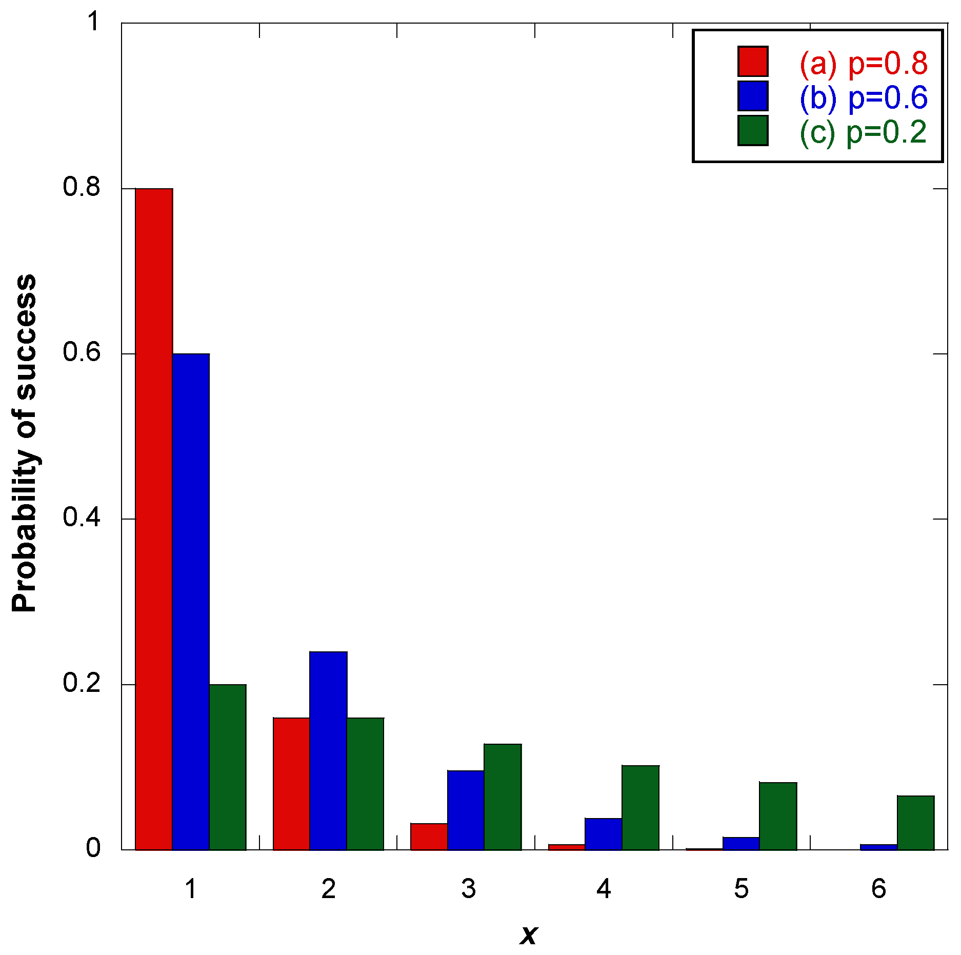
4. Geometric Distribution Approach

To tackle challenges arising from the biased node distribution, a novel algorithm designed to optimize the SF assignment for each node called the geometric distribution (GD) algorithm is proposed here. The geometric distribution is basically known as a discrete probability distribution used to model events with two outcomes in repeated trials until success is achieved. The Probability Mass Function (PMF) is a measure providing probabilities for possible values of a random variable. In an attempt to distribute the biased number of SF nodes, the probability of success rate (p-value) of the PMF is the key feature.

The PMF is presented in Equation (15). Notably, the PMF exhibits a distinct characteristic—the probability of success is the highest on the first trial (x = 1) and decreases in subsequent trials. The p-value is a crucial parameter ranging from 0 to 1, influencing the likelihood of success and the overall distribution of success rates. For example, if the p-value is less than 1, the probability of success will always be less than 1 regardless of the number of trials.

$$P\left(x\right)=(1-p{)}^{x-1}p, x=1, 2, 3, \dots$$

(15)

In an attempt to apply the GD to distribute the biased SF nodes, we defined two outcomes that are success and failure in distributing biased SF nodes to higher SF values. The p-value can be flexibly chosen to represent the desired probability of success. Since both node patterns shown in Table 2 are biased with SF7, the probability of success in the first trial, which is the highest, is certainly the assignment to SF7 nodes. Subsequent trials (x = 2–6) were assigned to SF8 through SF12, where the probability of success in distributing SF7 nodes to these higher SFs decreases monotonically at the fixed p-value. Figure 5 presents a visual representation of the probability of success derived from the GD PMF at p = 0.2, 0.6, and 0.8.

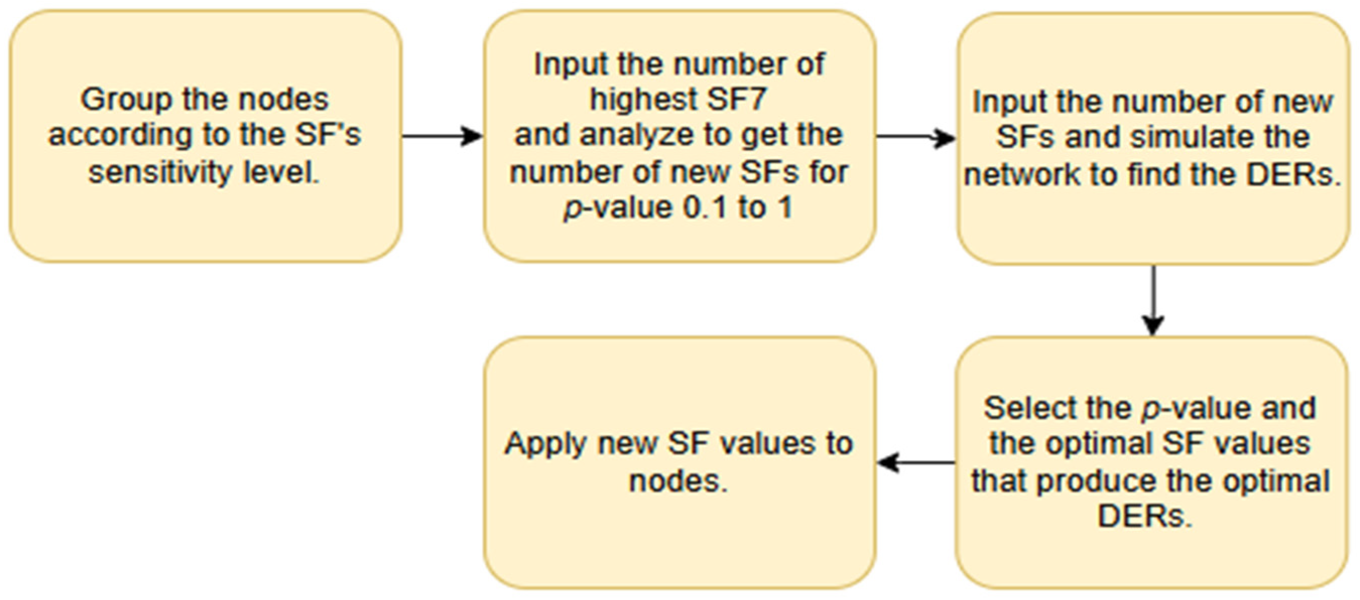
5. The Geometric Distribution Algorithm for SF Assignment

Reverting to the DER results run by the default ADR scheme, a significant challenge arose since more than 70% of all nodes from the uniform random and fixed patterns were assigned SF7 at 4 and 5 km. To significantly improve the DER, we needed to find the optimal SF distribution by redistributing the number of SF7 nodes using the PMF. Initially, we defined the probability of success p as the weight factor (w) for each SF. Then, we utilized the weight factor (w) to determine the number of SF nodes, as shown in Equations (16) and (17), respectively.

$$N_{SF \mathrm{m}\mathrm{a}\mathrm{x}}=w_1{N}_{SF \mathrm{m}\mathrm{a}\mathrm{x}}+w_2{N}_{SF \mathrm{m}\mathrm{a}\mathrm{x}}+\cdots +w_6{N}_{SF \mathrm{m}\mathrm{a}\mathrm{x}},$$

(16)

where N_{SF max} is the total number of majority SF nodes—in our case, SF7 nodes.

w_n is the weight factor of new SF7 (n = 1) to new SF12 (n = 6) and is defined as

$$w_n=p(1-p{)}^{n-1},$$

(17)

where n = 1–6.

Equation (16) is only valid when the summation of w₁ to w₆ is equal to 1—that is,

$$\sum _{n=1}^6{w}_n=\sum _{n=1}^{6}p(1-p{)}^{n-1}=1.$$

(18)

However, due to variation in the p-value, Equation (18) is not always summed to 1. To address this, a weight correction factor, calculated as the inverse of Equation (17), was multiplied to the right term of Equation (16). The corrected weight factor is

$$w_{n, corrected}={\displaystyle \frac{w_n}{{\sum }_{n=1}^6{w}_n}}.$$

(19)

For the sake of simplicity, we refer to the corrected weight factor by the original variable w for the rest of the paper. The numbers of new SF7–SF12 are obtained by multiplying w₁–w₆ in Equation (18) by N_{SF max}, respectively.

The GD algorithm was developed next and is shown in Algorithm 1. First, we input the highest number of nodes with a similar SF value, which in our case is SF7, to the proposed GD algorithm. Then, SF7 nodes were separated using the GD approach. The process entered a loop starting at p = 1, and the corresponding weight factors w[x] were multiplied by the SF7 count (N_{SF max}) to obtain the number of new SFs. The loop iterated as the p-value decreased by 0.1 decrement. The weight factors were recalculated at each p-value and, thus, the number of new SFs was obtained. The loop continued until the p-value reached 0.1, marking the end of the algorithm. Note that, although the 0.1 decrement was carefully selected to observe the overall SF variation characteristic, we added the calculation of weight factors at p-value = 0.005 to finely observe the SF variation when the p-value approaches the zero limit. The resulting set of weight factors at the p-value equaling 1 to 0.005 is presented in

Table 4. The resulting set of weight factor (w) with p-value = 1 to 0.005.

p-Value	w1	w2	w3	w4	w5	w6
1	1	0	0	0	0	0
0.9	0.90	0.09	0.01	0.00	0.00	0.00
0.8	0.80	0.16	0.03	0.01	0.00	0.00
0.7	0.70	0.21	0.06	0.02	0.01	0.00
0.6	0.60	0.24	0.10	0.04	0.02	0.01
0.5	0.51	0.25	0.13	0.06	0.03	0.02
0.4	0.42	0.25	0.15	0.09	0.05	0.03
0.3	0.34	0.24	0.17	0.12	0.08	0.06
0.2	0.27	0.22	0.17	0.14	0.11	0.09
0.1	0.21	0.19	0.17	0.16	0.14	0.13
0.005	0.17	0.17	0.17	0.17	0.17	0.16

.

Algorithm 1: Geometric distribution
1:	Input: Number of highest SF (NSF max)
2:	Define: Weight factor (w)
3:	Geometric distribution factor (p)
4:	Initialize: p = 1
5:	Do
6:	// Calculate the weight factor of each SF
7:	w[x] ← p × (1 − p) ^ (x − 1) let x = 1, 2, 3, 4, 5, 6
8:	// Calculate the number of each SF
9:	SF[y] ← NSF max × w[x] let x = 1, 2, 3, 4, 5, 6 and y = 7, 8, 9, 10, 11, 12
10:	// Return the new number of each SF
11:	Return SF [7], SF [8], SF [9], SF [10], SF [11], SF [12]
12:	p ← p − 0.1
13:	While p > 0.1 // p starts at 1 to 0.1, with 0.1 decrement

The complete implementation workflow is as shown in Figure 6. Initially, nodes were classified according to the sensitivity levels outlined in Figure 1. After applying the GD algorithm, the sets of weight-classified SF nodes were ingested into the simulation to determine Data Extraction Rate (DER) values for probabilities ranging from p = 1 to 0.1. Note that the DER is synonymous to the throughput in the sense that both terms refer to the amount of data successfully transferred from the source to its destination in a given timeframe. In our research, node and gateway represent such source and destination. The p-value that produced the optimal SF and DER values was selected, and finally, the optimized SF values were applied to the nodes.

6. Geometric Distribution Algorithm Performance Assessment

To assess the performance of the GD algorithm, we designed three experiments for network simulation with two node patterns: uniform random and fixed, as depicted in Figure 3 and Figure 4, respectively. Following this, we employed the LoRaSim simulator to generate the uniform random node pattern and to compute DER values for all experiments. Experiment 1 was the evaluation of the GD algorithm for both uniform random and fixed patterns. Experiment 2 was the comparison of the optimal SF assignment and corresponding DER values obtained from the GD algorithm and other previous works for both uniform random and fixed patterns. The parameters for experiments 1 and 2 were configured according to the specifications outlined in

Table 5. Simulation parameters.

Parameter	Value
Number of nodes	1500
Number of gateways	1
Node transmitted power	14 dBm
Simulation time	43,200 s (12 h)
Average sending message time	1800 s (30 min)
Bandwidth	125 kHz
Frequency (AS923)	923 MHz
Path-loss model	Suburban Hata–Okumura
Payload size	255 bytes
Coverage area	5 km

. The third experiment was the comparison of the GD algorithm-based network performance of the fixed pattern with the default ADR scheme [11] and previously reported algorithms—namely, EXPLoRa [14], QCVM [19], and SD [20]—by considering key parameters, namely, coverage area (2 to 5 km), payload size (10 to 255 bytes), and the total energy consumption during the simulation time from 1 to 12 h. Note that, since ADR is a default mechanism deployed by LoRaWAN, it serves well as a baseline for comparison with the GD algorithm. The EXPLoRA-SF or EXPLoRa, QCVM, and SD SF allocation schemes were selected due to their algorithmic simplicities being similar to the proposed GD algorithm. In particular, the QCVM and SD are also grounded in statistical techniques, making them suitable for comparison.

7. Results and Discussion

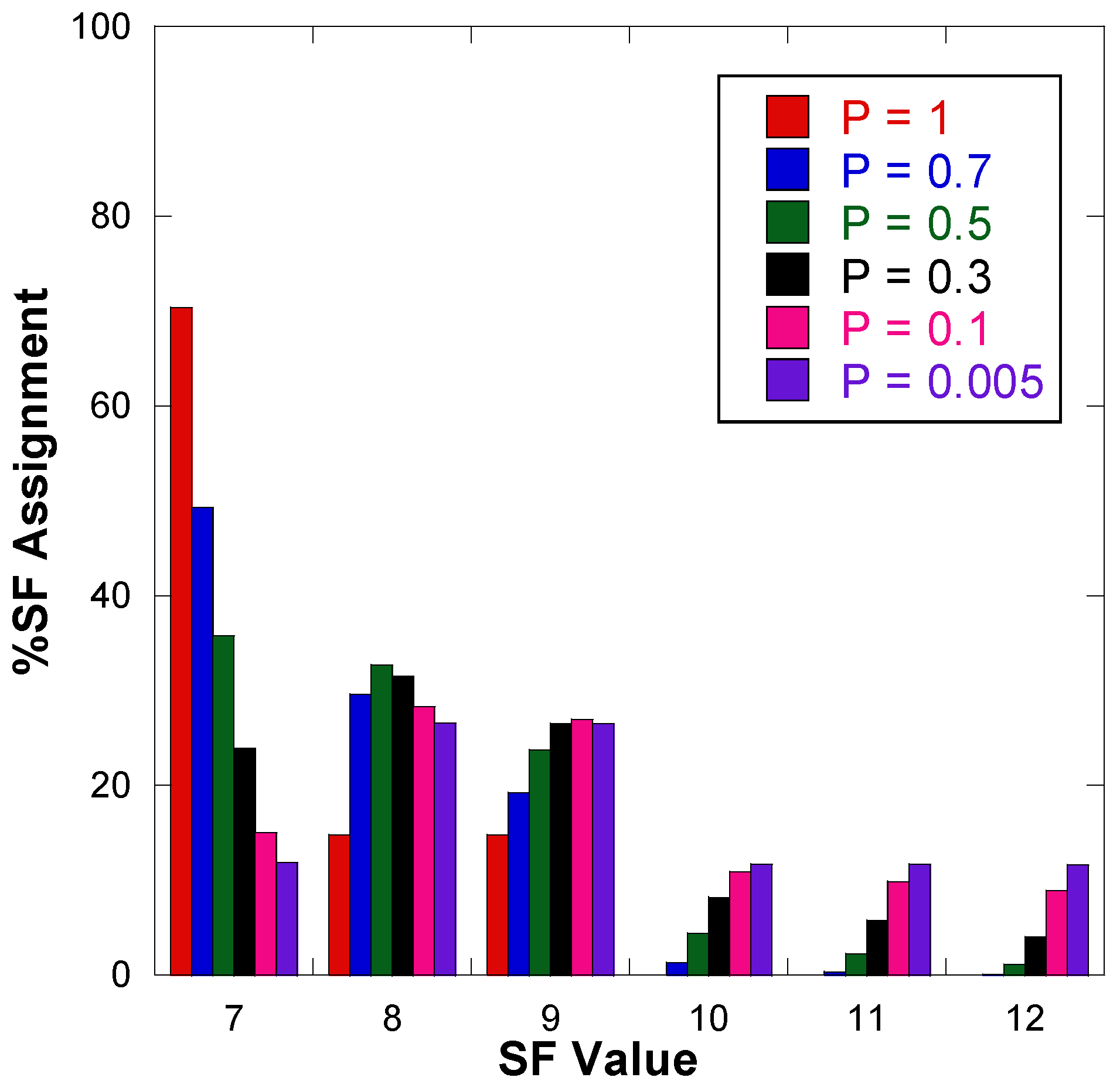
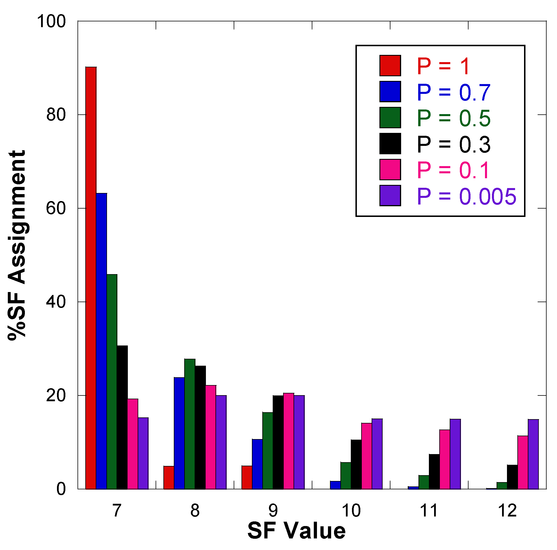
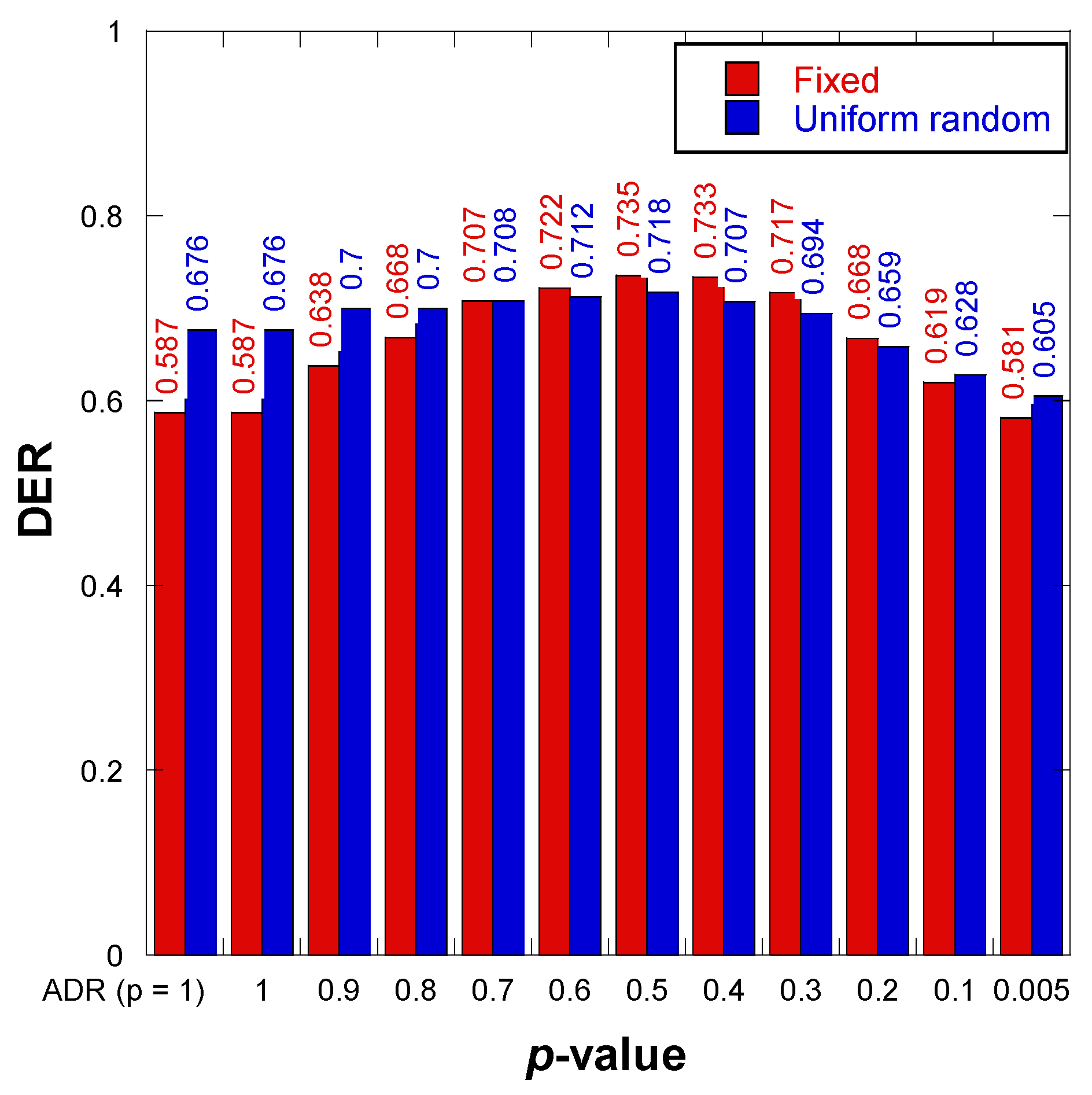
7.1. Experiment 1: Evaluation of the GD Algorithm for Uniform Random and Fixed Patterns

By using the GD algorithm, the new SF assignments for both uniform random and fixed patterns are presented in Figure 7 and Figure 8, respectively. For both patterns, the SF values are assigned across different probability values (p-value) ranging from 1 to 0.1. At p = 1, the SF distribution aligns with the default ADR scheme. As the p-value decreases, the number of SF7 nodes gradually separates into SF8-SF12 due to the weight factor (w).

By decreasing the p-value, the DER values of both patterns increase until reaching the optimal DER value at p = 0.5 and then decrease monotonically, as shown in Figure 9. The optimal DER value of the fixed pattern is approximately 73.5%, which is slightly better than that of the uniform random pattern (71.8%), and both DER values are clearly higher than the default ADR scheme. The numbers of new SFs for the uniform random and fixed patterns at p = 0.5 are shown as the bar graphs in Figure 7 and Figure 8, respectively. Note that the optimal p-values and corresponding DER values might be different for different node distributions.

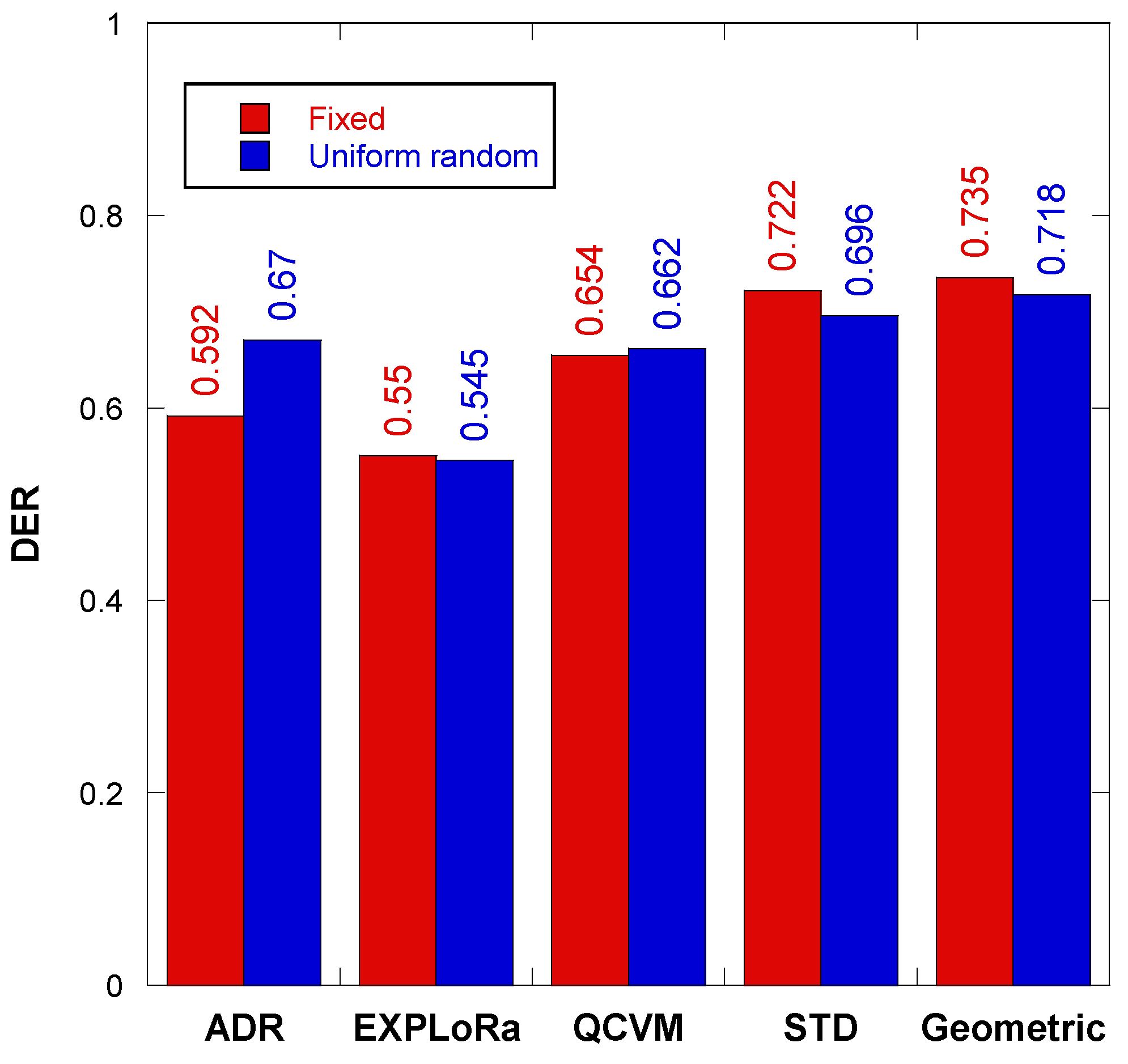
7.2. Experiment 2: Comparison of the GD Algorithm with Previous Reported Algorithms

In this experiment, the simulation was conducted to compare DER values between the GD algorithm at the optimal p = 0.5, the default ADR scheme [11], and previously reported algorithms, namely, EXPLoRa [14], QCVM [19], and SD [20].

Table 6. SF allocation from the GD algorithm at p = 0.5, default ADR scheme, and previous algorithms for the uniform random pattern.

Algorithm	%SF7	%SF8	%SF9	%SF10	%SF11	%SF12
Default ADR	70.00	16.53	13.47	0.00	0.00	0.00
EXPLoRa	16.67	16.67	16.67	16.67	16.67	16.67
QCVM	33.40	33.40	33.20	0.00	0.00	0.00
SD	25.60	37.47	14.27	14.47	6.33	1.87
GD (p = 0.5)	34.73	33.13	24.60	4.07	2.07	1.40

and

Table 7. SF allocation from the GD algorithm at p = 0.5, default ADR scheme, and previous algorithms for the fixed pattern.

Algorithm	%SF7	%SF8	%SF9	%SF10	%SF11	%SF12
Default ADR	89.67	5.40	4.93	0.00	0.00	0.00
EXPLoRa	16.67	16.67	16.67	16.67	16.67	16.67
QCVM	33.40	33.40	33.20	0.00	0.00	0.00
SD	35.20	32.73	17.33	12.67	1.33	0.73
GD (p = 0.5)	45.53	27.67	16.93	5.40	2.67	1.80

display the SF assignment for uniform random and fixed patterns, respectively. The result in Figure 10 clearly addresses a substantial impact of SF distribution on the DER value. Optimizing the SF distribution with the GD algorithm results in the overall highest DER, with a 4.8% and 14.3% improvement over the default ADR scheme for uniform random and fixed patterns, respectively.

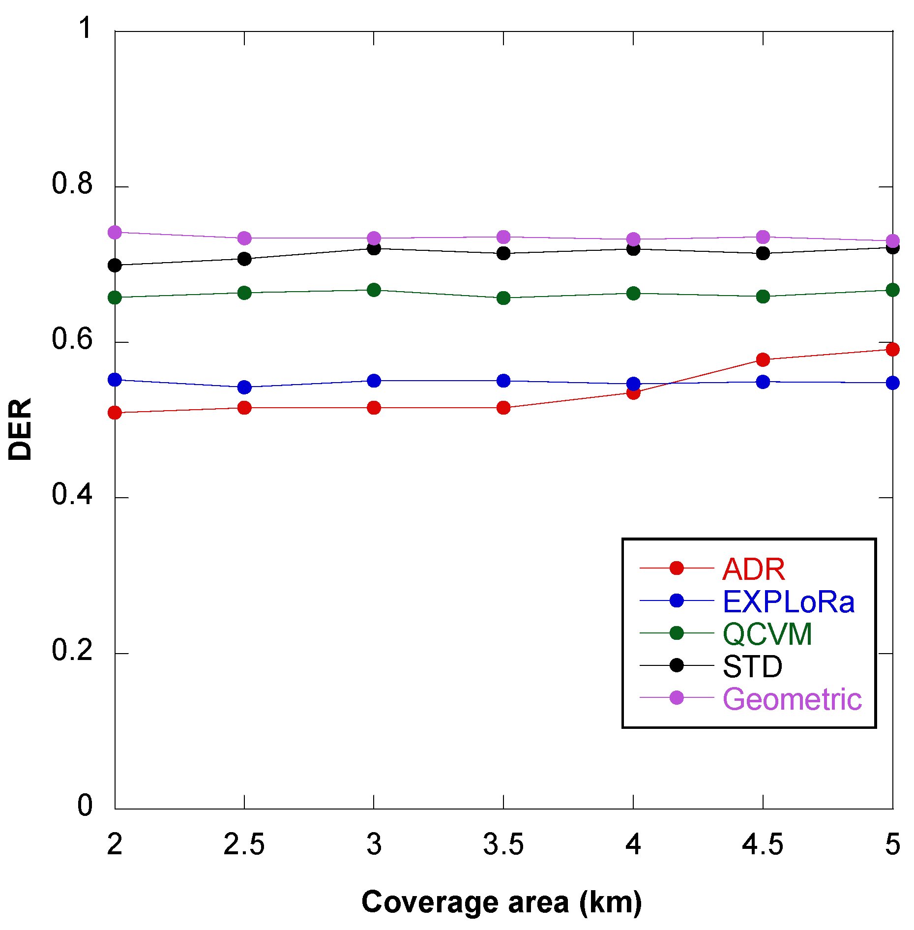
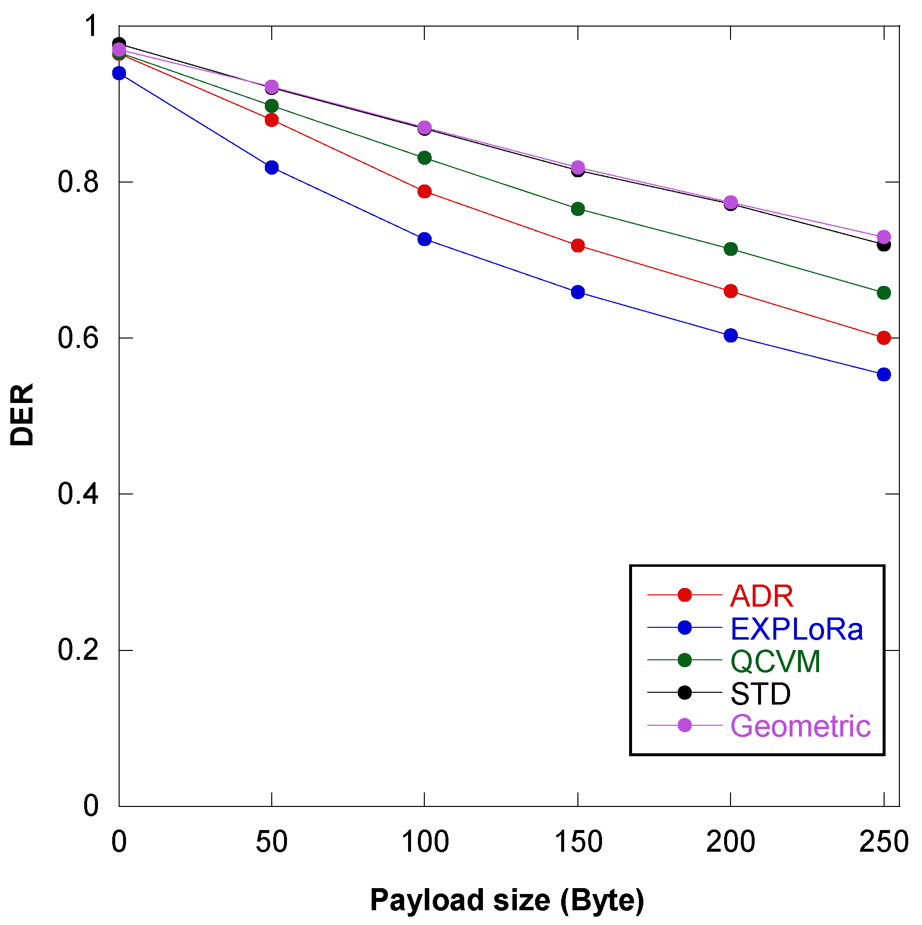
7.3. Experiment 3: Network Performance Evaluation of the GD Algorithm Based on Coverage Area, Payload Size, and Energy Consumption

We aimed at assessing the GD algorithm on the expansion of the coverage area as it is a crucial factor that influences SF assignment [19,20]. By expanding the coverage area from 2 to 5 km (to reflect the actual farm area), the proposed GD algorithm achieved a DER of 74%, higher than other algorithms, as shown in Figure 11. The DER of the default ADR scheme also improved at 4–5 km due to more node allocation to SF8 and SF9.

We also assessed the GD algorithm on the payload size, which plays an important role in defining the range of transmitted data. From Figure 12, a decline in DER as the payload size increases is observed for all algorithms. Remarkably, the proposed algorithm demonstrates notable improvement, surpassing the default ADR scheme by more than 13% at a payload size of 255 bytes. This finding indicates the potential of the GD algorithm to successfully carry the larger load over the air.

Node energy consumption is primarily influenced by Time-on-Air (ToA) and node power. As shown in Equations (4) and (5), ToA is a function of spreading factor (SF), implying that different SF allocation algorithms will result in varying ToA and, thus, node energy consumption. Figure 13 shows the total ToA when increasing the simulation time from 1 h to 12 h. While gateway and server energy consumption in existing LoRaWAN networks remains largely unaffected by SF allocation algorithms, node energy consumption is a significant factor differentiating the overall network energy usage.

Figure 14 displays the total energy consumption when increasing the simulation time from 1 h to 12 h. Since ToA increases with the SF value, the SF assignments can then be used to justify the results. For EXPloRa, where there is a greater number of large SF nodes, the energy consumption is clearly higher than other algorithms. On the other hand, the default ADR scheme offers the lowest energy consumption as almost 90% of the nodes are SF7. The proposed GD algorithm offers relatively the same energy consumption as the SD but slightly higher than that of the QCVM due to neither SF10, SF11, nor SF12 being assigned for QCVM.

8. Conclusions

This research endeavored to enhance the performance of the LoRaWAN by addressing collision probability issues, specifically aiming to reduce instances of the same SF. Various algorithms employed in the past often incorporated RSSI optimization on random and normally distributed node patterns. Our contribution to this domain introduced a novel algorithm based on the geometric distribution (GD), where we applied this algorithm to real-world scenarios that possessed certain node patterns with biased SFs. One outstanding attribute of the GD algorithm is its adaptability in selecting the weight factor (w) through the p-value, allowing for precise customization of SF distribution. Results from our study indicated that the proposed algorithm achieved significant improvements in both optimal SF assignment and DER values compared to previous algorithms. Specifically, the fixed pattern exhibited an impressive enhancement of 14.3%, while the uniform random pattern exhibited a 4.8% enhancement over the default ADR scheme.

Expanding the coverage area and increasing the package size further underscored the efficacy of the proposed algorithm, consistently yielding the highest DER values. However, it was important to note that achieving these improvements required allowing higher energy consumption and time-on-air since larger SF values were also assigned. To effectively manage energy consumption, it is advisable to limit the proportion of larger SFs. However, this may inevitably impact the DER. Consequently, a careful balance between DER and energy consumption must be considered, necessitating appropriate adjustments to the algorithm.

Additionally, as highlighted in a previous study [19], the GD algorithm’s performance may be less optimal in environments with uniformly distributed or non-dominant SFs. To address this limitation, a preliminary assessment of the node distribution pattern could be conducted using an additional function within the algorithm.

Looking ahead, the GD algorithm emerges as a valuable tool for resource allocation, especially in scenarios where there are mostly the same SF nodes in one area. This algorithm holds promise for optimizing resource distribution and finding the most efficient pathways. To enhance the GD algorithm’s performance, integrating machine learning techniques such as long short-term memory (LSTM) and deep learning [27] could be beneficial. LSTM can be used to predict energy consumption patterns, enabling more efficient packet transmission timing and reducing overall energy consumption. Deep learning can be applied to optimize coverage capacity by leveraging LoRaWAN traffic models. Decentralized approaches employing multi-class support vector machines (SVMs) and artificial neural networks (ANNs) [28] can be applied to effectively allocate nodes into clusters for optimal SF allocation. Additionally, a deep generative model like the variational autoencoder (VAE) model [29] can be applied to identify the optimal SF settings for various scenarios by simplifying the complex relationships between different parameters that affect SF allocation.

These advancements could potentially expand the applicability of this algorithm beyond LoRaWAN to other wireless communication technologies, including Sigfox, Wi-Fi, and 5G. The adaptability and effectiveness of the geometric distribution algorithm position it as a potential solution for future advancements in long-range wireless communication optimization.

References

1. Augustin, A.; Yi, J.; Clausen, T.; Townsley, W.M. A Study of LoRa: Long Range & Low Power Networks for the Internet of Things. Sensors 2016, 16, 1466. [Google Scholar] [CrossRef] [PubMed]
2. Haxhibeqiri, J.; De Poorter, E.; Moerman, I.; Hoebeke, J. A Survey of LoRaWAN for IoT: From Technology to Application. Sensors 2018, 18, 3995. [Google Scholar] [CrossRef] [PubMed]
3. Mwakwata, C.B.; Malik, H.; Mahtab Alam, M.; Le Moullec, Y.; Parand, S.; Mumtaz, S. Narrowband Internet of Things (NB-IoT): From Physical (PHY) and Media Access Control (MAC) Layers Perspectives. Sensors 2019, 19, 2613. [Google Scholar] [CrossRef] [PubMed]
4. Sigfox. Available online: https://www.sigfox.com (accessed on 14 November 2019).
5. Mohamad, M. Performance Analysis of Air Monitoring System Using 433 MHz LoRa Module. Prz. Elektrotech. 2024, 1, 225–229. [Google Scholar] [CrossRef]
6. Sujono, H. Drip Irrigation Control System Based on Mamdani Fuzzy Logic and Internet of Things (IoT). Prz. Elektrotech. 2024, 1, 65–69. [Google Scholar] [CrossRef]
7. Boonsong, W. Proposed Precision Analysis of Water Quality Monitoring Embedded IoT Network. Prz. Elektrotech. 2023, 1, 177–180. [Google Scholar] [CrossRef]
8. Sambor, S. Przykład Zastosowania Sieci LoRaWAN do Monitorowania Parametrów Środowiskowych w Budynku Wielkopowierzchniowym. Prz. Elektrotech. 2022, 1, 29–34. [Google Scholar] [CrossRef]
9. Zankiewicz, A. Eksperymentalna Analiza Efektywności Transmisji Danych w Sieci LoRaWAN w Eksploatacji na Terenie Miejskim. Prz. Elektrotech. 2023, 1, 43–50. [Google Scholar] [CrossRef]
10. El Chall, R.; Lahoud, S.; El Helou, M. LoRaWAN Network: Radio Propagation Models and Performance Evaluation in Various Environments in Lebanon. IEEE Internet Things J. 2019, 6, 2366–2378. [Google Scholar] [CrossRef]
11. Semtech Corporation. Understanding the LoRa Adaptive Data Rate. Available online: https://learn.semtech.com/mod/page/view.php?id=136 (accessed on 20 December 2019).
12. Mahmood, A.; Ge Sisinni, E.; Guntupalli, L.; Rondon, R.; Hassan, S.A.; Gidlund, M. Scalability Analysis of a LoRa Network under Imperfect Orthogonality. IEEE Trans. Ind. Inform. 2019, 15, 1425–1436. [Google Scholar] [CrossRef]
13. Saluja, D.; Singh, R.; Baghel, L.K.; Kumar, S. Scalability Analysis of LoRa Network for SNR-Based SF Allocation Scheme. IEEE Trans. Ind. Inform. 2021, 17, 6709–6719. [Google Scholar] [CrossRef]
14. Al-Gumaei, Y.A.; Aslam, N.; Chen, X.; Raza, M.; Ansari, R.I. Optimizing Power Allocation in LoRaWAN IoT Applications. IEEE Internet Things J. 2022, 9, 3429–3442. [Google Scholar] [CrossRef]
15. Cuomo, F.; Campo, M.; Caponi, A.; Bianchi, G.; Rossini, G.; Pisani, P. EXPLoRa: Extending the Performance of LoRa by Suitable Spreading Factor Allocations. In Proceedings of the 2017 IEEE 13th International Conference on Wireless and Mobile Computing, Networking and Communications (WiMob), Rome, Italy, 9–11 October 2017; pp. 1–8. [Google Scholar] [CrossRef]
16. Garlisi, D.; Tinnirello, I.; Bianchi, G.; Cuomo, F. Capture Aware Sequential Waterfilling for LoRaWAN Adaptive Data Rate. IEEE Trans. Wirel. Commun. 2021, 20, 2019–2033. [Google Scholar] [CrossRef]
17. Hong, S.; Yao, F.; Zhang, F.; Ding, Y.; Yang, S.-H. Reinforcement Learning Approach for SF Allocation in LoRa Network. IEEE Internet Things J. 2023, 10, 18259–18272. [Google Scholar] [CrossRef]
18. Usama Minhaj, S.; Mahmood, A.; Fakhrul Abedin, S.; Ali Hassan, S.; Talha Bhatti, M.; Ali, S.; Gidlund, M. Intelligent Resource Allocation in LoRaWAN Using Machine Learning Techniques. IEEE Access 2023, 11, 10092–10106. [Google Scholar] [CrossRef]
19. Tempiem, P.; Silapunt, R. Quantile Classification of Variance from the Mean for Spreading Factor Allocation in LoRaWAN. In Proceedings of the 2020 5th International Conference on Information Technology (InCIT), Chonburi, Thailand, 21–22 October 2020; pp. 179–184. [Google Scholar] [CrossRef]
20. Tempiem, P.; Silapunt, R. Spreading Factor Allocation Using the Standard Deviation Classification Method. In Proceedings of the 2020 International Symposium on Antennas and Propagation (ISAP), Osaka, Japan, 25–28 January 2021; pp. 145–146. [Google Scholar] [CrossRef]
21. Poluektov, D.; Polovov, M.; Kharin, P.; Štůsek, M.; Zeman, K.; Masek, P.; Kochetkova, I.; Hosek, J.; Samouylov, K. On the Performance of LoRaWAN in Smart City: End-Device Design and Communication Coverage. In Distributed Computer and Communication Networks; Springer: Cham, Switzerland, 2019. [Google Scholar] [CrossRef]
22. Harinda, E.; Hosseinzadeh, S.; Larijani, H.; Gibson, R.M. Comparative Performance Analysis of Empirical Propagation Models for LoRaWAN 868MHz in an Urban Scenario. In Proceedings of the 2019 IEEE 5th World Forum on Internet of Things (WF-IoT), Limerick, Ireland, 15–18 April 2019; pp. 154–159. [Google Scholar] [CrossRef]
23. Kamonkusonman, K.; Phunthawornwong, M.; Tempiem, P.; Silapunt, R. Utilization-Weighted Algorithm for LoRaWAN Capacity Improvement for Local Smart Dairy Farms in Ratchaburi Province of Thailand. IEEE Access 2021, 9, 141738–141746. [Google Scholar] [CrossRef]
24. Britannica. Geometric Distribution Probability. Available online: https://www.britannica.com/topic/geometric-distribution (accessed on 14 February 2024).
25. Maurya, P.; Singh, A.; Kherani, A.A. A Review: Spreading factor allocation schemes for LoRaWAN. Telecommun. Syst. 2022, 80, 449–468. [Google Scholar] [CrossRef]
26. Molisch, A.F. Wireless Communications Handbook; John Wiley & Sons: Hoboken, NJ, USA, 2011. [Google Scholar]
27. Morariu, C.; Morariu, O.; Răileanu, S.; Borangiu, T. Machine learning for predictive scheduling and resource allocation in large scale manufacturing systems. Comput. Ind. 2020, 120, 103244. [Google Scholar] [CrossRef]
28. Luo, F.L. Machine Learning for Optimal Resource Allocation. In Machine Learning for Future Wireless Communications; Wiley-IEEE Press: Hoboken, NJ, USA, 2020; pp. 85–103. [Google Scholar] [CrossRef]
29. Mak, H.W.L.; Han, R.; Yin, H.H.F. Application of Variational AutoEncoder (VAE) Model and Image Processing Approaches in Game Design. Sensors 2023, 23, 3457. [Google Scholar] [CrossRef] [PubMed]
Figure 1. Relationship of SF, data rate, ToA, energy consumption, and sensitivity level.
Telecom 05 00047 g001
Figure 3. Uniform random node pattern.
Telecom 05 00047 g003
Figure 4. Fixed node pattern.
Telecom 05 00047 g004
Figure 5. The probability of success from the GD PMF.
Telecom 05 00047 g005
Figure 6. GD algorithm-based SF assignment workflow.
Telecom 05 00047 g006
Figure 7. SF assignment for the uniform random pattern using the GD algorithm.
Telecom 05 00047 g007
Figure 8. SF assignment for the fixed pattern using the GD algorithm.
Telecom 05 00047 g008
Figure 9. DER values after applying the GD algorithm to the fixed and uniform random patterns.
Telecom 05 00047 g009
Figure 10. DER comparison between different algorithms for fixed and uniform random patterns.
Telecom 05 00047 g010
Figure 11. The DER values vs. the coverage area within different algorithms.
Telecom 05 00047 g011
Figure 12. The DER values vs. the payload size (bytes) within different algorithms.
Telecom 05 00047 g012
Figure 13. Time-on-Air from 1 h to 12 h of simulation time within different algorithms.
Telecom 05 00047 g013
Figure 14. Energy consumptions from 1 h to 12 h of simulation time within different algorithms.
Telecom 05 00047 g014