Abstract
Fingerprinting-based positioning exploiting in two dimensions the spatial side information on fingerprints from adjacent positions relative to a target position is studied. The positioning is performed at the positioning device, utilizing as fingerprints the received signal strengths of downlink radio signals, collected using a two-dimensional sensor array. The motivation is to minimize the positioning error by transferring the complexity and cost from the infrastructure to the positioning device. The goal is to learn whether spatial side information on the fingerprints can minimize the positioning error. We provide a differentiation between fingerprinting in uplink and downlink, a classification of the positioning data aggregation domains, concepts, and a related literature review. We present three pattern-matching methods for estimating the position using spatial side information, two based on regression, implemented using feedforward neural networks, and one based on classification of the fractions of the positioning area, implemented using a convolutional neural network. Fingerprinting with and without spatial side information is benchmarked using the proposed pattern-matching methods in a system simulator based on Monte Carlo methods, generating synthetic fingerprints with an indoor radio channel model and calculating the positioning error. It is observed that for the given assumptions and the system considered, fingerprinting-based positioning with spatial side information substantially reduces the positioning error.
Keywords:
fingerprinting-based positioning; localization; spatial side information; machine learning; Monte Carlo system simulations; downlink received signal strength; two-dimensional sensor array; integrated sensing and communications; large reconfigurable intelligent surfaces; synthetic image generation 1. Introduction
Positioning systems form the core or a complementary part of other systems. When combined with radio networks, the integration of communications and sensing opens new possibilities to enable functions and services in the control and user planes. The convergence of communications and sensing [1] defines a new paradigm referred to as Integrated Sensing and Communications (ISAC) [2,3,4].
Global Navigation Satellite Systems (GNSSs) are used mainly for outdoor positioning, where there is a Line of Sight (LOS) between a positioning device and the satellites that form part of the positioning system’s infrastructure. For cases where there is no LOS, for example, at indoor locations, an alternative positioning system is required.
General compendiums on the positioning systems, methods, and technologies for indoor and outdoor use are described in [5,6,7,8,9,10,11,12,13,14,15]. In the context of this work, we will primarily cover indoor positioning systems, although the approach to be described can be implemented for outdoor use-cases as well. Among the different positioning methods and technologies for indoor positioning, we will discuss fingerprinting-based positioning. It is outside of our scope to argue for the benefits and drawbacks of each positioning method and technology, as these have been widely discussed in the literature. In our view, each positioning method and technology has its merits, problems, and an associated cost–performance or cost–benefit. Here, we focus on enhancing fingerprinting-based positioning.
Fingerprinting-based positioning uses the magnitudes of signals that vary as function of position, called fingerprints, so that these can be mapped to an approximate position estimate. Fingerprinting-based positioning can be used (1) as a positioning method alone; (2) to complement other positioning methods in a so-called hybrid positioning system; (3) to act as a secondary positioning system to back up a primary positioning system; (4) to make an assessment or evaluate the trustworthiness of the position reported by a primary positioning system; or (5) as part of a collaborative positioning system [16].
A common metric of performance used in positioning systems is the positioning error referred to as the distance error or error distance. In the context of our work, the positioning error is defined as the Euclidean distance measured from the position reported by a positioning device to a known ground truth reference position. An ideal positioning system would be one in which the positioning error is minimized to zero. However, in practice, the minimization of the positioning error has an associated complexity and cost.
The costs in positioning systems primarily comprise the capital and maintenance costs of the core infrastructure and positioning devices. In addition, there are costs associated with the time required to install and configure a positioning system, the data post-processing time, and the computing time. Some of the costs involved in a positioning system are discussed in [17]. All of these costs are summarized in some contexts as the total cost of ownership.
Among different positioning methods, fingerprinting-based positioning is generally regarded as an economical option. Its low cost can be attributed to different reasons. One reason is the possibility of relying on signals, or any other distinctive characteristic of the environment, which can be repurposed as fingerprints for positioning when these are available in the area where the positioning is needed (e.g., magnetic fields, sounds, radio signals, etc.). Another reason is the fact that this method does not require knowledge of the position of the sources that generate the fingerprints. This fact minimizes the costs of infrastructure and the coordination to set up the positioning system.
The sources that generate the fingerprints can be managed or unmanaged. In a managed approach to the fingerprint sources, there may be no knowledge of the actual position of the fingerprint sources, but there is knowledge of their status, at least for long periods of time. This status comprises the knowledge that a fingerprint source remains in the same place and the knowledge that it remains available. A typical example is the case of fingerprints from radio signals, which originate from transmitters operating in licensed radio frequency bands. In the case of cellular radio communication networks, the allocation of the frequency bands and the location of base stations for macro-cells and pico-cells do not change too often. An operator of the network, or a third party with an agreement with the network operator, can rely on using fingerprint sources with knowledge of their status. Management of the fingerprint sources contributes to their reliability, minimization of the positioning errors, and the lower costs of maintaining databases of the fingerprints. In contrast, in an unmanaged approach to the fingerprint sources, any suitable signal that is available in the environment is repurposed as a fingerprint. In this case, it is not granted that the source of the signal will remain in the same place and/or that the signal will remain available or retain the same characteristics. This is the case most commonly found in the literature related to fingerprinting-based positioning. This approach strives for economy on the positioning infrastructure side, traded off against its lower reliability and possibly larger positioning errors. Yet in the unmanaged case, the infrastructure costs may be negligible, such as in the case of using radio signals from unmanaged wireless local access networks as fingerprints.
Two main parts can be distinguished in a positioning system, namely the core positioning system infrastructure and the actual positioning device. In the context of fingerprintingbased positioning, the core positioning system infrastructure is composed mainly of positioning nodes or anchors. In the case of fingerprinting-based positioning using radio signals as fingerprints, the nodes are the sources (transmitters) that generate the fingerprints in the downlink case or the devices (receivers) that receive the fingerprints in the uplink case.
In order to minimize the positioning error, it is possible to increase the complexity and cost of the core positioning system infrastructure, the positioning device, or both.
In fingerprinting-based positioning, a typical way to minimize the positioning error is to increase the cost and complexity in the positioning system core infrastructure by increasing the number, and thus the density, of positioning nodes; see Figure 1a. In some cases, densification of the positioning nodes has an associated cost of attaching positioning nodes to buildings, structures, etc. Some examples are contexts like tall structures or mines [17,18], where not only is certain special equipment needed for maintenance (e.g., cranes) but also only qualified personnel are allowed to reach these places. From another perspective, in some industries, the costs of cabling (data/power) may increase noticeably, for example, when requiring sealed pipes for electrical wiring in hazardous areas. Even when wireless and battery-operated positioning nodes are an option in hazardous areas and places that are difficult to reach, these have an associated maintenance cost that cannot be neglected as part of the total cost of ownership in the corresponding business models.
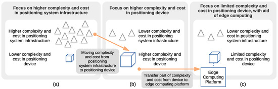
Figure 1.
Focus on higher complexity and cost in (a) positioning system infrastructure, (b) positioning device, and (c) positioning device with support of edge computing.
Returning to the complexity and cost alternatives, another alternative for minimizing the positioning error is to increase the complexity and cost in the positioning device while decreasing the cost and complexity in the positioning system core infrastructure; see Figure 1b. This solution may be justified in situations where the increment in the costs associated with the positioning device is smaller when compared to the costs associated with the positioning infrastructure. For this alternative, there are use-cases where it is justified to move the complexity and cost from the core infrastructure to the positioning device. This transition of the complexity and cost is depicted by the arrow pointing from the case in Figure 1a to the case in Figure 1b.
With the arrival of the edge computing paradigm [19,20], an alternative solution to the two presented above consists of transferring part of the complexity of the positioning device to an edge computing platform; see Figure 1c. It is outside of our scope to discuss whether an edge computing platform is considered to be part of the positioning infrastructure or not. An example of its use would be to decrease the complexity and cost of the core infrastructure by avoiding densification of the positioning nodes, increasing the hardware complexity at the positioning device, and complementing it with computing resources from edge computing platforms. This third option is presented to put our work into context and to pave the way for future related work. For example, the case depicted in Figure 1c can be thought of as an extension of the case depicted in Figure 1b. In the context of this work, we focus solely on the case depicted in Figure 1b.
In this paper, we propose minimizing the positioning error in fingerprinting-based positioning by increasing the complexity on the positioning device side, as depicted in Figure 1b, exploiting fingerprints in two spatial dimensions. We work with received signal strength (RSS) fingerprints in a radio network scenario operating in downlink. We propose using a two-dimensional (2D) array arrangement of sensors (e.g., antennas and receivers), referred to as a 2D sensor array, that allows us to measure physically adjacent fingerprints. This arrangement provides 2D spatial side information on the fingerprints at the positioning device. Our primary goal is to learn whether using spatial side information on RSS fingerprints, by means of an ideal 2D sensor array, could lead to a justifiable gain in terms of minimizing the positioning error. Spatial side information is introduced in Section 2.5.
An example of the proposed 2D sensor array is depicted in Figure 2. The fingerprints measured by the 2D sensor array will be associated with small discretized areas of the same size as the 2D sensor array.
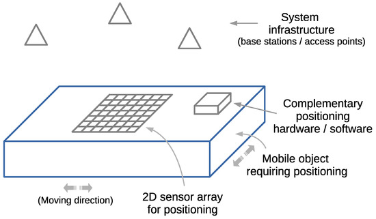
Figure 2.
Representative view of a mobile object requiring positioning and implementing a 2D sensor array for fingerprinting-based positioning.
The idea is to scan during a training phase the whole main area where the positioning takes place, as takes place in traditional fingerprinting-based positioning, ideally covering the entire positioning area in pieces equivalent to the size of the 2D sensor array. The positioning area is defined, in general terms, as the area where the positioning is intended. Specifically in the context of the scenario and simulator used in this work, the positioning area is defined and explained in Section 5.1.
We carry out a feasibility study through simulations using a system simulator to learn whether the proposed approach could lead to a justifiable gain. This study is performed using simulations based on Monte Carlo methods, testing the performance of the proposed approach at random positions in terms of measuring the positioning error. The system simulator creates synthetic fingerprints in the form of RSS signals, with a radio channel model published by a standardization body for a frequency of GHz (other frequencies can be considered, see Section 5.9). We investigate four pattern-matching methods for processing the fingerprints based on machine learning algorithms for supervised learning, implemented with artificial neural networks (NNs). The first method is the traditional fingerprinting method, which associates a single vector of fingerprints with the position to be estimated, and thus has no spatial side information. The second method is based on regression; it exploits the spatial side information by aggregating the position estimates of the first method for all of the points associated with the 2D sensor array. The third and fourth methods exploit the spatial side information from the fingerprint data from the 2D sensor array in the method itself, that is, before mapping these to a position estimate. The third method is based on regression, implementing a feedforward neural network (FFNN). The fourth method is based on classification of the discretized areas associated with the 2D sensor array, implementing a convolutional neural network (CNN). The fourth pattern-matching method was implemented conjecturing that a pattern-matching method based on the classification of the discretized areas could be applied to estimating the position. We verify through the simulations whether this conjecture holds and whether it allows us to enhance the position estimates when compared with those of the other methods. The performance of the last three methods, using spatial side information, is benchmarked against that of the first method, which is regarded as the common state-of-the-art for estimating a position in fingerprinting-based positioning.
Through the use of the proposed pattern-matching methods, we aim as our primary goal to learn whether the use of spatial side information brings some gain. Our secondary goal is to learn how the different pattern-matching methods that process the side information perform against each other. As an additional goal, we are interested in the exploitation of the spatial side information before the fingerprints are mapped to an estimated position using a pattern-matching method, in a so-called fingerprint domain. In this context, two of the pattern-matching methods proposed are designed to exploit the fingerprints from the target and adjacent spatial positions in the fingerprint domain.
To the best of our knowledge, there are no previous works addressing the use of spatial side information as is proposed in this article.
Our main contributions are the following:
- The proposal to transfer the complexity and cost from the infrastructure side to a positioning device.
- Differentiation between uplink and downlink cases for fingerprinting-based positioning, relating Multiple-Input Multiple-Output (MIMO), massive MIMO, and intelligent surfaces.
- Differentiation between positioning data aggregation in the fingerprint and position domains.
- The proposal to collect the fingerprints at adjacent positions relative to a target position by means of a 2D sensor array located at the positioning device.
- The proposal to use 2D spatial side information from the fingerprints collected by the 2D sensor array to minimize the positioning error.
- The aggregation of the fingerprinting data from adjacent spatial positions prior to the mapping from the fingerprints to a position estimate.
- The conjecture that a pattern-matching method based on the classification of the discretized areas can be applied to estimating the position.
- Three pattern-matching methods for estimating the position by processing the fingerprints with spatial side information. Two methods are based on regression, implemented using FFNNs, and one method is based on the classification of fractions of the positioning area, implemented using a CNN. In turn, one method operates with data in the so-called position domain, and the other two methods operate with data in the so-called fingerprint domain.
- A feasibility study, for a given scenario and assumptions, using system simulations based on Monte Carlo methods.
- Benchmarking of cases without and with spatial side information.
- Benchmarking of the CNN-based method to determine whether it allows us to enhance the position estimates when compared with those from other methods.
The structure of this article is as follows. In Section 2, we introduce fingerprinting-based positioning, discuss mobile-device-based positioning, describe the positioning data aggregation domains, introduce spatial side information, and summarize the key assumptions and scope. In Section 3, we review the literature, identifying previous work proposing the use of spatial side information on the device side with downlink transmission. In Section 4, we explain the concept of fingerprinting with spatial side information and introduce a two-dimensional sensor array, the discretization of the positioning area into area fractions, the positioning process, and the selected pattern-matching methods. The feasibility study using system simulations is presented in Section 5, comprising the generation of the datasets of fingerprints, the implementation of the radio channel model, the simulation process, and simulation execution. The results of the simulations are summarized in Section 6. In Section 7, our conclusions are drawn, the results are discussed, and directions for future work are presented.
Example of a Hybrid Positioning System
LiDAR produces position estimates in local reference coordinates with a small positioning error compared to that with other methods. In practice, LiDAR is complemented by simultaneous localization and mapping algorithms to keep track of the location and assisted with a global reference to map local coordinates into global coordinates. One approach consists of constructing maps, in a so-called place recognition step, followed by a second step performing a pose estimation [21,22]. However, in some environments with multiple repetitive structural patterns, such as buildings without distinctive indoor characteristics, corridors, or tunnels, it is challenging to keep track of the position. In addition, if a positioning system is suddenly turned on, or reset, in such environments, it is difficult to determine a reference global position without further assistance. In these cases, a possible solution is to complement the place recognition with input of the global position estimates produced using fingerprinting-based positioning, thus assisting LiDAR in mapping its local position coordinates into global coordinates. The sensor array described in this article could be used to assist in the mapping of local to global coordinates, as well as in producing an estimate of the heading information in a single measurement.
2. Basic Concepts and Work Scope
In the next subsections, we review the concepts necessary for understanding and putting our work into context, define the terminology, and explain the intended scope.
2.1. Acronyms Used in the Article
Table 1 lists the acronyms of general use used in this article. Acronyms specific to the datasets used in this study are described in Section 5.2.

Table 1.
Acronyms of general use in the article.
2.2. Fingerprinting-Based Positioning
Fingerprinting-based positioning is based on the ideal assumption that fingerprints, with these being a physical signal or any distinctive characteristic of the environment, alone or in a set, can be associated with a unique position in space. Figure 3 shows an example of fingerprints from three sources for positioning in 2D. In this figure, the fingerprints from each source are represented as a three-dimensional (3D) continuous surface, in which a fingerprint measure is a function of 2D position coordinates. A position is represented by an ideally unique combination of fingerprints. In practice, the presence of noise, interference, and other disturbances results in position estimates that contain a certain degree of positioning error.
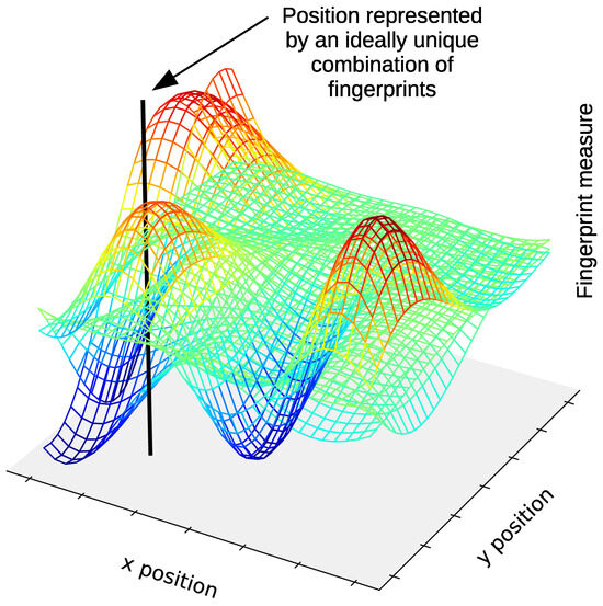
Figure 3.
Example of fingerprints from three sources for positioning in 2D. The fingerprints from each source are represented as a 3D continuous surface, where the fingerprint measure is a function of the position coordinates. A position is represented by an ideally unique combination of fingerprints.
Different kinds of fingerprint sources are reported in the literature, for example, visible light [23,24,25], Fine Timing Measurement (FTM) ranging values [26], ultra-wideband signals [27], sound [28,29], magnetic fields [30,31], Channel State Information (CSI) [32] (and the references in Section 3.1 and Section 3.2), and RSS (references in Section 3.1 and Section 3.2). In addition, some authors treat visual images as fingerprints (see [33] and the references therein).
Different types of fingerprints are, in some cases, combined together or are combined with other positioning methods through data fusion or other techniques to form hybrid positioning systems. For example, in [34], magnetic field fingerprints are fused with visual images, while in [35], the CSI amplitude is combined with the RSS.
Fingerprinting-based positioning consists of two stages or phases. The first phase is commonly known in the literature as the offline or training phase. It consists of gathering fingerprints and constructing a suitable mapping from a sampled set of fingerprints to a ground truth reference position by means of a pattern-matching method. The ground truth position is usually obtained by other means in this phase, for example, with the aid of a secondary positioning system that it is known to produce a smaller positioning error. In Figure 4 (left), the training phase is represented in the case of a pattern-matching method based on supervised learning with an NN.
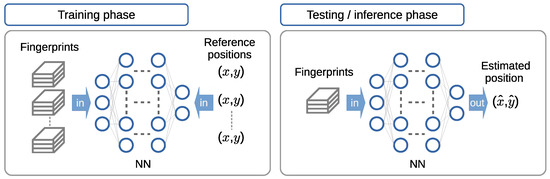
Figure 4.
Distinction between the training and testing phases (left and right subfigures, respectively) in fingerprinting-based positioning, with a pattern-matching method based on supervised learning using a neural network (NN).
A second phase, known in the literature on fingerprinting-based positioning as the online or testing phase, consists of mapping an input set of fingerprints to an output estimate of position coordinates, as depicted in Figure 4 (right) The mapping is performed using the pattern-matching method constructed or trained in the training phase. In the context of deep learning methods, this phase is referred to as the inference phase. In the inference phase, a trained NN model is used to make predictions based on input data. Hereafter, we refer to this phase as the testing phase, which is the terminology mainly used in the field of fingerprinting-based positioning and its literature. As all of the pattern-matching methods considered in this article are based on NN models, the testing phase is equivalent to the inference phase used in the deep learning field and its literature. In this phase, in practice, when fingerprinting-based positioning is used as the primary positioning method, there is no need for a secondary positioning system to produce a ground truth reference position. However, for research purposes, the ground truth reference position is collected anyway in order to measure the performance of the pattern-matching method in use in terms of the positioning error.
The mapping from a set of fingerprints to a position is carried out using a pattern-matching method. Figure 4 (right) and Figure 5 show the mapping from a set or vector of fingerprints provided as the input to an output position estimate. Figure 5 shows this concept, in which a set of input fingerprints are, as an example, arranged into a vector of fingerprints. The fingerprints belong to a fingerprint domain. The pattern-matching method maps the input fingerprints to a position estimate in the position domain.
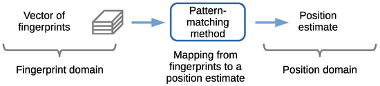
Figure 5.
Fingerprints-to-position mapping using a pattern-matching method.
Many pattern-matching methods and associated algorithms have been developed for estimating a position from a set or vector of fingerprints. Some examples of these are look-up tables [36], databases [37], k-Nearest Neighbors (kNN) [38], fuzzy logic [39], decision trees [40], probabilistic methods [41], genetic algorithms [42], support vector machines (SVMs) [43], and artificial neural networks (NNs). Look-up tables, also known as databases, map a sampled set of fingerprints to a ground truth reference position. These are implemented in the form of tables in databases, matrices, or any suitable data structures and are combined with a given general-purpose algorithm (e.g., a greedy algorithm or least-squares minimization) to estimate the position by finding the closest set of fingerprints that matches a given input. Another way to map a set of fingerprints to a position is to train a suitable model such that it takes a set of fingerprints as the input and returns a set of position coordinates as the output. Ultimately, the goal is to generalize the model that maps the input set of fingerprints to a position estimate such that it returns as its output a position estimate with a statistically minimal positioning error.
An overview of the machine learning methods used in fingerprinting-based positioning and the motivation for using pattern-matching methods based on machine learning is discussed in [44,45,46,47,48].
In fingerprinting-based positioning, the typical use of an FFNN with supervised learning and a regression-based model consists of providing as input to the FFNN a set or vector of N fingerprints from N fingerprint sources. The training is carried out to match labeled data. The labeled data consist of 2D or 3D ground truth position coordinates associated with the input fingerprints.
Then, in the testing phase, an estimate of the position is obtained from the output of the FFNN for a given input set or vector of fingerprints.
In the context of this article, we work only in the Euclidean plane; hence, we use as the positioning error the error distance. The error distance is the Euclidean distance between the ground truth reference position and the estimated position. In 2D, with ground truth position coordinates , and estimated position coordinates , for a set of fingerprints , the error distance, , is
Throughout this article, we use to represent a set of fingerprints. We use the same notation to either represent the set of fingerprints that forms the elements of a vector of fingerprints associated with a position or to represent all of the fingerprints that can form multiple fingerprint vectors, associated with multiple positions.
2.3. Mobile-Device-Based Positioning
In a study centered on radio-network-based localization services [9], a categorization is presented differentiating which is the entity responsible for the position estimation. In one category, a radio mobile device is responsible for the estimation of its own position. In another category, the network is responsible for estimating the position of the radio mobile device. A more concise categorization is used in the standards for cellular radio networks, where the positioning methods are classified into mobile-based (also known as user-based or user-equipment-based), mobile-assisted, network-based, and network-assisted [49,50,51,52].
Similarly, we differentiate between cases in which the position estimate is performed by a communications or positioning infrastructure and by a mobile positioning device. In this context, the positioning device is a mobile entity intended to estimate its own position. Here, these cases are referred to as infrastructure-based positioning, shown in Figure 6a,b, and mobile-device-based positioning, shown in Figure 6c,d,e. In the former, the position estimate is made by the communications or positioning infrastructure. In the latter, the position estimate is made by the mobile positioning device. In the case of fingerprinting-based positioning using radio signals, the infrastructure utilizes fingerprints from uplink signals, whereas mobile devices utilize fingerprints from downlink signals.
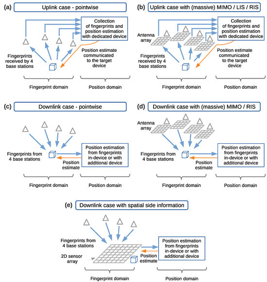
Figure 6.
Differentiation of the position estimate made by the infrastructure (infrastructure-based positioning) in the uplink direction (a,b) and the position estimate made by a mobile positioning device (mobile-device-based positioning) in the downlink direction (c–e). Triangles represent base stations, and cubes represent positioning consumers or positioning devices.
In the infrastructure-based positioning case, the positioning process is carried out in two steps; see Figure 6a. First, the devices transmit radio signals in uplink. Then, the radio signal information is collected as fingerprints in a distributed manner on the infrastructure side from all of the base stations involved, and the position estimate is computed using a dedicated device. Second, the position estimate is communicated to the positioning consumer. In this case, the consumer of the position estimate may not exactly be called the positioning device. In the literature, it is simply called the transmitter, or the positioning tag in some cases, as it is the device that generates the signal toward the infrastructure.
A variation of the infrastructure-based positioning case is shown in Figure 6b, in which arrays of antennas for MIMO, massive MIMO [53], cell-free massive MIMO [54,55,56], Large Intelligent Surfaces (LISs) [57], or reconfigurable intelligent surfaces (RISs) are used at the base stations for positioning purposes, with the mobile users transmitting in uplink. Some examples of fingerprinting-based positioning with uplink transmission are [58,59,60,61,62,63,64,65] for massive MIMO, [66,67] for cell-free massive MIMO, [68] for LISs, and [69,70] for RISs.
In the mobile-device-based positioning case, the device receives the radio signals transmitted in downlink by the infrastructure and collects these as fingerprints; see Figure 6c. Then, the device itself or an additional supporting device estimates the position without further involvement of the infrastructure. A variation of this case is shown in Figure 6d, in which the base stations utilize MIMO, or massive MIMO, antenna arrays for positioning in downlink. In addition, some works propose the use of RISs for the downlink case. Some examples of fingerprinting-based positioning with downlink transmission are [71] for MIMO, [72,73] for massive MIMO, and [74,75] for RISs.
Finally, we present a variation of the mobile-device-based positioning case with the signals in downlink, for the case of fingerprinting-based positioning with spatial side information, in Figure 6e. In this case, the downlink radio signals are received by the 2D sensor array to exploit the spatial side information. The processing of the fingerprints is performed in the device itself or using an additional supporting device.
We do not consider in our scope the infrastructure-based positioning case. This is because in order to minimize the positioning error, this case would require increasing complexity and cost on the positioning infrastructure side, which is not aligned with our objective. In addition, this case relies on network communication, centralizing the fingerprints that are collected at the different nodes or base stations. In some use-cases with limited communication, this may degrade the reliability of the positioning estimates. Hereafter, we focus only on mobile-device-based positioning using downlink radio signals as fingerprints for the case using spatial side information (Figure 6e). This case will be benchmarked against a traditional fingerprinting method operating with downlink radio signals and no side information (Figure 6c).
2.4. Positioning Data Aggregation Domains for Fingerprinting-Based Positioning
As was introduced in Section 2.2 and depicted in Figure 5, the pattern-matching method maps an input set of fingerprints to a position estimate. Here, fingerprints are assumed to belong to a fingerprint domain (also referred to as the signal space in the literature [76]) and positions to a position domain. In this context, the availability of multiple sets of fingerprints associated with a position could be handled either in the fingerprint domain, before the input to the pattern-matching method, or, alternatively, in the position domain at the output of the pattern-matching method. In this last case, fingerprints are input into the pattern-matching method individually, one set or vector at a time, resulting in one output position estimate for each input set of fingerprints. So, because the ultimate goal is to estimate one final position, the availability of multiple position estimates associated with a position must be handled in the position domain to produce a final position estimate.
As a reference, the most commonly observed approach in the literature consists of feeding multiple sets of fingerprint samples into a pattern-matching method to obtain multiple position estimates, with each one associated with an input set of fingerprints. Then, the multiple position estimates are aggregated in the position domain. In the case of multiple position estimates for a fixed position, the usual approach to obtaining a final position estimate is to aggregate the multiple position estimates through averaging. In the case of multiple position estimates being obtained through the movement of a positioning device along a path, the usual approach is to aggregate the multiple position estimates by relaying on a filter that smooths the past position estimates in the position domain.
The actual aggregation of the fingerprint data, before their input into the pattern-matching method, in the fingerprint domain is usually carried out by averaging the fingerprints. In this case, multiple sets of fingerprints are aggregated into a single set; thus, any additional information that could be obtained from the complete set is removed and lost. The actual exploitation of the information contained in multiple sets of fingerprints has received less attention in the literature, although this was found in a few articles (discussed in Section 3.2).
In the articles surveyed (Section 3), we did not observe classification of or differentiation between the positioning data domains for the fingerprints and positions. Because some of our pattern-matching methods work in one domain or the other, we need to make this distinction by introducing the classification of the cases listed in Table 2. The cases listed in the table are based on the input to, and output from, the pattern-matching method and based on the positioning data aggregation domains.
Table 2.
Cases for pattern-matching method and positioning data aggregation domains.
The three cases of pattern-matching methods and positioning data aggregation domains listed in Table 2 are associated with the three cases depicted in Figure 7. These cases are explained next.
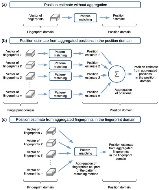
Figure 7.
Cases for pattern-matching methods and positioning data aggregation domains. (a) Position estimate without positioning data aggregation. (b) Position estimate from aggregated positions in the position domain. (c) Position estimate from aggregated fingerprints in the fingerprint domain.
2.4.1. Position Estimates Without Positioning Data Aggregation
Case 1 (in Table 2), in Figure 7a, consists of pointwise mapping from the fingerprints to a position estimate, in which the pattern-matching method takes as input a set or vector of fingerprints and outputs a position estimate. In this case, there is a direct mapping from the fingerprints to a position estimate, so there is no positioning data aggregation. By pointwise, we refer to a case in which a position is estimated at a single spatial point, through a set or vector of fingerprints, without side information, in a single sensing or receiving element of the positioning device.
2.4.2. Position Estimates from Aggregated Positions in the Position Domain
Case 2 (in Table 2), in Figure 7b, consists of aggregating the positions in the position domain, at the output of n instances of the pattern-matching method, to estimate the position. In this case, a collection of several, say n, sets or vectors of fingerprint samples is presented as the input. Each one of the n fingerprint vectors is individually input into the pattern-matching method to produce an independent position estimate at the output. The pattern-matching method applied to each input can be the same or differ. Here, we will consider the same method implementing the same model for all the inputs. The instances of the pattern-matching method can be processed sequentially or in parallel. The sequential implementation handles one input set or vector of fingerprints at a time. The parallel implementation handles multiple instances of the pattern-matching method to process each one of the input sets or vectors at once. Thus, for a given number of n input vectors of fingerprints, there are n output position estimates. Then, the n position estimates are aggregated in the position domain into a single final position estimate. This aggregation is carried out using a suitable function or operation, for example, the mean value or weighted average, that computes the final position estimate. In the context of the work presented in this article, the n input vectors of fingerprints will be collected simultaneously at adjacent positions by means of the 2D sensor array when the 2D sensor array is in a fixed position in space. However, alternative approaches could be devised for the collection of fingerprints at adjacent positions (as discussed in Section 4.1).
It is noted that in the literature, some authors consider collections of fingerprint vectors that are collected by moving a positioning device along a path. In some cases, each one of the fingerprint vectors is individually mapped to a position, and then a smoothing filter is applied to enhance the estimation of a new position by relying on the past position estimates. While this approach technically uses adjacent side information and also can be classified into this case, this approach is not considered to be within the scope of our work. The reasoning for this is that first, the filtering operates in the position domain, whereas we intend to operate in the fingerprint domain in order to extract as much information as possible from the fingerprints. Second, the usual movement of a positioning device along a path that is considered in the literature has a granularity or resolution that it is coarser than what we aim to obtain with the 2D sensor array. Third, unless the area in which the positioning is intended is comprehensively scanned in a particular way, the usual movement along a path is not suitable for considering side information in 2D. And fourth, the filtering process can be viewed as a weighted average of the adjacent position estimates with either a set of manually assigned weights or a set of weights statistically calculated using a few parameters. Regarding this approach, we argue that an NN with a suitable structure and size can operate as a more tailored model for the problem. Another aspect to consider is that by employing multiple sensors, the proposed approach based on the 2D sensor array will produce position estimates which would be equivalent to the future position estimates in solutions relying on collecting fingerprints by moving a positioning device along a path.
2.4.3. Position Estimates from Aggregated Fingerprints in the Fingerprint Domain
Case 3 (in Table 2), in Figure 7c, consists of aggregating the fingerprints in the fingerprint domain before performing the mapping of the fingerprints to an estimated position through a pattern-matching method. In this case, a collection of several, say n, sets or vectors of fingerprint samples is presented as the input. All of the n fingerprint vectors are aggregated in the fingerprint domain. This aggregation is carried out using a suitable function or operation, built into the pattern-matching method, or in a separate module prior to the pattern matching. In the case of combining the aggregation with the pattern matching, the pattern-matching method is applied simultaneously to the n input fingerprint vectors to produce as the output a position estimate for all of the input vectors. In the case of a pattern-matching method based on an NN, it can be left to the training phase to find a weighted average for the input fingerprints, thus integrating the aggregation as part of the NN model. In contrast, performing the positioning data aggregation in a separate module, may destroy information that otherwise could be used by the NN from the input to the output to produce a better position estimate. Nevertheless, the aggregation can be carried out in a module independent of the pattern-matching method if desired. For example, a common approach applied in field measurements consists of averaging the fingerprints collected in the time domain for a fixed position and then inputting these into the pattern-matching method.
In case number 3 in Table 2 and in Figure 7c, the actual aggregation of fingerprints is assumed to be part of the pattern-matching method, and therefore, it is not explicitly shown.
In the context of the work presented in this article, the n input vectors of fingerprints will be collected simultaneously at adjacent positions by means of the 2D sensor array when the 2D sensor array is at a fixed position in space.
In the literature, some authors consider a collection of fingerprint vectors collected by moving a positioning device along a path. In contrast to the approach discussed in the previous subsection of aggregating the position estimates in the position domain, some authors aggregate the fingerprints collected by moving along a path in the fingerprint domain by considering a time-series of spatially distributed fingerprints. These research works are discussed in Section 3.2.
2.5. Spatial Side Information
In the field of fingerprinting-based positioning, research is focused on how to obtain and extract as much information as possible from the sources generating the fingerprints in the time, space, and frequency domains, in addition to proposing different pattern-matching methods for processing such information. The use of filters to process a time-series of fingerprints can be seen as one of the first attempts to exploit side information in the time domain. When multiple fingerprints are collected at the same static position, increasing the number of samples reinforces the statistics to obtain a better position estimate. When multiple fingerprints are collected in a geographical area by moving a positioning device along a path and when the displacement is slow compared with the sampling rate, it can be assumed that the previous position estimates are closer to the current position. Thus, past position estimates provide side information that can be exploited to estimate the current position in a combination of the time and space domains. Further information from other sources, like inertial sensors, contributes to the local information about the relative distances between samples. Information on the distances between samples provides additional information that helps to enhance the estimation of the position when compared to the assumption of the locality of neighboring samples without the relative distance information mentioned above. This constitutes information from the space domain that it is then associated with the collected fingerprints and processed using a suitable pattern-matching method to further enhance the position estimate. In the space domain, we can also consider different antenna arrangements, as well as a strategic geographical distribution of the fingerprint sources, that helps to incorporate and exploit the side information in the space domain. Finally, the availability of multiple subcarriers from Orthogonal Frequency Division Multiplexing transmissions is exploited to increase the number of amplitude and phase fingerprint sources in the frequency domain. In this article, we focus on 2D side information in the space domain.
We use spatial side information to refer to any information that can be extracted around the target position that we intend to estimate. We call it spatial because the side information has associated a position, relative or not, whether known or estimated, with the target position. In fingerprinting-based positioning, the side information is most likely additional fingerprints collected at physically adjacent positions to the position to be estimated.
The motivation for considering spatial side information lies in exploiting more and correlated information. In the case of using the proposed 2D sensor array, we have additional knowledge on the relative position of one fingerprint sensor or receiver to that of the other ones. We consider this side information analogous to the encoding of information in a transmitter of a generic communications system, in which adjacent bits are related to each other by means of an encoder implementing a code such as a convolutional or turbo code [77,78]. As in a communications system, we expect to obtain a gain from the use of side information, making the pattern-matching method more robust to the variations in the RSS fingerprints.
Spatial side information can be obtained either (1) by one sensor sampling fingerprints in the time domain, with a known or estimated relative movement around the target position, or (2) through simultaneous sampling of the fingerprints with an arrangement of multiple sensors, like in an array or matrix arrangement, in which the relative position of each sensor is known. In this study, we consider the latter case, with a 2D sensor array simultaneously sampling multiple fingerprints around the position to be estimated.
The typical case found in the literature is case (1) cited above. In this case, one receiver or sensor from a positioning device collects a set of fingerprints at one position, and then it is moved to a neighboring or adjacent position to collect another set of fingerprints. The set of fingerprints is mapped to a position estimate at each sampled position using a selected pattern-matching method. This process may be repeated for a certain number of positions or indefinitely. Finally, the current position is estimated using a filter (e.g., a smoothing filter), relying on the past position estimates. That is, each target position estimate is the result of the mapping of a set of fingerprints associated with the target position, plus the past position estimates. Certainly, this approach uses spatial side information to estimate a position. However, we argue that such an approach to estimating a position is the result of the aggregation of the past position estimates in the position domain, as depicted in Figure 7b, and not in the fingerprint domain, as depicted in Figure 7c.
Here, we are interested in using the fingerprints from the target, as well as from adjacent spatial positions, entirely in the fingerprint domain, that is, before the fingerprints from the target and adjacent positions are mapped to a target position estimate. At the end of this article, we will benchmark a pattern-matching method operating in the position domain against two pattern-matching methods operating in the fingerprint domain and draw conclusions from the results obtained.
2.6. Data Aggregation Domains, Side Information, and Analogy to Communications Systems
We are interested in exploiting spatial side information in the fingerprint domain before mapping the fingerprints to an estimated position. It is argued that aggregating the positions in the position domain will result in accumulating the errors introduced by the pattern-matching method for each position estimate in the aggregation stage. In contrast, aggregating the fingerprints in the fingerprint domain would result in processing raw data, with more information, before calculating the position estimates using the patternmatching method.
The reasoning stated above is analogous to the estimation of transmitted bits in a communications system, using so-called hard-bits and soft-bits (as a result of implementing hard-decision or soft-decision decoding) [77,78].
Let us focus for a while on the receiver side of a communications system implementing digital amplitude modulation. As one possibility, the receiver can work with hard-bits. Hard-bits result from quantizing analog information in the demodulator from each received symbol into bits with ultimately one of two possible states (0 or 1). Assuming that the transmitted bits are encoded, these hard-bits are then post-processed in a decoding stage to obtain an estimation of the transmitted bits. With this approach, the quantization removes information that otherwise would have helped the decoder to reduce the decoding error and to ultimately produce a better estimate of the transmitted bits.
Alternatively, the receiver can work in the decoding stage with raw information or soft-bits, that is, analog information from each received bit expressed as a real number, prior to the quantization stage. This last approach is beneficial for retaining as much information as possible from the received symbols or bits during the decoding phase. It is particularly implemented with error correction codes designed to exploit information from adjacent bits, such as convolutional codes or turbo codes, and complemented with a suitable decoder that makes use of this side information. The decoder ultimately outputs the estimated transmitted bits as real numbers for posterior quantization.
Now, we can make an analogy in which the pattern-matching method in our positioning system would be analogous to the quantizer of a receiver, and the aggregation of data (fingerprints or positions) in our positioning system would be analogous to what occurs in the decoder of a receiver (Figure 8).
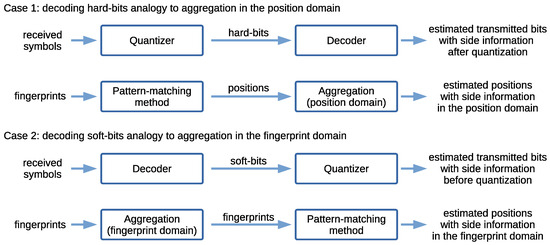
Figure 8.
Data aggregation domains, side information, and analogy to communications systems.
More specifically, the first case (hard-bits), depicted as Case 1 in Figure 8, associates the following analogies. A quantizer (or a demodulator fulfilling this function) quantizing the received bits or symbols into hard-bits (without exploiting the side information) is analogous to a pattern-matching method estimating the positions without exploiting side information. A decoder working with hard-bits is analogous to posterior aggregation, in the position domain, of the estimated positions output by the pattern-matching-method to produce a final position estimate. Then, the second case (soft-bits), depicted as Case 2 in Figure 8, associates the following analogies. A decoder exploiting the side information from soft-bits (from the received symbols) is analogous to the aggregation of the fingerprints in the fingerprint domain. A quantizer quantizing (or, more specifically, rounding to 0 or 1 at this stage) decoded soft-bits into hard-bits is analogous to a pattern-matching method estimating the positions with the side information in the fingerprint domain.
It is shown later that aggregating the side information in the fingerprint domain results in a better performance in terms of minimizing the positioning error than aggregating independent position estimates in the position domain.
2.7. Summary of the Key Assumptions and Scope
The assumptions and scope of our research are summarized below.
- We focus on fingerprinting-based positioning, with downlink transmission of the fingerprints and fingerprints processing on the positioning device side in 2D.
- The spatial side information on adjacent fingerprints at the positioning device is considered.
- The position is estimated considering positioning data aggregation in the position domain in one of the pattern-matching methods proposed and in the fingerprint domain in two of the pattern-matching methods proposed. However, our main interest is processing the fingerprints in the fingerprint domain before their input into the pattern-matching method.
- The collection of the fingerprints is assumed to be carried out using a two-dimensional sensor array (2D sensor array).
- The same 2D sensor array is used in the training and testing phases.
- An actual description of how the 2D sensor array should be built it is out of our scope. Each sensor, in charge of sampling fingerprints, may be an antenna or a receiver with a built-in antenna. Thus, it may be composed of an antenna array or a receiver array. We do not consider the actual antenna design aspects related to the construction of the 2D sensor array. In this context, we work only with the numeric modules of what would be the equivalent of the received signal strength, ignoring the effects of the constructive/destructive phases of the radio-waves, the optimal antenna spacing, the effect on the antenna spacing and the Signal-to-Noise Ratio (SNR), and variable Angles of Arrival (AoAs) of the radio-waves with respect to the 2D sensor array’s position.
- We carry out positioning in 2D.
- We assume that the fingerprint source nodes (transmitters) belong to the positioning system infrastructure, are always present, and are located in stationary positions.
- It is assumed that the fingerprints are always collected in the same plane, at the same height. In practice, this assumption is not unrealistic considering that the 2D sensor array may not be suitable as a hand-held positioning device. This requirement could be satisfied in practice by mounting the 2D sensor array onto a trolley, robot, or machine operating at the same height.
- Perfect alignment of the 2D sensor array with the positioning area in the scenario considered will be assumed. Rotation and tilting of the 2D sensor array were not considered in our study.
- It is assumed that a subdivision of the tile (called a sub-tile) is the smallest granularity for discretizing the positioning area and the sample positions. These subdivisions are non-overlapping, of a square shape, and uniform in size.
- We utilize Monte Carlo methods to generate synthetic RSS fingerprints. We will assume an omnidirectional radiation pattern for the antennas of the transmitters, an LOS radio propagation channel model, and transmitters with a constant transmit power.
- The primary goal is to observe whether using the spatial side information on the RSS fingerprints by means of an ideal 2D sensor array produces any gain in terms of minimizing the positioning error.
- It is out of the scope of this article to evaluate the computing cost of the patternmatching methods proposed.
- It is not part of our claim that the use of pattern-matching methods based on feedforward and convolutional NNs will outperform any other method. These were selected, and used as a tool, based on the general performance of these in the fields of fingerprinting-based positioning and pattern matching in images. Furthermore, NNs were selected for the proposed pattern-matching methods because among all of the deep learning methods known, NNs possess a competitive learning capacity. Our main goal, as stated, is to observe whether the use of spatial side information brings a gain. If a gain, in terms of minimizing the error distance, is observed with some of the selected methods, future in-depth research on the selection of the most optimal pattern-matching methods can be considered. An initial contribution in this direction is provided by studying the pattern-matching methods proposed and comparing the results produced by them.
3. Literature Review and Related Work
A survey was carried out centered on identifying previous work proposing the use of spatial side information on the device side with downlink transmission (in the case of fingerprints based on radio signals) in 2D and, particularly, aggregating the fingerprints in the fingerprint domain. We aimed to learn the state of the art in this area and to identify whether there is an existing approach equal or similar to that proposed by us.
Research works estimating positions through the aggregation of past position estimates using smoothing filters (e.g., moving average filters, Kalman-based filters [79], etc.) are not considered. These works may exploit spatial side information when the fingerprints are collected by the movement of a positioning device along a path. However, the final position estimate relies on aggregation of the positions in the position domain. In contrast, we are interested in the exploitation of spatial side information in the fingerprint domain before mapping the fingerprints to an estimated position. Another consideration in ruling out works utilizing filters is that typically, the fingerprints collected by the movement of a positioning device along a path have associated side information in only one dimension. Even when the displacement is along a 2D path, the relationship of each neighboring position ultimately contributes to the side information in one dimension. Thus, filtering is typically carried out on position estimates that have side information along one dimension.
Part of our survey was carried out by looking at research works discussing positioning with 2D antenna arrays, (massive) MIMO, LISs, and RISs. However, these works focus mainly on uplink transmissions (see the references in Section 2.3). Actually, LISs and RISs are considered for the downlink case, although not on the device side but as a complementary and static component to enhance the positioning, as discussed, for example, in [80,81,82,83].
We surveyed research works using two particular approaches that could be related to exploiting spatial side information on fingerprints in 2D.
One possible approach to exploiting the side information consists of the use of the convolution operation. Convolution is an operation that relies on the adjacent data, and therefore, it may serve as a keyword for finding works dealing with spatial side information. From a general survey, we identified that in the field of fingerprinting-based positioning, convolution of the fingerprints is generally applied using CNNs. Thus, we surveyed the use of CNNs with fingerprinting-based positioning, focusing particularly on 2D CNNs. A secondary goal of surveying works adopting 2D CNNs was to identify any possible work aligned with our approach, that is, on collecting fingerprints in 2D on the device side, in downlink, and implementing a pattern-matching method based on a 2D CNN to exploit the side information.
A second possible approach to exploiting side information consists of the use of time-series or sequences of spatially distributed fingerprints. A time-series of fingerprints can be generated by moving a positioning device along a path. In this case, the positioning device may implement a single sensor or receiver, as is commonly found in the literature, to sample the fingerprints. Then, sampling the fingerprints during the movement of the positioning device along a path allows spatially distributed fingerprints to be collected. Thus, we surveyed this category to identify the possible use of spatial side information in 2D. It is noted that some research works gather fingerprints in static positions, without movement, to generate time-series of fingerprints. These works do not contain spatial side information as it is considered in the context of our research; therefore, these works are not considered in our survey.
In addition, we surveyed other research works using spatial side information through other methods than those mentioned above. The results of our literature review are summarized in the next subsections.
3.1. Fingerprinting-Based Positioning Implementing Fingerprint Images Processed Using CNNs
A 2D CNN operates with an input of values, in our case fingerprints, arranged into a matrix (or, in a more general case, a tensor). In the literature, in the context of fingerprintingbased positioning, the input matrix is often referred to as a fingerprint image. In the context of our work, the fingerprint image is that produced by the 2D sensor array.
We surveyed research works on fingerprinting-based positioning implementing fingerprint images processed using CNNs in 2D, considering only the case of downlink transmissions in positioning systems based on radio signals. It was out of our scope to study the case of device-free positioning systems, such as that discussed in [84,85,86], on the basis that positioning is not performed at the device and that it was not aligned with our goal of transferring the complexity and costs from the infrastructure to the positioning device. The objective is to identify whether some work proposes the use of spatial side information in 2D through a CNN, on the positioning device side, in downlink, and, preferably, through simultaneous sampling of the fingerprints. The works reviewed are listed in Table 3. In some of these articles, the details of the CNN were not provided. Thus, we inferred the CNN’s structure from the context, e.g., according to the authors’ definition of the fingerprints as the image input to the CNN or the dimensions of the convolution kernel. For more details, refer to the corresponding articles.
The fingerprint images reported in the table are, in most of these cases, found in the context of a 2D image (matrix), which is processed using a 2D CNN in the first layer of the adopted NN structure. The actual input to the CNN may have a third dimension, meaning that a set of images is stacked to form a tensor. In most of these cases, the images that form this third dimension are handled independently at the input of the NN. These images are referred to as channels, in a context analogous to the primary color channels in a color image. In the case of fingerprints based on radio signals, the channels are typically the different sources of the fingerprints, such as access points, base stations, or links in general. In the case of fingerprints from geomagnetic measurements, the channels are typically the coordinates measured using a magnetometer. The main purpose of listing the composition of the fingerprint image for each work surveyed is to identify the possible composition of an image implementing information from two coordinates in space. For details of the actual composition of the input to the CNNs, refer to the corresponding articles.
Our expectation is to find fingerprint images composed of two spatial dimensions and accordingly observe a 2D CNN operating in two dimensions in space. However, at first glance, we observe from this survey that there are two main trends for the creation of fingerprint images, one applied to the case of RSS-based fingerprints and the other applied to the case of CSI-based fingerprints. In the first trend, most of the works adopting RSS fingerprints compose image-like arrangements of fingerprints that do not possess spatial information. These works instead consider a specific arrangement of the fingerprints into a matrix form, usually arranging sub-vectors of a vector of fingerprints as rows in a matrix. In the second trend, that is, in the case of CSI-based fingerprints, in general, the fingerprint images are composed in one dimension of a time domain component and in the other dimension of a frequency domain component. In the case of Orthogonal Frequency Division Multiplexing systems, the frequency domain component consists of the amplitudes or phases of the subcarriers.
Regarding the collection of the fingerprints in the training phase, the works reviewed collect a given number of fingerprint samples at so-called reference positions, also referred to as reference points. The reference positions are either manually or randomly selected in the whole area in which the positioning is intended. The reference positions define the mapping between the fingerprints and the ground truth positions in the training phase. The reference positions are, in some works, set at uniform distances from each other. In some works, the whole positioning area is discretized into small discretized positioning areas or grids, which are treated as reference positions. Discretized positioning areas are explicitly defined as such in the scenario considered or simply defined in general terms as areas, with associated inter-area distances. In some articles, the reference points are provided in the selected dataset. Some examples of the datasets referred to in the surveyed articles are [87,88].
Table 3.
Fingerprinting-based positioning implementing fingerprint images processed using CNNs (downlink case).
Table 3.
Fingerprinting-based positioning implementing fingerprint images processed using CNNs (downlink case).
| Ref. | Year | Fingerprints Used | Discretized Positioning Area Size | CNN Type | Fingerprint Image | Side Inform. |
|---|---|---|---|---|---|---|
| [89] | 2017 | CSI: amplitude | to m | 2D | 30 subcarriers by 30 time samples | (Yes) 3 |
| [90] | 2017 | CSI: AoA | m × path width | 2D | Matrix of AoA values | (Yes) 2 |
| [91] | 2017 | CSI: AoA, amplitude | m × path width | 2D | 30 subcarriers by 30 time samples | (Yes) 3 |
| [92] | 2018 | CSI: amplitude | Ref. points spaced at m | 2D | 30 subcarriers by 30 time samples | (Yes) 3 |
| [93] | 2018 | RSS and correlation coefficient | m m | 2D | Fingerp. arranged in a matrix | No |
| [94] | 2018 | RSS | Building/floor size. | 2D | Fingerp. arranged in a matrix | No |
| [95] | 2018 | RSS | Not specified | 2D | Fingerp. arranged in a matrix | No |
| [96] | 2018 | RSS | Building/floor (classification) | 2D | Fingerp. arranged in a matrix | No |
| [97] | 2018 | CSI | m m | 2D | From CSI wavelet transform | (Yes) 3 |
| [98] | 2019 | RSS | Ref. points spaced at m | 2D | Fingerp. arranged in a matrix | No |
| [99] | 2019 | RSS and kurtosis from RSS | m m and m m | 2D | 3D tensor (number of access points × time × fingerprint and kurtosis) | No |
| [100] | 2019 | RSS | m mean dist., outdoor | 2D | Fingerp. arranged in a matrix | No |
| [101] | 2019 | RSS | m m | 2D | Fingerp. arranged in a matrix | No |
| [102] | 2019 | RSS | m m | 2D | Fingerp. arranged in a matrix | No |
| [103] | 2019 | CSI: amplitude | m m | 2D | 90 subcarriers by 90 time samples | (Yes) 3 |
| [104] | 2019 | RSS with wavelet transform | m m (corridor of m divided into 21 areas) | 2D | 2D representation of RSS via wavelet transform | No |
| [105] | 2019 | RSS | m m | 2D | Fingerp. arranged in a matrix | No |
| [106] | 2019 | CSI: amplitude, phase difference | Ref. points spaced at m | 2D | 114 subcarriers by 114 time samples | (Yes) 3 |
| [107] | 2019 | CSI: amplit., phase | Ref. points from to m | 3D | Fingerp. arranged in a tensor | (Yes) 3 |
| [108] | 2019 | CSI | Ref. points spaced at m | 2D | Channel state matrix | (Yes) 3 |
| [109] | 2019 | Radio beams | From dataset; see [109] | 2D | Number of beams by time samples | (Yes) - |
| [30] | 2020 | Geomagnetic | m m | 2D | Fingerp. arranged in a matrix | No |
| [31] | 2020 | Geomagnetic | Room size | 2D | Fourier transform of fingerprints arranged in a matrix | No |
| [110] | 2020 | CSI: AoA | m × path width | 2D | 60 subcarriers by 60 time samples | (Yes) 3 |
| [111] | 2020 | CSI: amplitude, phase difference | to m | 2D | 30 subcarriers by 50 time samples | (Yes) 3 |
| [112] | 2020 | CSI: amplitude, phase | m m | 2D | Fingerp. arranged in a matrix of 30 subcarriers by 30 time samples | (Yes) 3 |
| [113] | 2020 | RSS and other | Reference points spaced on average from m to m | 2D | Fingerp. arranged in a matrix of the topology of the access points | No |
| [114] | 2020 | CSI: amplitude | Ref. points spaced at m | 2D | Fingerp. arranged in a matrix | (Yes) 3 |
| [115] | 2020 | RSS | m m | 2D | Fingerp. arranged in a matrix | No |
| [116] | 2020 | RSS | m m | 2D | Fingerp. arranged in a matrix | No |
| [117] | 2020 | RSS | 25 m m to 200 m m | 2D | Fingerp. arranged in a matrix | No |
| [118] | 2020 | RSS | to m [88] | 2D | Fingerp. arranged in a matrix | No |
| [119] | 2020 | RSS | m m | 2D | Fingerp. arranged in a matrix | No |
| [120] | 2020 | SNR | m m | 2D | Beam covariance matrix | Yes 32 |
| [121] | 2020 | Radio beams | From dataset; see [121] | 2D | Number of beams by time samples | (Yes) - |
| [122] | 2020 | Radio beams | From dataset; see [122] | 2D | Number of beams by time samples | (Yes) - |
| [123] | 2021 | CSI: amplitude differences | m m, m m, and m m | 2D | Fingerp. arranged in a matrix of 30 subcarriers by 30 time samples | (Yes) 3 |
| [124] | 2021 | RSS | m mean dist., outdoor | 2D | Fingerp. arranged in a matrix | No |
| [125] | 2021 | RSS | Bounding box with estimated position in 40 m m area | 2D | Fingerp. arranged in a matrix | No |
| [126] | 2021 | RSS | Not specified | 2D | Fingerp. arranged in a matrix | No |
| [127] | 2021 | RSS and phase difference | m m | 2D | Fingerp. arranged in a matrix | No |
| [128] | 2021 | CSI | m m | 2D | Amplitude feature map | (Yes) 3 |
| [129] | 2021 | CSI: AoA, amplitude | m × path width | 2D | 30 subcarriers by 30 time samples | (Yes) 3 |
| [130] | 2021 | Geomagnetic | Not specified | 2D | Sequence of fingerprints arranged in a matrix | Yes 700 |
| [131] | 2021 | Geomagnetic | m m | 2D | Sequence of fingerprints arranged in a matrix | Yes 10 |
| [132] | 2021 | RSS | Ref. points spaced between m and m | 2D | Fingerp. arranged in a matrix sorted by the spatial relationship of the access points | No |
| [133] | 2021 | CSI: amplitude | Not specified | 2D | Fingerp. arranged in a sub-window | Yes 16 |
| [134] | 2021 | RSS | m m, m m | 2D | Matrix of scaled diff. of fingerp. | No |
| [135] | 2021 | CSI: amplitude | Not specified | 2D | 30 subcarriers by 30 time samples | (Yes) 3 |
| [136] | 2021 | RSS | m m | 2D | Fingerp. arranged in a matrix | No |
| [137] | 2021 | RSS | Ref. points spaced at m | 2D | Fingerp. arranged in a matrix of the topology of the access points | No |
| [138] | 2022 | RSS | Ref. points spaced at m | 2D | Fingerp. arranged in a matrix of time and frequency | No |
| [139] | 2022 | RSS | m m to m m | 2D | Fingerp. arranged in a matrix of the topology of the access points | No |
| [140] | 2022 | CSI: phase | m m | 2D | 30 subcarriers by 30 time samples | (Yes) 3 |
| [141] | 2022 | CSI: amplitude | m m | 2D | 30 subcarriers by 200 time samples | No |
| [142] | 2022 | RSS and other | m m | 2D | Four measurements by time sampl. | No |
| [143] | 2022 | RSS | m m | 2D | Matrix of vertical–horizontal beams | No |
| [144] | 2022 | RSS | to m [88] | 2D | Fingerp. arranged in a matrix | No |
| [145] | 2022 | RSS | According to [87] | 2D | Fingerp. arranged in a matrix | No |
| [146] | 2022 | RSS | m m | 2D | Fingerp. arranged in a matrix | No |
| [147] | 2022 | RSS | Ref. points spaced m | 2D | From a rasterization function | No |
| [148] | 2022 | CSI | Ref. points at or m | 2D | 30 subcarriers by 36 time samples | (Yes) 3 |
| [149] | 2022 | RSS | m m | 2D | Vector of fingerp. sampled in time arranged as a matrix | No |
| [150] | 2022 | RSS | Ref. points spaced at m | 2D | Fingerp. arranged in a matrix | No |
| [151] | 2022 | CSI | Ref. points at approx. m | 2D | Not specified | No |
| [152] | 2022 | RSS | According to [87] | 2D | Fingerp. arranged in a matrix | No |
| [153] | 2022 | RSS | m m | 2D | Vector of fingerp. sampled in time and space arranged as a matrix | Yes 40 |
| [154] | 2022 | RSS | to m [88] | 2D | Fingerp. arranged in a matrix | Yes 2 |
| [155] | 2022 | RSS | to m [88] | 2D | Fingerp. arranged in a matrix | No |
| [156] | 2022 | RSS | m m | 2D | Vector of fingerp. sampled in time arranged as a matrix | No |
| [157] | 2023 | CSI: amplitude | Ref. points spaced at m | 2D | 256 subcarriers by 1000 time sampl. | No |
| [158] | 2023 | RSS | m m | 2D | Vector of fingerp. sampled in time arranged as a matrix | No |
| [159] | 2023 | RSS | Ref. points spaced at m | 2D | Matrix of row vectors of fingerp. | No |
| [160] | 2023 | RSS | Not specified | 2D | Fingerp. arranged in a matrix of the vertical–horizontal topology of the access points | No |
| [161] | 2023 | CSI: amplitude | Ref. points spaced at m | 2D | 60 subcarriers by 60 time samples | (Yes) 3 |
| [162] | 2023 | CSI: amplitude | m m | 2D | 30 subcarriers by 30 time samples | (Yes) 3 |
| [163] | 2023 | RSS | m m | 2D | Fingerp. arranged in a matrix | No |
The discretized positioning area sizes or equivalent area sizes assumed from the given reference points for each article surveyed are listed in the table. These were reviewed in order to obtain an insight into the granularity or resolution of the discretized positioning area sizes used in the different scenarios and later compare them to the area sizes considered in our proposal. The smallest discretized area size observed in the articles surveyed was m × m. As will be explained in subsequent sections, we explore the use of different discretization area sizes, as determined by the size of the 2D sensor array, starting from m × m.
In the last column of Table 3, we indicate with Yes or No whether the corresponding work used spatial side information or not, respectively. A number after a Yes entry indicates the maximum number of spatial points with side information associated with the fingerprints when this number was stated in the article.
Some entries in the last column of Table 3 are marked in parentheses as (Yes). These correspond to cases in which spatial side information is used in a positioning system based on radio signals, utilizing more than one antenna at the receiver, and differentiating between the fingerprints from each antenna. In these works, we did not observe the use of 2D spatial side information. In general, the antennas were either arranged as a linear array or there was no concrete information stating that a 2D antenna arrangement was used. Therefore, the spatial side information that can be extracted from such antenna arrangements is considered to be side information in 1D. From all the works consulted using multiple antennas at the receiver, only a few have studied the possible gains and effects caused by varying the number of receiving antennas or, in the context of this research, the number of spatial side information points, namely [140,148]. In these articles, it is observed that the larger the number of receiving antennas and thus side information points, the lower the positioning error.
Articles labeled with Yes, without parentheses, in the last column of Table 3 correspond to articles proposing the use of spatial side information on the positioning device side and implementing a 2D CNN. These articles depart from simply using a receiver with multiple antennas, as is the case for entries labeled with (Yes), and therefore need to be differentiated. Each one of these articles are discussed in detail next. We note that, from our perspective, two of the entries labeled with Yes make use of spatial side information in 2D, namely [120] and [133].
In [120], a transmitter and a receiver implementing a 32-element planar antenna array are tested for positioning in the 60 GHz frequency range. The receiver composes a beam covariance matrix from 36 beam patterns, which is processed as a fingerprint image using a 2D CNN. The authors discuss the beam patterns over the azimuth and elevation angles, suggesting the possibility of positioning in 2D in a vertical plane.
In [130,131], geomagnetic fingerprints are collected by walking along a path. Geomagnetic fingerprints are differentiated in 3D using a magnetometer, thus producing three sequences, with one for each dimension. In [130], each sequence is arranged into a square matrix and converted into an image representation. Three images, with one for each dimension, are stacked to form a tensor, which is interpreted as a single image with three channels. This final image is input into a 2D CNN. In [131], each sequence is transformed into a square matrix through a recurrence plot transformation. The resulting matrices from the three dimensions are stacked to form a tensor, which is input into a 2D CNN. In both cases, if there is spatial side information in 2D, it is not preserved in relation to the displacements in 2D. Then, the sequences have adjacent side information relative to the previous and next position, which are interpreted as contributions that are projected into only one dimension.
In [133], the authors propose dividing the whole positioning area into a grid of squares. Each square has a vector of CSI amplitudes associated with it. The authors collect fingerprints by moving in the scenario for a finite number of steps, associated with a sliding window. The fingerprints are then arranged into a so-called sub-window, which is actually a 2D portion of the grid that covers the whole positioning area. Thus, the arrangement of the fingerprints seems to take into account the correlation of the CSI of the neighbor grid squares in 2D. The proposed method exploits these correlations to produce a better position estimate than that which would be obtained without this side information. The positioning resolution is in the order of the size of the squares in the grid.
In [153], RSS fingerprints are collected as a time-series of spatially distributed fingerprints of 5 to 40 time samples by moving a positioning device along a path. The fingerprints at each time sample are arranged as vectors. Then, the vectors for all of the time samples are arranged into a matrix. The matrix is then interpreted as an image and processed using a 2D CNN. In [154], the RSS fingerprints measured at the current and previous position are considered. The fingerprints in these two positions are used as the input in the training and testing phases. Vectors of the RSSs for the current and previous position are arranged as matrices and then converted into images to be processed using a 2D CNN. In the model proposed, each image is first pre-processed by a series of 2D convolution layers and then processed by a layer concatenating the two sources to finally produce a position estimate. From one perspective, this arrangement could be interpreted as a time-series of fingerprints with only two samples. The way to collect and arrange the fingerprints in these two works can be interpreted as the use of a 2D sensor array with a number of sensors equivalent to the number of time steps in [153] and with two sensors in [154]. However, if there is spatial side information in 2D, it is not preserved in relation to the displacements in 2D; that is, the 2D side information does not remain associated with the fingerprints collected. Thus, the fingerprints only have a spatial association with the contiguous ones in 1D as a result of collecting these by moving the positioning device along a path. Therefore, the adjacent side information in these two works is interpreted as 1D side information.
Finally, it is worth mentioning that we identified two articles considering the spatial information in 2D of the access points generating the fingerprints. These articles were labeled as not containing side information in the table because from the perspective of our work, we are trying to identify the use of spatial side information for the fingerprints on the device side. In [139], the fingerprints are arranged into a matrix consistent with the topology of the access points, preserving the spatial relationship of the sources generating the fingerprints. The spatial relationship described in [139] differs from the spatial side information on the device side that we consider in this article. In [160], a matrix of fingerprints is composed in which the rows represent floors. The elements in a row hold the RSS values of a relative projection of the position of the access points on that floor. Thus, the columns in the matrix associate the access points in the same vertical projection.
To summarize our survey of this category, we identified the use of 2D side information in [120] through the use of a 32-element planar antenna array and in [133] through the sampling of a 2D portion of the grid that covers the whole positioning area. We could not find any work that proposed the collection of fingerprints in 2D and the implementation of a 2D CNN as a pattern-matching method, as we propose in our work.
3.2. Positioning Implementing Time-Series of Spatially Distributed Fingerprints
We surveyed research works on fingerprinting-based positioning implementing time-series of spatially distributed fingerprints. The works reviewed are listed in Table 4. In all of the works consulted, the fingerprints are collected with the use of a single sensor or receiver by moving a positioning device along a path, also referred to as a trajectory or route in different works.
Table 4.
Fingerprinting-based positioning implementing time-series of spatially distributed fingerprints (downlink case).
It is noted that the application of machine learning methods to the processing of the time-series of fingerprints implies that the fingerprints are aggregated in the fingerprint domain, as discussed in Section 2.4.
For the processing of the time-series, the literature surveyed adopts 1D CNNs; recurrent neural networks (RNNs); and Long Short-Term Memory (LSTM) NNs [197,198].
RNNs and LSTM NNs are suitable for identifying the long-term dependencies of the time-series. In the context of this work, the temporal structure stored by the RNNs and LSTM NNs can be used to map a relationship between spatially distributed fingerprints and the target position to be estimated. In this case, the time domain is related to the space domain through the collection of the fingerprints, which consists of taking consecutive samples using a positioning device that is moved along a path. For example, in [172] a sequence-to-sequence prediction model is presented. The model takes as its input side information from a sequence of fingerprints collected along a trajectory. As the output, it produces a sequence of position estimates associated with the input.
Moving a single sensor or receiver along a path to gather fingerprints, without additional information on the local displacement, yields as its result a time-series of fingerprints with spatial relationships only between consecutive and adjacent samples. As discussed in the previous subsection, these time-series of fingerprints are interpreted as occurring along one dimension, even when the path described can be in two dimensions. As far as we observe in the works surveyed, if the path is described in 2D, the information about the displacements in 2D does not remain associated with the fingerprints collected, and it is not passed along or preserved to further contribute as side information in 2D. Thus, the time-series only relates the side information from contiguous samples, which is interpreted as side information in one dimension. The last column in Table 4 indicates the number of side information dimensions considered in the works surveyed. We found that in all of the works surveyed, the number of side information dimensions was one; thus, all are labeled as one-dimensional (1D).
A methodology for generating a time-series of fingerprints with spatial side information in more than one dimension is possible, although one was not found in our literature review for this category. One option would be to combine multiple scans along multiple paths to associate adjacent positions in 2D with the target position to be estimated. Relating multiple paths would require the input of additional information from another source, such as from an inertial sensor, to be able to relate the relative displacement between the paths. An example of such an approach is discussed in [199] (details given in Section 3.3). Another option would be to use two or more sensors or receivers such that these were not aligned with the direction of movement along the path. Such arrangements were not found in the literature surveyed. The proposal to use an arrangement of sensing elements as we propose with the 2D sensor array was not found in the literature either.
3.3. Other Works Using Spatial Side Information
In [200], RSS fingerprinting-based positioning is discussed, implemented using a CNN and an input image which preserves the topology of the access points in 2D. The approach proposed in [200] is related to our work through the use of spatial side information; however, it is considered for the access points generating the fingerprints.
In [201], spatial side information is used to generate position coordinates along a path, navigating from a previously created map of clusters, with pre-calculated transition probabilities. Each position’s coordinates on the path generated have an RSS fingerprint associated with them, thus defining a time-series of fingerprints. The time-series of fingerprints is used to train an LSTM NN to estimate the position coordinates for the input path provided.
In [202], a circular antenna array operating in downlink is mounted into a vehicle for 2D positioning. Fingerprinting is performed through a downlink azimuthal-delay representation of the wireless channel.
In [199], RSS fingerprints are collected by moving a positioning device along a path using a hybrid positioning system. The collection of the fingerprints is assisted by side information from an accelerometer and a gyroscope. This auxiliary system provides side information in 2D about the traveled distance and direction. When the trajectory followed is in 2D, the area covered is a small portion of the whole positioning area. Then, a matrix of fingerprints is associated with this small area. The elements in the matrix are associated with the discretization of the small area in the form of a 2D grid of 1 m m squares. The approach proposed in [199] is aligned with ours in terms of gathering fingerprints in 2D; however, it differs in the collection method. In [199], the fingerprints are collected sequentially, with a granularity of 1 m, and in some cases following trajectories that cannot gather side information in 2D. The pattern-matching method proposed is based on finding the best correlation of the measured fingerprints to the stored in a radio map.
In general, we may think that any implementation using a receiver with more than one antenna can be repurposed to exploit spatial side information if independent fingerprints can be extracted from each antenna. So, from one perspective, any receiver with an antenna array can be viewed as a simplified example of the proposed 2D sensor array. However, in the literature reviewed for the downlink case, either (1) linear arrays are considered, suggesting the use of spatial side information in 1D, as, for example, conducted in [203,204] and the other works listed in Table 3, or (2) the geometry of the antenna array is not discussed. Furthermore, the antenna arrays used or proposed for positioning in the literature are not benchmarked against a different antenna arrangement or type to evaluate how different antenna arrangements affect the positioning performance.
3.4. Discussion on Research Works Using Spatial Side Information
We reviewed research works that could make use of spatial side information on the device side in 2D, focusing on downlink transmission for the case of fingerprints based on radio signals. From our survey related to 2D CNNs, we identified the use of 2D side information in [120,133]. From our survey related to time-series of spatially distributed fingerprints, we could not find any research work reporting the use of spatial side information in 2D. From other works, we identified the collection of fingerprints in 2D from portions of the positioning area in [199] and the use of a circular antenna array for 2D positioning in [202]. The above cited works are those with the closest relationship to the approach that we describe in this article; however, these differ in a number of key points. These articles differ in the concept of how to exploit the side information in 2D, in not exploring the possibility of using 2D side information for the creation of a fingerprint image, and in not exploring the possibility of processing the 2D side information using a 2D CNN. Some articles also differ in not simultaneously sampling fingerprints.
In contrast, there are several works making use of spatial side information in 1D by moving a sensor or receiver along a path or trajectory and handling the fingerprints as a time-series. These approaches have in common with our proposal the use of spatial side information, differing, however, by considering only one dimension. Another difference is the sequential sampling of the fingerprints. With the proposed 2D sensor array, multiple adjacent positions are sampled in parallel.
We could imagine that between the use of a moving sensor and the use of the proposed 2D sensor array, a hybrid approach could be devised. This would consist of combining the movement of more than one sensor or receiver along a path. In this hybrid approach, a linear array of sensors or a linear antenna array, aligned perpendicularly with the moving direction, would be moved to generate a matrix of fingerprints analogous to those obtained by the 2D sensor array. Such an approach was not found in the literature. Considerations for this case are outside of the scope in our work.
Many works have composed a so-called fingerprint map or image and handled it as a picture image using a 2D CNN. Our intention was to try to identify whether any research work has proposed composing an image of fingerprints with spatial side information in 2D on the device side. We could not identify such an approach.
As a general summary from our literature review, we could not find any work discussing spatial side information in two dimensions, on the receiver side, and with downlink transmissions for fingerprinting-based positioning. Nor could we find in the literature any proposals related to the utilization of multiple sensors on the positioning device side for the simultaneous sampling of fingerprints in 2D, analogous to the proposed 2D sensor array, for downlink transmissions (in contrast, for uplink transmissions, there are proposals to arrange the antennas into 2D planar arrays on the base station side [205,206]). Then, possibly as a result of there not being a proposal like ours related to the collection of fingerprints in 2D, we did not find any proposals suggesting the construction of fingerprint images in two dimensions. It follows that there was no proposal to implement a 2D CNN as a pattern-matching method exploiting the 2D side information from such fingerprint images.
3.5. Positioning with Discretization of the Positioning Areas and Classification-Based Models
The following research works are related to our work in terms of the discretization of the positioning area and the use of a classification-based model to estimate the positions.
In [73], the positioning area is discretized into different classes. The position is estimated through classification, through a weighted average of the probability for each class and the associated position for each class.
In [207], CSI features are proposed as fingerprints for the uplink case. The positioning area is discretized into so-called grid points. An NN with a softmax output layer estimates the likelihood probability for the users for each grid point, arranged into a so-called probability map. The probability maps are fused across multiple access points to estimate the position of the users.
In [208], the authors discretize the positioning area in an indirect way by assigning a class to a number of reference points distributed across the positioning area. An FFNN with a softmax output layer is trained to map an input vector of fingerprints to a one-hot-encoded vector associated with the class of the reference point where the measurement of the fingerprints is performed. In the testing phase, fingerprints are collected at an arbitrary position. Then, the softmax layer outputs the likelihood probability for each reference point. By relying on the tabulated relationship of each reference point to its coordinates, the position is estimated using the weighted average of the likelihood probability of the class multiplied by the reference position. In addition, the past position estimates are aggregated in the position domain with the current position estimate through a weighted average, influenced by a component from the fingerprint domain given by the similarity of the current vector of fingerprints to past ones.
Other works propose dividing the positioning area into grids and implementing a classification-based model to estimate the positions associated with these grids [120,150,193].
4. Fingerprinting-Based Positioning with Spatial Side Information
In this section, we discuss fingerprinting-based positioning with spatial side information. First, we elaborate on the 2D sensor array and then, in association with this, explain the discretization process in the area fractions with tiles of the area in which the positioning is intended. Next, we describe the positioning process. Finally, we introduce the four pattern-matching methods selected for our study.
4.1. Two-Dimensional Sensor Array
We propose using a two-dimensional array arrangement of sensors, suitable for measuring fingerprints that are physically adjacent in space, as shown in Figure 2. A 2D sensor array makes it possible to collect fingerprints with spatial side information as desired. A set or vector of fingerprints is collected at each sensor in the 2D sensor array.
We formulate a conjecture based on the idea that upon increasing the number of spatial points at which the fingerprints are measured, the amount of information should increase, and therefore, a better estimate of the position should be achieved. This conjecture will be studied through simulations in the following sections.
An actual description of how the 2D sensor array should be built it is out of our scope. The goal is to test whether there is an improvement in the positioning performance, in terms of reducing the positioning error, given the assumption that the 2D sensor array exists.
In this work, we focus on fingerprints based on the signal strengths of radio signals. Therefore, this 2D sensor array could be either a 2D arrangement of multiple antennas with the suitable complementing hardware or a 2D arrangement of multiple independent receivers or sensor nodes.
Also, an arrangement that produces the same output could be devised, for example, by physically scanning using one sensor the area equivalent to that of the 2D sensor array. An alternative approach could combine the movement of more than one sensor to generate a matrix of fingerprints analogous to that obtained by the 2D sensor array—for example, a linear array of sensors or a linear antenna array arranged perpendicular to the direction of movement. In the context of our work, we assume the availability of a 2D sensor array that instantaneously returns the RSS values for each sensor or array element.
The proposal of such a 2D sensor array is not far from the current state-of-the-art. Arrays of multiple antennas are currently in use with massive MIMO technology [53], with the antennas generally arranged into 1D linear arrays. Instead of the typical 1D linear array used in MIMO, in full-dimension MIMO, also known as 3D MIMO, it it proposed for the antennas to be arranged into 2D planar arrays [205,206]. For example, a planar array of antennas, with half-wavelength spacing, for a carrier frequency of GHz would have a size of approximately 462 mm × 462 mm. From the perspective of our study, the challenge is that these antenna arrays have mainly been considered on the base station side of the wireless network. In contrast, our proposal requires such an array of antennas on the positioning device side.
Research on urban navigation utilizing a circular antenna array mounted into a vehicle is reported in [202]. The use of such an antenna array is aligned with the proposed implementation of a 2D sensor array on the device side, although in this case, it is implemented using a circular antenna array.
Intuitively, one may expect that the bigger the sensor array, with more sensors and thus more side information, the smaller the positioning error. The main concern is that the size of such a 2D sensor array should be suitable for real practical use. Possibly, a 2D sensor array with the characteristics required for positioning with spatial side information would not be suitable for use as a hand-held positioning device. However, it should have a size suitable for industrial applications—for example, with a size in the order of that of industrial robots, warehouse trolleys, and moving (autonomous) machinery. Thus, we aim for a 2D sensor array with an approximate side length possibly ranging from 300 mm to 1000 mm.
4.2. Discretized Area Fractions with Tiles
The fingerprint samples measured using the 2D sensor array correspond to the sampling of a small area equivalent to the size of the 2D sensor array. Thus, each sample returned by the 2D sensor array can be interpreted as a small discretized area fraction of the whole area in which the positioning is performed.
In the training phase, to sample the fingerprints for the whole positioning area, the 2D sensor array is moved to different positions to collect fingerprints. When sampling at contiguous positions with spacing shorter than the side length of the 2D sensor array, some of the fingerprint samples measured at one position will overlap with the fingerprint samples taken at another position. This is not wrong; the use of the fingerprints is ultimately decided by the pattern-matching algorithm in use. Here, we will control the collection of fingerprints so that there is no overlapping between samples. Such an approach has the objective of retaining the same density of samples used per ground truth position sampled and, in addition, using this methodology for a pattern-matching method based on classification.
We consider a case in which the whole positioning area is divided into perfect area fractions of sizes equivalent to that of the 2D sensor array, as shown in Figure 9. Figure 9a,b represents the positioning areas. The positioning areas in the figures are divided into 12 area fractions equivalent to a given size of the 2D sensor array. The thick lines delimit boundaries equivalent to the size of the 2D sensor array, and the thin lines subdivide these into sizes equivalent to the space covered by each sensor in the 2D sensor array. The different colors inside the squares delimited by the thin lines represent a vector of fingerprints for each position associated with a sensor in the 2D sensor array, coded into the three color channels Red–Green–Blue (RGB). Such color coding is an aid in depicting that the fingerprints vary with the position and with some other components, like noise-like variations in the signal providing the fingerprints.
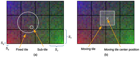
Figure 9.
Positioning area divided into 12 fixed tiles and a moving tile. Fingerprints color-coded for different positions. The side length of the sub-tile is ; the side length of the tile is . (a) Details of a fixed tile. (b) Details of a moving tile.
Dividing the whole positioning area into perfect area fractions can ideally be achieved by sampling contiguous parts of the whole area; moving the 2D sensor array to the next position, without overlapping; and repeating this process until the whole area is covered. For example, in Figure 9, the whole positioning area can be sampled by placing the 2D sensor array within the 12 area fractions depicted in the figure. In practice, this is difficult to achieve; however, by sampling at the positions where the samples of the sensors overlap, an equivalent result can be achieved by post-processing the sampled fingerprints. Assuming uniform statistics for the fingerprints, the fingerprints at overlapping subdivisions can be discarded.
The discretized area fractions mentioned above are called tiles in the context of this work. So, in Figure 9, the positioning areas are actually divided into 12 (fixed) tiles. We assign these the name tiles due to the resemblance of dividing the whole positioning area into area fractions with the grid pattern outlined by square tiles. Thus, the process of dividing the positioning area into tiles is referred to as tiling. It is recalled that there is a direct relationship between a tile and the 2D sensor array. The 2D sensor array is actually the one sampling the whole positioning area into area fractions equal to its size and generating the tiles. Then, each sensor in the 2D sensor array is analogous to a subdivision in the tile, which we call a sub-tile. It is assumed that the sub-tile is the smallest granularity for discretizing the positioning area and sample positions. Since a vector of fingerprints is collected at each sensor in the 2D sensor array, there is a vector of fingerprints associated with each sub-tile.
An example of tiles and sub-tiles is depicted in Figure 9a. The tiles depicted in the figure have a square shape; however, these could have any other shape if desired. In the context of this work, we will work only with square tiles. We assume a uniform size for the sub-tiles within the tiles (or sensors within the 2D sensor array). The side length of a sub-tile is indicated by . The size of a tile, and thus the 2D sensor array, is measured by the number of sub-tiles per side of the tile (that is, the number of sensors per side of the 2D sensor array), , for a given side length of a sub-tile. The side length of a tile is indicated by , with . For a square tile, there are a total of sub-tiles in a tile, with . The parameters and variables related to the tiles and sub-tiles (and correspondingly associated with the 2D sensor array) are summarized in Table 5. Finally, we assume that the whole positioning area is covered by an integer total number of tiles, . That is, it is assumed that the tiles cannot be divided into smaller fractions.
Table 5.
Parameters and variables for tiles (2D sensor array).
Tiles covering the whole positioning area uniformly, with a contiguous arrangement as a grid and non-overlapping, as depicted in Figure 9a, are referred to as fixed tiles. Fixed tiles are tiles that have associated fingerprints used in the training phase. Thus, the tiling of the positioning area with fixed tiles, in a contiguous arrangement as a grid, is used only in the training phase. Such a grid-like arrangement is an aid in developing the pattern-matching methods.
In the testing phase, when one intends to find a position, the grid-like arrangement of fixed tiles is unknown. In the testing phase, for a random position within the whole positioning area, not constrained to the positions of the fixed tiles from the tiling process, the 2D sensor array will describe a tile that, in general, it is not aligned with the fixed tiles of the grid-like arrangement. A tile described by the 2D sensor array at a random position within the positioning area is referred to as a moving tile. In other words, moving tiles are the products of the samples generated using the 2D sensor array at random positions. In the context of this work, moving tiles will be generated at random positions to benchmark different pattern-matching methods in the testing phase. An example of a moving tile is shown in Figure 9b. It is assumed that a moving tile always keeps the same orientation as the fixed tiles in the grid-like arrangement described by the fixed tiles, or in other words, it is not rotated. Finally, to estimate a position during the testing phase, an algorithm implementing a pattern-matching method will use as its input the fingerprints collected from the 2D sensor array, acting as a moving tile, and compute the estimated position of the 2D sensor array. The pattern-matching method is previously trained in the training phase with information from the fixed tiles.
It is noted that in the scope of our work, in the training phase, we choose to discretize the positioning area with a contiguous arrangement of non-overlapping fixed tiles as a grid. From one perspective, it could be thought that such discretization does not offer sufficient sampling of the positioning area in the sense that the training is carried out at the discrete positions delimited by the fixed tiles, whereas the testing is carried out at random positions that may occur in between the discretized positions used for the training. However, we recall that our primary goal is to learn whether the use of spatial side information produces a gain over the case of not using such side information. It is not relevant to our scope whether the use of side information with an arrangement of tiles with or without overlapping produces an optimal result. Within our scope, it is enough that we can observe that there is some gain with the proposed approach using non-overlapping tiles. From another perspective, the discretization with the tiles helps us retain consistency for comparing the different pattern-matching methods considered, in the sense that comparisons of the outputs are performed for the same inputs. One of the pattern-matching methods is based on classification, in which we need to discretize the positioning area into distinctive classes. Therefore, we base our study on the use of discretized fractions of the positioning area in the form of non-overlapping tiles. A comparison against cases with overlapping tiles, or any other arrangement using side information, is deferred to future work.
4.3. Positioning Process
The process for positioning using spatial side information proposed in our work is summarized as follows.
- The training phase: In a given positioning area, we create an ideal grid-like arrangement of fixed tiles. Each fixed tile corresponds in its size to the size of the 2D sensor array and in the number and size of the sub-tiles to each sensor in the 2D sensor array. The 2D sensor array is aligned with a fixed tile to sample fingerprints with adjacent side information. Fingerprint samples are collected from each sensor in the 2D sensors array and assigned to a vector of fingerprints. In turn, the vector of fingerprints is associated with a sub-tile. The elements in the vector of fingerprints are the fingerprints obtained from each fingerprint source. For a number of fingerprint sources, the vector has elements. The fingerprints from the whole 2D sensor array are associated with a tile and assigned to a tensor of fingerprints, with the dimensions .Fingerprint samples from fixed tiles, along with the reference ground truth positions, are used to train a regression-based FFNN model with a given pattern-matching method. Alternatively, fingerprint samples from fixed tiles, along with the tile-class labels, are used to train a classification-based CNN model with a given pattern-matching method. The training of all of the models is based on supervised learning.
- The testing phase: A positioning device implementing a 2D sensor array is placed at some random position within the positioning area. The position of the 2D sensor array determines what is thought of as a moving tile. The 2D sensor array samples fingerprints with adjacent side information. As in the case of fixed tiles, fingerprint samples are collected from each sensor in the 2D sensor array, which are associated with a sub-tile and assigned to a vector of fingerprints, with elements obtained from each fingerprint source. The fingerprints from the whole 2D sensor array are associated with a moving tile and assigned to a tensor of fingerprints, with the dimensions . Finally, the position estimate is calculated using all of the pattern-matching methods constructed in the training phase, using as the input the tensor of fingerprints associated with the moving tile.
- Comparison of the results: This consists of comparing the performance among all of the proposed pattern-matching methods considered in terms of the error distance, , given by Equation (1).
4.4. Pattern-Matching Methods
The pattern-matching methods selected in our study comprise first the traditional fingerprinting method without side information and then three pattern-matching methods exploiting spatial side information. We assign a mnemonic name to each one of the four pattern-matching methods selected, namely 1-SingFingIn-PosOut, 2SingFingInAggPosOut, 3-MultFingIn-PosOut, and 4-MultFingIn-ClassOut. These are summarized in Table 6, shown in Figure 10, and explained below.
Table 6.
Pattern-matching methods.
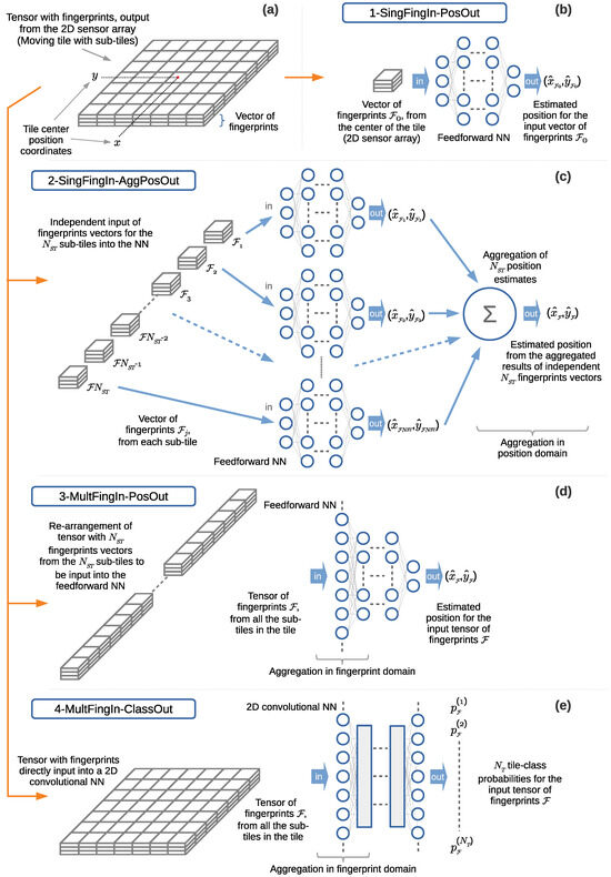
Figure 10.
Fingerprinting pattern-matching methods. (a) 2D sensor array. (b) Method 1-SingFingIn-PosOut. (c) Method 2-SingFingIn-AggPosOut. (d) Method 3-MultFingIn-PosOut. (e) Method 4-MultFingIn-ClassOut.
The mnemonic names assigned to the pattern-matching methods listed in Table 6 compress the information described next. The mnemonic 1-SingFingIn-PosOut stands for patternmatching method number one, taking a single vector of fingerprints as the input from a single sub-tile and producing a position as the output. The mnemonic 2-SingFingIn-AggPosOut stands for pattern-matching method number two, taking a single vector of fingerprints as the input for each one of sub-tiles independently and producing a position as the output. In this last method, the output results from aggregating independent position estimates. The mnemonic 3-MultFingIn-PosOut stands for pattern-matching method number three, taking multiple fingerprints as the input and producing a position as the output. The mnemonic 4-MultFingIn-ClassOut stands for pattern-matching method number four, taking multiple fingerprints as the input and producing a tile-class probability as the output.
The positioning data aggregation domains listed in Table 6 and their relationships to the patternmatching methods are consistent with those introduced in Section 2.4 and listed in Table 2.
All of the pattern-matching methods take as their input the fingerprints collected through the 2D sensor array, shown in Figure 10a. The 2D sensor array returns a tensor with a set of fingerprints . The tensor can be interpreted as a 2D arrangement of a total of fingerprint vectors, where each vector contains elements. Each element of a vector is a fingerprint from one of the fingerprint sources.
4.4.1. Pattern-Matching Method 1-SingFingIn-PosOut
The pattern-matching method 1-SingFingIn-PosOut consists of the traditional fingerprinting method based on associating a vector of fingerprints with a position, without spatial side information on the fingerprints. It maps a vector of fingerprints collected at a single, pointwise, position to the final position estimate. This method is depicted in Figure 10b.
The method consists of calculating a position estimate using only a single sub-tile—for example, the central sub-tile. In the training phase, an FFNN with inputs, with one for each fingerprint, is trained as a regression model. The input to the NN is a vector with elements that form a set of fingerprints. These fingerprints are the ones measured in a selected reference sub-tile of a fixed tile. The training aims to map the input fingerprints to a reference ground truth position associated with the tile or to a reference position in the selected sub-tile. The final goal is to tune the parameters in the NN to produce as the output a position estimate for the selected reference position for a given set of input fingerprints.
In the testing phase, the FFNN takes as the input a vector of fingerprints from a sub-tile in a moving tile. The selected sub-tile is consistent with that used in the training phase. The FFNN produces as its output a position estimate consistent with the reference position used in the training phase, with the coordinates and .
Regarding the selection of a reference sub-tile, we suggested above to use the central sub-tile. In cases with an even number of sub-tiles per side, the central sub-tile can be defined as one of the four closest to the center of the tile. Alternatively, the center of the tile, or any other part of the tile, can be used as the training target position. Regardless of the point of the tile selected as the target training position, it is important to use the same point in the tile for the reference ground truth position when calculating the positioning error to avoid introducing a systematic error.
4.4.2. Pattern-Matching Method 2-SingFingIn-AggPosOut
The pattern-matching method 2-SingFingIn-AggPosOut uses spatial side information on the fingerprints. It produces the position estimate by aggregating the position estimates for each sub-tile in a tile in the position domain. This method is depicted in Figure 10c.
The method consists of calculating a position estimate from a single sub-tile independently from the others for all of the sub-tiles in a tile. This method can be thought of as an extension of the pointwise case, in which the method 1-SingFingIn-PosOut is applied to each sub-tile instead of to a single sub-tile. Then, there is a position estimate for each sub-tile. The position estimates for all of the sub-tiles are aggregated in the position domain to produce a final position estimate for the tile. This is similar to sampling the pointwise positions in a small area sequentially in the time domain by means of a single sensor or receiver, with posterior aggregation of the position estimates. The difference here is that we take many samples at once using the 2D sensor array.
In the training phase, an FFNN with inputs, with one for each fingerprint, is trained as a regression model. The input to the NN is a vector with elements that form a set of fingerprints. Here, j is a sub-tile from a set of sub-tiles from a fixed tile, with . The training aims to map the input fingerprints associated with the sub-tile j to the reference position of sub-tile j. We consider here a case in which there is a single and common NN trained against the fingerprints for sub-tiles. The final goal is to tune the parameters in the NN to produce as the output a position estimate for the reference position of the sub-tile associated with a given set of input fingerprints.
In the testing phase, the FFNN takes as its input one vector with elements that form a set of fingerprints from one sub-tile j in a moving tile, with . The FFNN produces as its output a position estimate for the sub-tile j, with the coordinates and . Here, each one of the vectors of fingerprints is associated with each one of sub-tiles. This process is repeated for each one of the sub-tiles in the moving tile. Finally, the position estimates for each sub-tile are aggregated to produce a final position estimate for the tile, with the position coordinates and . In the implementation of this pattern-matching method, the position estimates for each sub-tile are aggregated by the mean value:
and
We note that the mean value in Equations (2) and (3) is a simplification of an averaging operation in which it is assumed that the reference position of a tile is the center of the tile, and the reference position of a sub-tile is the center of the sub-tile. With this assumption, an offset, positive or negative, from the center of the tile is incorporated into the estimated position of each sub-tile, in the sense that this offset is present in the training phase. Then, by considering as the reference position the center of the tile, the positive and negative offsets of the sub-tiles from the center of the tile are canceled out in the sum, and therefore, it is not necessary to include these in the equations.
4.4.3. Pattern-Matching Method 3-MultFingIn-PosOut
The pattern-matching method 3-MultFingIn-PosOut uses spatial side information on the fingerprints. It produces a position estimate by aggregating the fingerprints from all of the sub-tiles in the fingerprint domain. The aggregation of the fingerprints is carried out using an FFNN. This method is depicted in Figure 10d.
The method consists of calculating a position estimate from all of the sub-tiles. In the training phase, an FFNN with inputs takes all of the fingerprints from all of the sub-tiles of a fixed tile at once as the input. The input to the NN is a tensor of fingerprints , constructed with vectors of fingerprints each one. The NN is trained as a regression model to map the input tensor of fingerprints to a reference ground truth position associated with the tile.
In the testing phase, the FFNN takes as its input all of the fingerprints from a moving tile and produces as its output a position estimate with the coordinates and , consistent with the reference position used in the training phase.
4.4.4. Pattern-Matching Method 4-MultFingIn-ClassOut
The pattern-matching method 4-MultFingIn-ClassOut uses spatial side information on the fingerprints. It produces a classification of the tiles as tile-classes based on fixed tiles by aggregating the fingerprints from all of the sub-tiles in the fingerprint domain. The aggregation of the fingerprints is carried out using a 2D CNN. The position estimate is calculated by relying on the classification of the fixed tiles and a mapping between the tile-class labels and the positions of the corresponding fixed tiles. This method is depicted in Figure 10e.
The use of a CNN is promising for the problem at hand. The CNN presents an architecture implementing the convolution operation which may be suitable for exploiting the side information and offering an optimal representational capacity. The architecture of the CNN may require the use of a large number of parameters to generalize the model. In comparison, using an equivalent number of parameters in an FFNN would result in overfitting and thus the model not being generalized. From this perspective, it is expected that for the same number of parameters, a CNN can provide a higher performance than an FFNN in terms of minimizing the error distance. As mentioned in Section 5.7.1, we observed that increasing the width or depth of the layers in the FFNN, after certain point, does not produce an improvement in performance.
The approach in this method is analogous to that used in image classification problems and pattern recognition in images, which apply a convolution operation using 2D CNNs. In traditional image processing, the images usually have one channel (monochrome images) or three channels (RGB colors). In contrast, we will use a 2D CNN as it is used in image classification problems; however, the images will be in the form of a tensor of fingerprints, as detailed next. The tensor input to the CNN has two dimensions for the 2D spatial position coordinates associated with the fingerprints measured by the 2D sensor array and a third dimension for the channels. The channels in this case represent each one of the fingerprints from fingerprint sources. The training phase is carried out with fixed tiles, associated with definite tile-classes. The testing phase for the actual positioning is carried out with moving tiles. The objective is to estimate the positions of the moving tiles. We recall that there is a direct relationship between a tile and the 2D sensor array. Here, we expect from the CNN an output result showing a higher classification probability for the tile-classes (associated with fixed tiles) that are closer to the target input moving tile. Then, this method will combine the known positions of the fixed tiles and the hit probability for these to estimate the position of the target moving tile (2D sensor array).
Figure 11 shows an example of the tile-class labels assigned to fixed tiles (the numbers inside circles) and the border of a superimposed random moving tile. For a given input of fingerprints, here that corresponding to a moving tile, the 2D CNN returns as its output the tile-class probabilities associated with each fixed tile. The figure shows as an example an ideal outcome where the 2D CNN returns as its output tile-class probabilities that are proportional to the areas of the fixed tiles covered by the overlapping part of the moving tile (percentages shown at the bottom of each fixed tile).
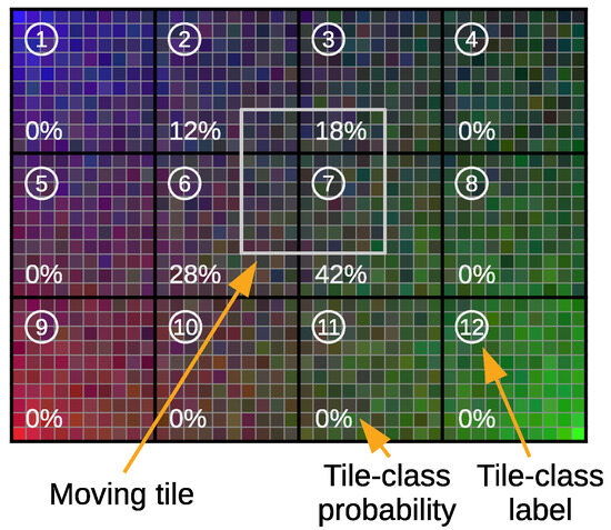
Figure 11.
Example of tile-class labels assigned to the fixed tiles (numbers inside circles) and the border of a superimposed random moving tile. For a given input of fingerprints, here that corresponding to the moving tile, the 2D CNN returns as its output tile-class probabilities (associated with each fixed tile). Here, we exemplify an ideal outcome where the tile-class probabilities are proportional to the areas of the fixed tiles covered by the overlapping part of the moving tile (percentages shown at the bottom of each fixed tile).
A moving tile can overlap with 1 to 4 fixed tiles. However, moving tiles most likely will be shifted from the fixed tiles and thus will most likely overlap with 4 fixed tiles. Ideally, the RSS fingerprints in the overlapping sub-tiles of a moving tile and a fixed tile will match. In practice, these will differ due to the presence of noise and other effects. Noise and other effects contribute a random component to the fingerprints (for example, shadow fading in the case of radio signals). However, the fingerprints from the fixed and moving tiles in the overlapping parts will bear resemblance to some extent, such that these can be recognized by the 2D CNN as a translation of part of a fixed tile with a certain tile-class probability.
A 2D CNN takes as its input a tile in the form of a tensor of fingerprints , interpreted as a 2D image with channels, produced by the 2D sensor array. The input tensor has a size given by the size of the 2D sensor array and the number of channels (equivalent to the number of fingerprint sources, ). In the training phase, the CNN is trained with fixed tiles as a classification model to map the fingerprints to a fixed tile tile-class. The CNN outputs a tile-class likelihood probability vector, , of size , indicating the likelihood of matching each tile-class for the tiles available in the positioning area in a target scenario. The tile-class likelihood probability vector is the output of the NN from a normalized dense layer with a softmax activation function.
In the testing phase, the CNN takes as its input the tensor of fingerprints of the size from a moving tile and produces as its output the tile-class likelihood probability vector . A known mapping between the tile-classes and the center positions of the respective fixed tiles is used to calculate the estimated position coordinates, and , of the moving tile (2D sensor array).
The final position coordinate estimate, and , for a given input tensor with fingerprints is calculated by aggregating the tile-class probabilities assigned as weights to the position coordinates of the corresponding fixed tiles:
where is the set of fixed tiles, with cardinality and elements , and are the coordinates of the center of the tile j, and is the th element of the tile-class likelihood probability vector , associated with the tile j, where
It is assumed that there is a suitable data structure, e.g., a look-up table, with the mapping between the tile-class j and its center coordinates and .
Other ways to exploit the tile-class probabilities output by the softmax layer could be devised. However, our goal is to investigate the possible gains with the proposed approach, so other ways to exploit the tile-class probabilities are left for future work.
- ○
- Translation Invariance PropertyIt is unclear to us whether the so-called translation invariance property of CNNs is present and contributing to boosting the recognition of parts of a moving tile, which are translated parts of the overlapped fixed tiles. This translation invariance property is also discussed in terms of shift invariance [209]. It is under debate whether the architecture of CNNs alone, the introduction of multiple convolutional layers, the introduction of pooling layers, data augmentation, or a combination of the former contributes to the translation invariance property. In [210], translation invariance is discussed in terms of a local translation, enabled by pooling functions, for small translations in the input. In [211], it is concluded that for the processing of images, the invariance increases with the depth of the CNN. In [212], it is concluded that CNNs alone are not translation-invariant but that the main contribution to the invariance is the training with the help of data augmentation. It is argued that CNNs are not shift-invariant due to the presence of downsampling, introduced by layers like strided max-pooling [213,214].We implemented a CNN without pooling and without data augmentation in the translation domain (meaning that we augmented data by introducing a random shadow fading component into each sub-tile, but the base path loss component remained constant for the position of each sub-tile, and thus, there was no augmentation through translation in the fixed tiles used for training). Thus, according to the claim of some works in line with those cited above, our CNN does not benefit from the translation invariance property. Yet as a matter of fact, the CNN implemented manages to find with a high probability fixed tiles that resemble moving tiles. Given that the tile-classes from the fixed tiles present a variation in a pattern that can be considered almost continuous, it is unclear to us whether the good performance observed is because the fixed tiles are identified by moving tiles with a close resemblance and/or because the good performance is enabled by the translation invariance. A reasoning in line with the possible contribution of the translation invariance is based on the assumption that the pattern described by a fixed tile, notwithstanding the noise component introduced by the shadow fading, can be found in the parts of a moving tile regardless of the position of the pattern in the tile. Parts of these patterns can be at different positions in the moving tile compared with in a fixed tile. Then, if translation invariance exists, we would expect to observe that the parts of a moving tile can be identified with a higher probability in fixed tiles around the moving tile.
- ○
- Tile-class Probabilities and Data Aggregation DomainsIt is open to discussion whether the processing of the tile-class probabilities, along with the known tile center positions, is regarded as positioning data aggregation in the position domain. The input fingerprints are aggregated in the fingerprint domain by the CNN; therefore, there is not a one-to-one mapping from an individual fingerprint to each tile-class probability. Therefore, we do not treat this step as an aggregation in the position domain, in as much as we do not treat as aggregation in the position domain the last layers in the pattern-matching method 3-MultFingIn-PosOut, which ultimately aggregates the NN data to calculate the final output position estimate.
5. Feasibility Study Through System Simulations
In this section, we carry out a feasibility study using simulations to learn whether the use of spatial side information on the fingerprints can lead to a justifiable gain in terms of minimizing the positioning error. This study is performed using simulations based on Monte Carlo methods with a system simulator, testing the performance of each pattern-matching method with synthetic fingerprints and moving tiles at random positions.
Monte Carlo methods are suitable for studying the behavior of complex systems. In the field of telecommunications, Monte Carlo methods are a common way to study the performance of a communications system at the system level. The system-level approach abstracts the actual information transmitted at the bit level over the communication links with a representation at the signal level. In the context of this work, we work with RSS-based fingerprints, which are generated in the same way as they are in system-level simulators for communications systems.
Our system is composed of the 2D sensor array used to collect fingerprint samples with adjacent side information (Section 4.1); a scenario constituting four base stations and the area intended for positioning (Section 5.1) discretized into tiles (Section 4.2) of a given size (Section 5.9) in the training phase; and the fingerprinting-based positioning method, based on the mapping of the fingerprints to positions using a pattern-matching method (Figure 5, Section 2.2) by implementing an NN.
Four pattern-matching methods are implemented, as described in Section 4.4 and depicted in Figure 10.
Data collection from field measurements is very costly, in particular for feeding machinelearningbased models as training data. Thus, in this study, we rely on synthetically generated fingerprints in the form of the RSS. Synthetic data generation for positioning is not uncommon in the literature. In [215], synthetic data are generated to augment a small set of measured data for localization purposes, and a simulator is used for the evaluation of the proposed solution. In [216], the generation of fingerprints using radio propagation models is presented as virtual fingerprinting. In [217], an algorithm is validated and tested with the aid of simulations, and synthetic data are generated to complement measured positioning data in the training phase for an NN-based model. Other examples of works implementing synthetic fingerprints are [143,151,189]. From another perspective, regardless of the number of channels used to create the fingerprint images for pattern-matching method 4-MultFingIn-ClassOut, the creation of fingerprint images can be considered a subcategory of the more general fields of synthetic image generation and image synthesis [218,219,220].
The implemented system simulator comprises the following:
- The creation of a scenario with transmitting base stations in downlink and the area intended for positioning;
- Tiling of the area intended for positioning (creation of the positioning area);
- The creation of datasets of synthetic fingerprints for fixed and moving tiles (as arrangements that are equivalent to samples of the 2D sensor array) with a radio channel model, published by a standardization body, for a frequency of GHz;
- Training of the NN model for a selected patternmatching method in the training phase;
- Estimation of the positions of moving tiles in the testing phase;
- Storage of the best-performing result.
Simulations are carried out for the four pattern-matching methods introduced in Section 4.4 for processing the fingerprints. The first pattern-matching method is based on the traditional approach to pointwise samples, without side information. The other three pattern-matching methods use spatial side information. All of the pattern-matching methods are benchmarked against each other, primarily to learn whether the use of spatial side information brings some gain and secondarily to learn how the different pattern-matching methods that process the side information perform against each other. We investigate the performance of the four pattern-matching methods from the results of the simulations in the next section.
The next subsections explain the different components of the system simulator and provide details of the simulation process, simulation execution, the NN structure for each pattern-matching method, and other relevant considerations.
5.1. Scenario for Simulations, Area Intended for Positioning, and Positioning Area
A scenario with an LOS radio propagation channel model is selected because it is a challenging scenario for fingerprinting-based positioning. Such a scenario is suitable for benchmarking positioning with spatial side information. Fingerprinting-based positioning exploiting RSS fingerprints benefits from abrupt changes in the RSS. For example, in [221], the abrupt change in the radio signal’s strength through a wall is exploited to distinguish between different rooms. In [222], a physical arrangement consisting of an air-gap between attenuating surfaces is used to create a distinctive radiation pattern for the radio signal, which results in an abrupt change in the RSS. This abrupt change is tested for fingerprinting-based positioning against the signal strength that would be produced by an omnidirectional antenna without any object attenuating the radio signal. It is concluded that with such an abrupt change in the RSS, the positioning error is reduced. In [82], a reconfigurable intelligent surface is used to produce distinctive differences in the RSS in adjacent locations. Contrary to these research works, in our study, we intend to avoid such abrupt changes in the RSS so that the observed performance results are solely based on the gains produced by the spatial side information attained through the 2D sensor array. Therefore, we will assume an omnidirectional radiation pattern for the antennas of the transmitters and an LOS radio propagation channel model.
To evaluate the proposed pattern-matching methods, the following scenario is proposed for the simulations. The scenario consists of an open area available for positioning with a maximum size of 13 m by 5 m. This open area is free of objects to allow the LOS propagation of the radio signal. Hereafter, this area is referred to as the area intended for positioning. The area intended for positioning spans from position 1 m to 14 m in the x coordinates and from position 1 m to 6 m in the y coordinates in the scenario. Positioning takes place within an area referred to as the positioning area and which is inscribed in the area intended for positioning. So, in other words, the positioning area is a rectangle inscribed within the area intended for positioning, where the former can be smaller or equal to the latter.
The positioning area is the actual area in which we study the different pattern-matching methods using simulations. It is noted that the positioning area can vary in size as a function of the selected tile sizes; however, it is constrained to a maximum size of m2 (the area intended for positioning in the scenario). Actually, we set a constraint on not allowing the use of fractions of a tile to cover the area intended for positioning. So, for some tile sizes, the positioning area will be equal to the area intended for positioning, and for other tile sizes, the positioning area will be slightly smaller than the area intended for positioning. The use of different tile sizes, border conditions, and the resulting positioning areas is discussed in Section 5.3. In the example that follows (Figure 12), the example in Section 5.2.4, as well as in the explanation of one of the results obtained (first example in Section 6.8.3), the area intended for positioning and the positioning area coincide. In contrast, in the second example presented in Section 6.8.3, the area intended for positioning and the positioning area differ. The difference between these areas can be observed in the figure of the second example in the cited section.
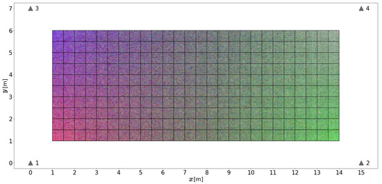
Figure 12.
Scenario layout depicting the positions of four base stations (triangles) and the area intended for positioning. As an example, the selected size of the tiles results in a positioning area equivalent in size to the area intended for positioning. The positioning area is fully covered by fixed tiles (colored region) and shows one snapshot of the radio channel state. Each sub-tile has a vector of fingerprint elements from the four base stations associated with it, which is color-coded with the RGB and opacity channels. In the example shown, all of the tiles cover the area intended for positioning with , and mm.
The scenario is shown in Figure 12. In the figure, as an example, the area intended for positioning (13 m by 5 m) is fully covered by the positioning area with the selection of tiles with side lengths of 500 mm. In this case, the dimensions of the area intended for positioning, 13,000 mm × 5000 mm, are multiples of the dimensions of the tile, and thus an exact number of tiles fits into the area intended for positioning. The positioning area is colored with red, green, and blue. The base stations are depicted in the figure with four triangles numbered from one to four and are located in this scenario in the positions listed in Table 7.
Table 7.
Base station positions in the scenario.
Figure 12 depicts an example in which the whole positioning area is covered by fixed tiles of the size 500 mm by 500 mm, with , and mm, to exemplify the tiling of the area intended for positioning (the creation of the actual positioning area). As described in Section 4.2, each sub-tile has a vector of fingerprints associated with it. Here, the elements in the vector of fingerprints are the RSS values received in downlink from the four base stations. Aligned with this, in Figure 12, each sub-tile is color-coded with the RGB channel colors and the opacity from the alpha-channel to represent the fingerprints from each one of the four base stations. The signal strength from base stations 1, 2, and 3 is coded in the colors red, green, and blue, respectively. The signal strength from base station 4 is coded as the opacity from the alpha-channel. The color strength or opacity decreases with the distance from each base station, analogous to the attenuation in the RSS of the radio signal. In addition, the RSS contains a random component that models the shadow fading. In the figure, this random component is depicted by the lack of gradual uniformity in the continuity of the colors between adjacent sub-tiles. The color coding is used to create a visual aid showing that the fingerprints vary with the position and the shadow fading. This example shows one snapshot in time of the time-varying radio channel state. Hereafter, we refer to this snapshot in time as radio channel realization.
5.2. Generation of Datasets of Fingerprints
Four datasets of fingerprint data are synthetically generated: first, a dataset of fixed tiles for training the NN, labeled as Fixed Tiles for Training (FTT); second, a dataset of fixed tiles for validation of the trained NN model, labeled as Fixed Tiles for Validation (FTV); third, a dataset of moving tiles for validation, labeled as Moving Tiles for Validation (MTV); and fourth, a dataset of moving tiles for testing, labeled as Moving Tiles for Testing (MTT). The datasets are labeled as indicated in Table 8. The first two datasets associate fingerprints with fixed tiles, and the last two datasets associate fingerprints with moving tiles.
Table 8.
Acronyms for datasets.
5.2.1. Validation Datasets
Two validation datasets are used. The FTV dataset is used to select the set of training weights that produce the minimum error among the training epochs. The MTV dataset is used to select the set of training weights that produce the minimum error among different initial random weights.
The rationale behind the use of two validation sets is as follows. The training phase is carried out with a dataset of fixed tiles (FTT); however, the trained NN model is expected to generalize for a testing dataset of moving tiles (MTT). Then, for the selection of the best training weights among epochs and aiming to reduce the generalization error, we rely on a validation dataset of fixed tiles (FTV), which is consistent with the dataset type used for the training. However, as the target testing dataset consists of moving tiles (MTT), we use a second validation dataset, this time with moving tiles (MTV). The use of the MTV dataset aims to reduce the generalization error using moving tiles by selecting the weights that produce the minimum error metric in the performance of the model among different initial random weights. Since we are trying to optimize a non-convex problem, the training of the model is repeated a number of times with different initial random weights in an attempt to obtain the most favorable solution (as will be explained in step ⑤ of the execution flow of the model training presented in Section 5.6.3).
5.2.2. Generation of the Center Position Coordinates for Fixed Tiles
The number and positions of fixed tiles are a function of the number of sub-tiles per side of the tile, , and the side length of the sub-tile, . Prior to the generation of the datasets, the center position coordinates for the fixed tiles are determined. Pseudocode 1 shows the function , which is in charge of calculating the center position coordinates for the fixed tiles. It is noted that this function does not generate the actual tiles, but it just generates the coordinates of an imaginary grid that will hold the fixed tiles. The actual fixed tiles will be generated using another function. One function call is made to (as will be explained in step  of the main execution flow of the simulator presented in Section 5.6.1). The function returns as the output a data structure with an arrangement of the fixed tiles’ centers, for example, in the form of a vector, array, or list, for each coordinate, namely and . These data structures are used next to generate datasets of fixed tiles in the function and to define the area allowed for generating the datasets of moving tiles in the function . This function also calculates and returns as output the total number of tiles required to cover the whole positioning area, .
of the main execution flow of the simulator presented in Section 5.6.1). The function returns as the output a data structure with an arrangement of the fixed tiles’ centers, for example, in the form of a vector, array, or list, for each coordinate, namely and . These data structures are used next to generate datasets of fixed tiles in the function and to define the area allowed for generating the datasets of moving tiles in the function . This function also calculates and returns as output the total number of tiles required to cover the whole positioning area, .
| Pseudocode 1 Function for calculating the center positions for fixed tiles - FTileCenters() |
|
It is noted that, in order to present a simple and compact structure for the simulator, the scenario dimensions for the area intended for positioning are hard-coded into the function. So, for a given input of parameters and , the function defines the center positions of the fixed tiles and in the end returns as the output the final positioning area.
5.2.3. Generation of Fixed Tiles
Pseudocode 2 shows the function , which is in charge of generating the datasets with fixed tiles, FTT and FTV. This function takes as its input the center position coordinates of the fixed tiles and generates fixed tiles at the specified positions. The function also takes as input the number of fixed tile batches , which determines how many batches of tiles are generated. Each batch covers the entire positioning area in the scenario. Thus, there are instances of tiles at each tile position, each with a different set of radio channel realizations (vector of fingerprints) in each sub-tile. The radio channel realizations result from the path losses from the base stations and the randomness introduced by the shadow fading in the radio channel model (Section 5.4). Each channel realization most likely determines a different set of fingerprints at each tile position. In our simulations, we use the same number of batches, , for the FTT and FTV datasets. The function makes calls to the function , which is the one in charge of generating the actual tile (one per call), with the corresponding fingerprints at the given tile coordinates. The function also takes and as input with the purpose of passing these as input to the function .
| Pseudocode 2 Function for generating fixed tiles - FFixedTiles() |
|
A data structure in the form of a vector, array, or list is returned as output, in which each element is a tensor, or another suitable data structure, associated with a tile for storing the fingerprints. This tensor or data structure contains as elements the vectors of fingerprints for each sub-tile in the tile. The function also returns as output a data structure in the form of a vector, array, or list, in which each element contains a data structure associated with a tile and consistent in indexing order with a tile in . This data structure contains the reference center position coordinates for each generated sub-tile in the tile.
For simplicity, the pseudocode for the function does not show that each fixed tile needs to have a tile-class label associated with it. The tile-class label is any distinctive indicator, which ultimately is vectorized using one-hot encoding. It is assumed that this or another function creates such a label and that a suitable data structure, for example, in the form of a look-up table, is created to map each tile-class label to the center position of the corresponding fixed tile. The tile-class label, and the data structure mapping the tile-class to the center position of the fixed tile, are used by pattern-matching method 4-MultFingIn-ClassOut, which is a classification-based method.
Two function calls to are performed, one to generate the FTT dataset and one to generate the FTV dataset (as will be explained in steps  and
and  of the main execution flow of the simulator presented in Section 5.6.1). Figure 12 depicts an example of the output produced by this function for one batch, in which the area intended for positioning is fully covered by fixed tiles. The figure also depicts an example of one radio channel realization. Each sub-tile has a vector of fingerprint elements from the four base stations associated with it. In the figure, each sub-tile is color-coded with the RGB and opacity channels to represent the fingerprints from each one of the four base stations. In this example, , and mm.
and of the main execution flow of the simulator presented in Section 5.6.1). Figure 12 depicts an example of the output produced by this function for one batch, in which the area intended for positioning is fully covered by fixed tiles. The figure also depicts an example of one radio channel realization. Each sub-tile has a vector of fingerprint elements from the four base stations associated with it. In the figure, each sub-tile is color-coded with the RGB and opacity channels to represent the fingerprints from each one of the four base stations. In this example, , and mm.5.2.4. Generation of Moving Tiles
Pseudocode 3 shows the function , in charge of generating the datasets with moving tiles, MTV and MTT. This function takes as input the center position coordinates of the fixed tiles to determine the area in which the moving tiles can be generated (details on the allowed positioning area are provided below in Section 5.3). This function also takes as input , which determines how many moving tiles are generated. The position of the moving tiles is determined randomly, with the outcome of pseudo-random numbers generated from a uniform distribution in the interval , , scaled and shifted to the dimensions of the positioning area. Each moving tile has a set of radio channel realizations (vector of fingerprints) in each sub-tile, resulting from the path losses from the base stations and the randomness introduced by the shadow fading in the radio channel model (Section 5.4). Thus, each channel realization most likely determines a different set of fingerprints at each tile position. In the simulations, we use . The function makes calls to the function , which is the one in charge of generating the actual tile (one per call), with the corresponding fingerprints, at the given tile coordinates. This function also takes as input and , with the purpose of passing these as input to the function .
| Pseudocode 3 Function for generating moving tiles - FMovingTiles() |
|
A data structure in the form of a vector, array, or list is returned as the output, in which each element is a tensor, or another suitable data structure, associated with a tile for storing the fingerprints. This tensor or data structure contains as its elements the vectors of fingerprints for each sub-tile in the tile. This function also returns as output a data structure in the form of a vector, array, or list in which each element contains a data structure associated with a tile and consistent in indexing order with a tile in . This data structure contains the reference center position coordinates for each generated sub-tile in the tile.
Two function calls to are performed, one to generate the MTV dataset and one to generate the MTT dataset (as will be explained in steps  and
and  of the main execution flow of the simulator presented in Section 5.6.1). Figure 13 depicts an example of the output produced by this function for 40 moving tiles (colored tiles). In the figure, the positioning area for this example is the grid that spans from position 1 m to 14 m along the x coordinates and from position 1 m to 6 m along the y coordinates. This positioning area is analogous to the one depicted in Figure 12 for fixed tiles. The grid is provided as a reference to observe the relative position of the moving tiles to the actual position of the fixed tiles. Each sub-tile of the moving tiles has a vector of fingerprint elements from the four base stations associated with it. In the figure, each sub-tile is color-coded with the RGB and opacity channels to represent the fingerprints from each one of the four base stations. In this example, , and mm.
and of the main execution flow of the simulator presented in Section 5.6.1). Figure 13 depicts an example of the output produced by this function for 40 moving tiles (colored tiles). In the figure, the positioning area for this example is the grid that spans from position 1 m to 14 m along the x coordinates and from position 1 m to 6 m along the y coordinates. This positioning area is analogous to the one depicted in Figure 12 for fixed tiles. The grid is provided as a reference to observe the relative position of the moving tiles to the actual position of the fixed tiles. Each sub-tile of the moving tiles has a vector of fingerprint elements from the four base stations associated with it. In the figure, each sub-tile is color-coded with the RGB and opacity channels to represent the fingerprints from each one of the four base stations. In this example, , and mm.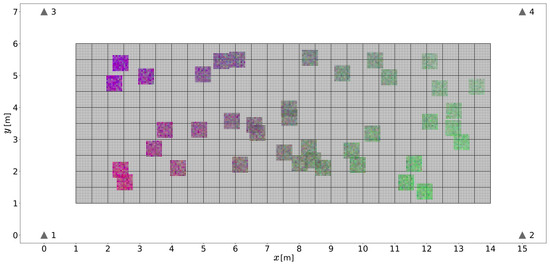
Figure 13.
Example of 40 moving tiles (colored tiles) with and mm generated by samples obtained from a uniform distribution in the function . The grid covering the positioning area is provided as a reference to observe the relative position of the moving tiles to the actual position of the fixed tiles.
5.2.5. Generation of Individual Tiles
The functions and create fixed and moving tiles, respectively. The difference between these functions is the following. The function creates tiles at every position determined by the imaginary grid created in the function . The function creates tiles at random positions. Regardless of the position of the tile, the structure of the tile remains the same for a given tile arrangement (that is, in terms of the number of sub-tiles in the tile and the sub-tile sizes, as introduced in Section 5.9). The way to create the tile is common to both functions, and . Therefore, to avoid redundant lines of pseudocode in these functions, the actual tile is created using a function , which is called by these functions.
The functions and call the function to generate a tensor, representing a tile, in which each sub-tile has an associated vector of four fingerprints, with one from each base station. The function , shown in Pseudocode 4, takes as its input the desired coordinates of the tile and and the parameters related to the sub-tiles, and . The pseudocode generates a grid of sub-tiles, shifted by the coordinates and , and determines the distance d from each sub-tile to each base station. For each sub-tile and base station combination, the path loss is calculated as function of d. Then, the shadow fading is generated from a zero mean normal distribution and added to the path loss to form a radio channel realization, to be used as a fingerprint, as explained in Section 5.4. A data structure is used to store the vectors of fingerprints for each sub-tile. We refer to it as a tensor, although any other suitable data structure could be used. A data structure is used to store the position coordinates for each sub-tile in the tile. The function returns as its output and .
| Pseudocode 4 Function for generating an individual tile - FTile() |
|
In Pseudocode 4, in order to present a simple and compact structure or the simulator, the position coordinates of the base stations and the standard deviation for the radio channel model (introduced in Section 5.4) are hard-coded into the function. In addition, for simplicity, a function call for the calculation of the path loss is omitted. Instead, the equation for the calculation of the path loss, Equation (7), is directly indicated in the pseudocode. It is assumed that the parameters for the calculation of the path loss (frequency, f, and power loss coefficient, ) are available in the function.
5.3. Border Conditions in the Area Intended for Positioning in the Scenario
The tiling of the scenario is based on the discretization of the positioning area into tiles of a fixed size equivalent to that of the 2D sensor array. The use of fractions of a tile is not considered in our scope; therefore, the tiling cannot be carried out with fractions of a tile but only with entire tiles.
For the tiling, we adopt a pragmatic approach in which we assume that the borders of the area of 13 m by 5 m intended for positioning in the scenario (Section 5.1) cannot be crossed by the 2D sensor array. This is equivalent to saying that in a real scenario, the assumed area intended for positioning has certain physical barriers (e.g., walls), which cannot be physically crossed by the 2D sensor array. In this context and with the constraint of using entire tiles, the tiles cannot cross the borders of the area intended for positioning. The tiling must be performed inside of the area intended for positioning.
For cases in which an exact number of tiles fits into the entire area intended for positioning, the whole scenario is completely covered by tiles, as exemplified in Figure 12. To be specific, in these cases fractions of tiles are not required to cover the entire area intended for positioning, or, in other words, each one of the dimensions of the area intended for positioning, 13,000 mm and 5000 mm, is a multiple of the side length of the tile. For cases in which an exact number of tiles does not fit into the entire area intended for positioning, some regions of the area intended for positioning will be uncovered, at the top or right borders or at both. That is, starting the tiling from one border, we may be not able to reach the opposite border with an entire tile. See as an example the difference between the area intended for positioning and the positioning area (inner rectangle) in the figure of the second example presented in Section 6.8.3.
In our simulations, we set in the function (Pseudocode 1) as the initial coordinates the bottom-left corner of the area intended for positioning. Then, in the tiling, the area intended for positioning is covered from left to right and from bottom to top. In the case that the tiles do not fit exactly next to the top and/or right borders, the region(s) next to the corresponding border(s) remain uncovered.
In the testing phase, moving tiles are used. Moving tiles are constrained to using the positioning area delimited by the fixed tiles. This is achieved by using the minimum and maximum fixed tile center positions returned by the function and provided as input to the function (Pseudocode 3).
5.4. Radio Channel Model
A simple radio channel model is used for the proposed scenario, consisting of the power path loss for LOS radio signal propagation and shadow fading.
The path loss for LOS radio signal propagation, that is, without the obstruction of walls or floors, is calculated using the path loss model for indoor scenarios [223]:
where the path loss L is in dB, f is the frequency in MHz, d is the distance between the transmitter and the receiver in meters, constrained to m, and is the power loss coefficient. Here, we will work with MHz, and , which is a typical power loss coefficient for this frequency range used in office and residential scenarios.
The shadow fading statistics are modeled using a random variable S following a normal distribution with zero mean and the standard deviation
A typical value for the standard deviation for the selected frequency range and scenario is dB.
The radio channel is modeled by
The received power at a receiver, , is calculated through a linear transformation in the dB domain, subtracting the effects produced by the channel on the transmit power:
where is the transmit power of the transmitter in a dB unit, for example, in dBm. Here, we assume a constant transmit power.
In RSS-based fingerprinting, the received power is used as a fingerprint. However, because our study is based on system simulations, we simplify the calculations by proceeding as follows. Instead of using the received power as the fingerprint, we use the numeric value of the effects produced by the channel, H, directly as an equivalent to the fingerprint. This is because (1) we normalize the datasets of the RSSs input into the NN to the zero mean scaled by the standard deviation of the RSSs; therefore, a constant transmit power will simply disappear. (2) The added shadow fading is a random variable with a zero mean normal distribution, and (3) the weights in the first layer of the NN have the degrees of freedom to change the sign of the input data if needed. Therefore, we avoid extra computations for calculating the received power and use Equation (9) to generate the fingerprints instead. The fingerprints are a function of the distance d between the receiver and the transmitter (base station) for a fixed frequency f. In addition, there is a shadow fading component considering a fixed standard deviation in the shadow fading and a fixed power loss coefficient .
5.5. Generalization for Moving Tiles and the Optimization Metric
The training phase operates with a defined optimizer and optimization metric, training the input dataset FTT of fixed tiles. However, in the end, the model must generalize for moving tiles. We emphasize that the model cannot be trained with moving tiles directly because the proposed approach is based on the tiling of the positioning area with fixed tiles.
In order to measure the performance of the model for moving tiles, we adopt a custom-made optimization metric. Then, to select the model that generalizes best for moving tiles, the training process is iterated with the FTT dataset and different initial random weights in each iteration. The final selected model is the one that minimizes this custom-made metric for the MTV dataset. This process is explained in detail in Section 5.6. The number of iterations among different initial random weights is assigned in the parameter .
To generalize for moving tiles, we aim to minimize the 95th percentile of the Cumulative Distribution Function (CDF) of the error distances for all of the moving tiles in the MTV dataset. The selection of this metric is decided by the use-case, usually based on the expected performance of the positioning method. Another metric, like aiming to minimize the mean squared error, can be used. In the end, it is just a matter of selecting the metric most suitable for the problem to be solved. In this case, we opt for improving the performance of the model for 95 percent of the samples at the cost of possibly worsening the performance for the remaining 5 percent. The 95th percentile of the CDF is assigned in the parameter .
5.6. Simulation Process
A system simulator was constructed to generate the training and testing datasets of fingerprints, execute different fingerprinting pattern-matching methods, and produce the performance results. The simulations are based on Monte Carlo methods, relying on basic pseudo-random number generators, following the uniform and normal distributions.
5.6.1. Main Execution Flow of the Simulator
The main execution flow of the simulator is presented in the block diagram depicted in Figure 14. Each block implements the following steps:
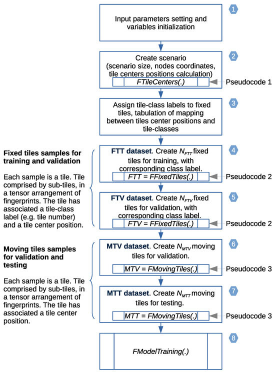
Figure 14.
Block diagram of the main execution flow of the simulator. Numbers inside hexagons represent the execution steps, these are explained in the main text.
- In step
 , the input parameters for the simulation are set, and some of the main variables that are a function of these are initialized. A list of the parameters for simulation, with the corresponding values used in our simulations, is presented in Table 9. The main variables are listed in Table 10. The number of fingerprint sources, , is fixed for the considered scenario to four fingerprint sources. The side length of the sub-tile and the number of sub-tiles per side of the tile are the two main parameters that are used in the simulations to compare the results using different sub-tile and tile sizes. The pattern-matching model is trained with initial random weights. A loop takes care to perform a number of iterations with different initial random weights, given by the parameter , as discussed in Section 5.5. The reference percentile for the selection of the best model weights with the MTV dataset is given by the parameter , discussed in Section 5.5. The parameters for the radio channel model, namely the frequency, the standard deviation in the shadow fading, and the power loss coefficient, are given by the parameters f, , and , respectively. The side length of the tile is calculated using the number of sub-tiles multiplied by the side length of the sub-tile, as indicated in Table 10, and stored in the variable . Because a tile is equivalent in size to the 2D sensor array, is the side length of the 2D sensor array. The total number of sub-tiles in a tile is stored in the variable .
Table 9. Parameters for simulation.
Table 10. Main variables for simulation.
, the input parameters for the simulation are set, and some of the main variables that are a function of these are initialized. A list of the parameters for simulation, with the corresponding values used in our simulations, is presented in Table 9. The main variables are listed in Table 10. The number of fingerprint sources, , is fixed for the considered scenario to four fingerprint sources. The side length of the sub-tile and the number of sub-tiles per side of the tile are the two main parameters that are used in the simulations to compare the results using different sub-tile and tile sizes. The pattern-matching model is trained with initial random weights. A loop takes care to perform a number of iterations with different initial random weights, given by the parameter , as discussed in Section 5.5. The reference percentile for the selection of the best model weights with the MTV dataset is given by the parameter , discussed in Section 5.5. The parameters for the radio channel model, namely the frequency, the standard deviation in the shadow fading, and the power loss coefficient, are given by the parameters f, , and , respectively. The side length of the tile is calculated using the number of sub-tiles multiplied by the side length of the sub-tile, as indicated in Table 10, and stored in the variable . Because a tile is equivalent in size to the 2D sensor array, is the side length of the 2D sensor array. The total number of sub-tiles in a tile is stored in the variable .
Table 9. Parameters for simulation.
Table 10. Main variables for simulation.
- In step, the scenario is created. The base stations’ positions (referred to as node coordinates in ) are set according to Table 7. Then, the fixed tile centers are calculated using the function (Pseudocode 1) as a function of and . The number of fixed tiles for training and validation of the datasets FTT and FTV is stored in the variables and . These are determined by the number of fixed tile batches, given through the parameter in step , and multiplied by the number of tiles that fit into the positioning area in the scenario, . In turn, is a function of the positioning area’s dimensions. The value of the variable is calculated and returned by the function . In contrast, moving tiles do not follow the grid-like pattern of the fixed tiles but are placed in random places. Therefore, the number of moving tiles in the MTV and MTT datasets is directly given through the parameters and in step .In order to present a simple and compact structure for the simulator, we avoid adding additional functions and parameters passing variables to the functions. Then, the definition of the scenario is in part distributed across the hard-coded scenario dimensions presented in the function (Pseudocode 1) and the base station positions hard-coded into the function (Pseudocode 4).
- In step
 , the fixed tile centers returned by the function are used to create a table mapping each one of the fixed tiles that covers the positioning area to the respective center positions of the tile and to a suitable class label to identify the tile. This information is used in pattern-matching method 4-MultFingIn-ClassOut, which is a classification-based method.
- In steps and , the datasets of fixed tiles FTT and FTV, introduced in Section 5.2.3, are created by calling the function (Pseudocode 2). In steps and , the moving tile datasets MTV and MTT, introduced in Section 5.2.4, are created by calling the function (Pseudocode 3).
- In step
 , the function is called. This function is in charge of implementing a selected NN structure for a given pattern-matching method and is in charge of performing the training of the NN model. For convenience and compactness in the description, this function also executes the testing phase, consisting of the actual calculation of the estimated positions for the given dataset of moving tiles for testing, MTT. In addition, the error distances for the estimated positions with the dataset MTT are calculated. This step is executed for each one of the four pattern-matching methods introduced in Table 6 (Section 4.4) independently. For simplicity, for the model training, we present the simulation flow description at a general level, suitable for use with any of the pattern-matching methods considered. Therefore, we omit defining the actual pattern-matching methods as part of the block diagram.
5.6.2. Generation of the Same Datasets of Fingerprints for the Different Pattern-Matching Methods
When comparing the results from the different pattern-matching methods, we want to avoid possible differences in the results introduced by the statistics of different datasets of fingerprints. One step toward minimizing these differences would be to increase the number of samples. However, even when enough samples are considered in the Monte Carlo methods in our simulations, we want to remove any source of variations in the results introduced by the statistics. So, it was decided that each pattern-matching method must receive the same datasets of fingerprints as input for each combination of the parameters and considered. In this way, we will compare differences in the results attributed only to the performance of each pattern-matching method.
We propose two options for how to generate the same input datasets of fingerprints for the different pattern-matching methods in the simulator. One option is to execute steps to of the main execution flow of the simulator with the same seeds in the pseudo-random number generators for each pattern-matching method. Another option is to simply execute steps to only once and store the datasets for posterior use with each one of the pattern-matching methods.
to of the main execution flow of the simulator with the same seeds in the pseudo-random number generators for each pattern-matching method. Another option is to simply execute steps to only once and store the datasets for posterior use with each one of the pattern-matching methods.It is noted that in the case of the pattern-matching method without side information, 1-SingFingIn-PosOut, not all of the fingerprints from the tile are required for pointwise estimation of the position, only the set of fingerprints corresponding to the selected reference sub-tile. In our implementation, for simplicity, we always generate the fingerprints for all of the sub-tiles in all of the tiles. The purpose of this is so that the same datasets of fingerprints can be used for all the methods. Then, for the pointwise-based method, we just use only the necessary fingerprints.
5.6.3. Execution Flow of the Model Training Function
For simplicity, the block diagram of the main execution flow of the simulator, depicted in Figure 14, does not show the individual calls to each pattern-matching method. It is assumed that step in Figure 14 is executed independently for each pattern-matching method, calling the function with the same input datasets for each method, as mentioned in the previous subsection. In our implementation, we created a tailored function for each pattern-matching method. As mentioned, for simplicity, we present the simulation flow description at the general level by describing a function that is common to all of the pattern-matching methods and thus suitable for use with any of the pattern-matching methods considered.
in Figure 14 is executed independently for each pattern-matching method, calling the function with the same input datasets for each method, as mentioned in the previous subsection. In our implementation, we created a tailored function for each pattern-matching method. As mentioned, for simplicity, we present the simulation flow description at the general level by describing a function that is common to all of the pattern-matching methods and thus suitable for use with any of the pattern-matching methods considered.A block diagram depicting the flow of the function is shown in Figure 15. Each block implements the following steps:
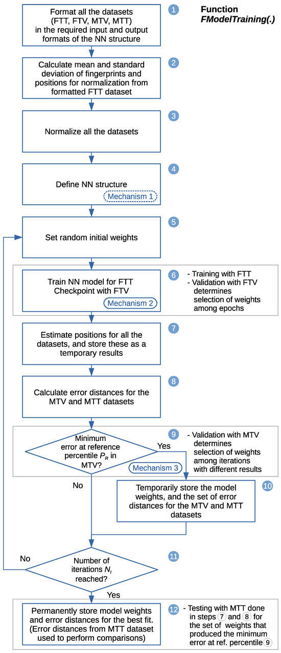
Figure 15.
Block diagram of the execution flow of the model training function . Numbers inside circles represent the execution steps, these are explained in the main text.
- In step ①, the four datasets FTT, FTV, MTV, and MTT are formatted into the input and output formats required by the NN structure implementing the selected pattern-matching method. These input and output formats are indicated in Table 6 and depicted in Figure 10, explained for each pattern-matching method in Section 4.4, and detailed in relation to the NN structures used in each pattern-matching method in Section 5.8. In the case of the pattern-matching method 4-MultFingIn-ClassOut, the output tile-classes are vectorized (e.g., using one-hot encoding).
- In step ②, the mean and standard deviation of the fingerprints and reference positions are calculated from the FTT training dataset. Then, these are used in step ③ to normalize all the datasets, shifting the values of the RSSs and positions to the zero mean, and scaling these by the inverse of the respective standard deviation. Actually, there is no need to normalize the reference positions for the fourth pattern-matching method (4-MultFingIn-ClassOut). This method is based on classification of the tile-classes. Then, for this method, the tiles are vectorized into one-hot-encoded classes.
- In step ④, the NN structure for the selected pattern-matching method is defined and introduced in the simulation process. However, the selection of the actual NN structure is decided beforehand. This is indicated by the label Mechanism 1, and shown inside a box with a dashed line, to indicate that the selection of the actual NN structure is not part of the simulation process. The selection of the NN structure is discussed in Section 5.7.1.
- In step ⑤, the random initial weights are set. This step is part of an iterative process (introduced in Section 5.5) which has the purpose of generalizing the model for moving tiles. In our simulations, the weights for each layer in the NN are set to different random initial values by calling a function provided for this purpose, taking as input a seed value. In Keras, this is achieved by retrieving the layer weight initializers, and , and setting new weights through the method for every layer in the NN model with the retrieved initializers. In each iteration of the loop for the initial random weights, all of the pseudo-random number generators are initialized with a new and unique seed (which, for convenience, in our implementation is the iteration number plus a preselected seed offset). Step ⑤ is the beginning of a loop iterating among the random initial weights for iterations, ending at step ⑪.
- In step ⑥, the training of the NN model takes place using as training data the FTT dataset of fixed tiles. The first three pattern-matching methods considered are based on regression of the position coordinates. In these methods, the target training position varies with the method. For these methods, the reference center position coordinates of the sub-tiles, returned in the data structure by the function (Pseudocode 2), are used to set the target training position. For the methods 1-SingFingIn-PosOut and 3-MultFingIn-PosOut, the position of the central sub-tile in a tile is considered the reference target training position (the selection of the central sub-tile is discussed in Section 4.4.1). For the method 2-SingFingIn-AggPosOut, the position of each one of the sub-tiles is considered the target training position. The fourth pattern-matching method, 4-MultFingIn-ClassOut, is based on classification of the tiles. In this case, the one-hot-encoded vectorization of the tile-class label is used as the training target.It is noted that in methods 1-SingFingIn-PosOut and 3-MultFingIn-PosOut, the target training position can be the same as the target reference position for the calculation of the positioning error. However, in the method 2-SingFingIn-AggPosOut, in contrast to pattern-matching methods one and three, multiple sub-tile center position estimates are aggregated. Then, the final position estimate used by us is the center of the tile, given by the aggregation performed in Equations (2) and (3). Thus, in the method 2-SingFingIn-AggPosOut, the center of the tile is used as the reference position to calculate the positioning error. In this step, the best model weights among the training epochs are selected. A checkpoint function call-back is configured to retain the weights that minimize a cost or loss metric of the model among the training epochs. The metric is evaluated using the validation dataset for fixed tiles FTV. At the end of all of the training epochs, the weights that produced the minimum metric value, among the training epochs, are retrieved and returned as the solution for the model. This process is indicated by the label Mechanism 2.
- In step ⑦, the position estimates for all of the datasets are calculated. The position estimates of the dataset of moving tiles for validation, MTV, are of importance in step ⑨ to determining the best solution among different initial weights. The position estimates of the moving tile dataset for testing, MTT, actually should be calculated after the final weights of the model are selected. However, for convenience, the position estimates of the MTT dataset are calculated at this step and stored as a temporary result. Once the final weights of the model are selected, the corresponding temporary results are returned as the final and best result of the model.The first three pattern-matching methods are based on regression. These return a normalized position estimate for each input set or vector of fingerprints. In the case of the method 2-SingFingIn-AggPosOut, the output position estimates are aggregated (as discussed in Section 4.4.2) to produce a final position estimate. Then, in the first three pattern-matching methods, the output position estimate for each input set or vector of fingerprints is unnormalized. The fourth method, 4-MultFingIn-ClassOut, returns a vector of tile-class probabilities. In this case, the position is estimated as explained in Section 4.4.4, that is, calculated from the output tile-class probabilities and the mapping between the tile-classes and the center coordinates of the tiles.It is noted that the model was trained for fixed tiles. Then, when it is used with the moving tiles of the MTV and MTT datasets, this can be interpreted as a transfer learning approach. However, the final selection of the model is biased by the action performed in step ⑨, selecting the best model among the different initial weights by evaluating the error distance in the moving tiles for the validation, MTV, dataset.
- In step ⑧, the error distances are calculated for the MTV and MTT datasets, using unnormalized positions, with Equation (1). Here, Equation (1) takes as input the estimated position coordinates and the known ground truth reference position coordinates. In the methods 1-SingFingIn-PosOut and 3-MultFingIn-PosOut, the ground truth reference position coordinates are taken from the position of the tile which was defined as the center position of the central sub-tile (as discussed in Section 4.4.1). The reference center position coordinates of the sub-tiles are returned in the data structure by the functions and . In the pattern-matching methods 2-SingFingIn-AggPosOut and 4-MultFingIn-ClassOut, the ground truth reference position is the center of the tile. This is consistent with the final position estimate in these methods calculated from the aggregated sub-tile position estimates using Equations (2) and (3) in method two and from the mapping from the tile-class labels to the center positions of the fixed tiles using Equations (4) and (5) in method four.
- In step ⑨, the Cumulative Density Function (CDF) of the error distances resulting from the MTV dataset is calculated. This step is part of the iterative process of generalizing the model for moving tiles (introduced in Section 5.5). The goal is to select the model that generalizes best for moving tiles by selecting the model that minimizes the 95th percentile of the CDF of the error distances for all of the moving tiles in the MTV dataset among the model training iterations initiated with different random weights.In the first iteration of the loop started in step ⑤, the value of the error distance at the 95th reference percentile, , of the CDF is retained as the minimum error, and the error distances and model weights for this iteration are temporarily stored and kept as the best model in step ⑩. From the second iteration onward, the error distance at the 95th reference percentile is compared against the minimum error obtained in a previous iteration. If the error distance at this percentile is smaller than the minimum error obtained in a previous iteration, this value is retained as the minimum, and the error distances and model weights for the current iteration are temporarily stored and kept as the best model in step ⑩. The training process is repeated again, with different random initial weights, repeating the process from step ⑤ until the number of iterations (given in Table 9) is completed. The number of iterations is checked with the condition of step ⑪. For convenience, in step ⑩, the error distances obtained from the testing dataset of moving tiles, MTT, are also temporarily stored. The process described above is indicated by the label Mechanism 3.
- Finally, in step ⑫, the model weights that produced the smallest error distance at the given CDF percentile are kept as the best and final weights for the model. The best weights are used to calculate the error distances in the testing dataset of moving tiles, MTT. Actually, for convenience, the estimation of the positions and calculation of the error distances for the MTT dataset are carried out in steps ⑦ and ⑧, and the best results, along with the corresponding weights, are temporarily stored in step ⑩. In addition, the error distances resulting from the MTT dataset using the best weights are permanently stored in step ⑫ to perform later comparisons among the other pattern-matching methods and among different tile arrangements (introduced in Section 5.9). The details of the settings for each pattern-matching method are detailed in Section 5.8, and the results obtained are presented in the next section.
5.7. Mechanisms to Optimize the Models and Minimize the Error Distance
We benchmark different patternmatching methods using different kinds of input data arrangements and using different NN structures (also referred to as NN architectures by some authors), namely feedforward and convolutional. The challenge is to find a suitable NN that generalizes for each pattern-matching method. Simply making the NN bigger is not necessarily a solution, as the NN tends to overfit.
When training an NN model, there is no guarantee of obtaining the best fit. An NN may look unsuitable just because there were not enough training epochs or the optimization algorithm became stuck in local minima. In this latter case, the model may have been trained with a set of initial weights that produced a solution worse than that which could have been obtained with another set of initial weights. This is a problem when benchmarking NNs for selecting the best model. The challenge is how to select the most suitable NN structure for each pattern-matching method so that the fit is optimized to return a minimum error distance, minimizing the probability of bad fits.
Given the non-convex problem to be solved and the infinite possibilities in terms of how to construct an NN, we cannot guarantee that we are delivering the best result that could be obtained for each one of the proposed pattern-matching methods. However, when selecting the NN structure for each pattern-matching method and when calculating the results, we do our best to aim for a solution that minimizes the positioning error with the approaches discussed below.
We use the word mechanism to give a name to the different approaches that are used to optimize the model adopted in a pattern-matching method so it can deliver results with a minimum positioning error. Three mechanisms are considered, acting at different levels, ranging from the selection of the NN structure to the repetition of the training with different initial weights. The mechanisms considered are as follows:
- 1.
- Selection of the NN structure.
- The goal is to select a suitable NN structure such that the model can deliver results with a minimum positioning error when compared to models implementing other NN structures.
- 2.
- Selection of the best model weights among training epochs.
- The goal is to select the model weights that minimize the positioning error, generalizing the model for fixed tiles.
- 3.
- Selection of the best weights among model training iterations with different initial random weights.
- The goal is to select the model weights that minimize the positioning error, generalizing the model for moving tiles.
5.7.1. Mechanism 1: Selection of the NN Structure
The first mechanism consists of the selection of the structure of the NN. The goal is to select a suitable NN structure such that the model can deliver results with a minimum positioning error. In this regard, we tested a number of NN structures to determine those to be used in each pattern-matching method. The selection of the NN structures was carried out using two tile arrangements (introduced in Section 5.9) for evaluation. The first tile arrangement uses and mm. The second tile arrangement uses and mm.
The simulation process presented in Section 5.6 was executed for each one of the four pattern-matching methods, with different NN structures and using the two selected tile arrangements, for at least 200 different sets of random initial weights. We kept the best result in each case, measured by the minimum error distance at the 95th percentile ( cut) of the CDF of the error distances resulting from the MTV dataset.
Actually, for the method 1SingFingInPosOut, we considered the error distances resulting from all of the sub-tiles in the whole positioning area on the basis that there were more pointwise samples contributing to the statistics. For the method 2-SingFingIn-AggPosOut, we did not compute the aggregation of the estimated position results. In this particular case, the method 2-SingFingIn-AggPosOut is equivalent to executing the method 1-SingFingIn-PosOut considering all of the sub-tiles in the whole positioning area. The rationale is that if we select an optimal NN structure considering the minimization of the error distances for all of the sub-tiles in the whole positioning area, any possible enhancement in minimizing the positioning error attained from the aggregation of the results (positions) in the method 2-SingFingIn-AggPosOut is independent of the selection of the NN structure. Therefore, we selected the same NN structure for the methods 1SingFingInPosOut and 2SingFingIn-AggPosOut.
For each pattern-matching method and tile arrangement, we tested different NN structures by changing the activation functions, the number of layers, and layer width in a quest to find the NN structure that minimized the error distance. Initially, we searched for an optimal NN structure through systematic experimentation with a grid search [210]. Then, from the best NN structure found by the grid search, we tested making corrections by changing the NN structure as a function of the results observed. In the case of the FFNNs, we observed that adding more layers or increasing their width resulted either in overfitting or in larger error distances in the estimated position results. After several cycles of changing the NN structure, we found the suitable the NN structures shown in the next subsection. In the actual process, we tested the lighter pattern-matching methods many more times, and with many more combinations in the NN structure, than the heavier ones, in the order 1-SingFingIn-PosOut, 3-MultFingIn-PosOut, and 4-MultFingIn-ClassOut. This approach was carried out in an attempt to minimize the possibility of not identifying a case in which a lightweight method could perform as well as a heavier one. It is noted that this process was carried out only in the tests with the two tile arrangements mentioned above. The best-performing NN structures found from these tests were reused for different tile arrangements in the benchmark tests that follow.
Mechanism 1 is shown in step ④ of the block diagram describing the model training execution flow, in Figure 15. It is noted that in the block diagram, Mechanism 1 appears with a label drawn with a dashed line. This is to distinguish that Mechanism 1 is not programmed as part of the simulation process for the final benchmarking of all of the pattern-matching methods and tile arrangements considered. Instead, Mechanism 1 comprises a process that requires the execution of independent simulations several times to tune the NN structures, according to the results observed in previous simulations. This process is not presented as part of the simulation process in the diagram. In contrast, Mechanisms 2 and 3 are actually programmed as part of the simulation process. Mechanisms 2 and 3 react in real time during the execution of the simulation to find the value of the weights that minimizes the selected optimization metric of the model.
We carried out extensive simulations with different NN structures and sets of hyperparameters; however, we cannot guarantee that the NN structures that we found (presented in the next subsection) are the best ones that exist. The NN structures reported are the best that we were able to find. However, we explain next that the NN structure found for the pattern-matching methods 1SingFingInPosOut and 2SingFingInAggPosOut is suitable and enough to show that the positioning error decreases when introducing spatial side information, independently of the existence of a better-performing NN structure. To explain the reasoning, we need to anticipate from the results presented in Section 6 that the pattern-matching method 2SingFingInAggPosOut performs better than the method 1SingFingInPosOut. Therefore, there is a gain in terms of minimizing the error distance when using spatial side information.
Pattern-matching methods 1SingFingInPosOut and 2SingFingInAggPosOut implement the same NN structure. The method 2SingFingInAggPosOut can be interpreted as the execution of the method 1SingFingInPosOut times for all of the sensors in the 2D sensor array (or sub-tiles in the tile), as discussed in Section 4.4.2. Then, the gain observed with the method 2SingFingInAggPosOut is attributed to the aggregation of position estimates, and in this case, it is independent of the selected NN. That is, the gain comes from the contribution of the spatial side information. If there is an NN structure for the method 1SingFingInPosOut that produces a better result than that presented here, then it is expected that in the aggregation process of the method 2SingFingInAggPosOut, the result will be also better than that presented here. Thus, if there are enhancements introduced by the selected NN structure, the end result showing that there is a gain with spatial side information does not change. With the NN structure found by us, we can come to the conclusion confirming that spatial side information contributes to a gain in terms of minimizing the positioning error.
5.7.2. Mechanism 2: Selection of the Best Model Weights Among Training Epochs
Mechanism 2 consists of the selection of the best model weights among the training epochs. The goal is to select the model weights that minimize the positioning error, generalizing the model for fixed tiles. This is achieved using a checkpoint call-back function that retains the weights for the best optimization metric found among the epochs. The weights for the best value obtained of the selected optimization metric are retrieved at the end of all of the training epochs.
This mechanism is explained in step ⑥ of the block diagram describing the model training execution flow in Section 5.6.3 and depicted in Figure 15.
5.7.3. Mechanism 3: Selection of the Best Model Weights with Different Initial Weights
Mechanism 3 consists of the selection of the best model weights among the model training iterations with different initial random weights. The goal is to select the model weights that minimize the positioning error, generalizing the model for moving tiles. The training process is repeated with different initial random weights for a number of iterations. Then, the set of weights that produced the minimum error distance at the 95th percentile ( cut) of the CDF of the error distances resulting from the MTV dataset is kept as the best model.
This mechanism is explained in step ⑨ of the block diagram describing the model training execution flow in Section 5.6.3 and depicted in Figure 15.
5.8. NN Structure for Each Pattern-Matching Method and Model Training Details
The NN structure for each pattern-matching method and the model training details are presented in the subsections that follow. We consider the activation functions part of the NN structure.
5.8.1. NN Structure for Methods 1SingFingInPosOut and 2SingFingInAggPosOut
Pattern-matching methods 1-SingFingIn-PosOut and 2-SingFingIn-AggPosOut implement the same NN structure. The mapping from the fingerprints to the position coordinates is solved as a regression problem. The NN structure consists of an FFNN with inputs, with one for each fingerprint, and two outputs for the estimated position coordinates. The pattern-matching methods are explained in Section 4.4.1 and Section 4.4.2 and summarized in Table 6 (Section 4.4).
Pattern-matching methods 1-SingFingIn-PosOut and 2-SingFingIn-AggPosOut implement the FFNN shown in Table 11. The model is trained with the Root Mean Square propagation (RMSprop) optimizer, with a Mean Absolute Error (MAE) cost (loss) function. The RMSprop optimizer performs the optimization in the training of the model with an adaptive learning rate.
Table 11.
FFNN for pattern-matching methods 1-SingFingIn-PosOut and 2-SingFingIn-AggPosOut.
5.8.2. NN Structure for Pattern-Matching Method 3-MultFingIn-PosOut
In pattern-matching method 3-MultFingIn-PosOut, the mapping from the fingerprints to the position coordinates is solved as a regression problem. The NN structure consists of an FFNN with inputs, with one for each fingerprint from each sensor in the 2D sensor array, and two outputs for the estimated position coordinates. The pattern-matching method is explained in Section 4.4.3 and summarized in Table 6 (Section 4.4).
Pattern-matching method 3-MultFingIn-PosOut implements the FFNN shown in Table 12. The model is trained with the RMSprop optimizer, with a MAE cost function. The RMSprop optimizer performs the optimization in the training of the model with an adaptive learning rate.
Table 12.
FFNN for pattern-matching method 3-MultFingIn-PosOut.
5.8.3. NN Structure for Pattern-Matching Method 4-MultFingIn-ClassOut
In pattern-matching method 4-MultFingIn-ClassOut, the mapping from the fingerprints to the position coordinates is solved as a classification problem. The NN structure consists of a 2D CNN with inputs, with one for each fingerprint from each sensor in the 2D sensor array. The NN has outputs, with the purpose of mapping the inputs to a classification among tile-classes, expressed as a likelihood probability. The patternmatching method is explained in Section 4.4.4 and summarized in Table 6 (Section 4.4).
Pattern-matching method 4-MultFingIn-ClassOut implements the 2D CNN shown in Table 13. From Mechanism 1 (Section 5.7.1), we found that it was not necessary to use pooling layers. A softmax activation function is used in the last layer to implement multi-class classification. The model is trained using the RMSprop optimizer, with a categorical cross-entropy cost function. The RMSprop optimizer performs the optimization in the training of the model with an adaptive learning rate.
Table 13.
CNN for pattern-matching method 4-MultFingIn-ClassOut.
5.8.4. Notes on the Model Training Hyperparameters
All of the models were trained with the RMSprop optimizer and an adaptive learning rate. A maximum number of 100 training epochs was selected for the three pattern-matching methods based on regression (1SingFingInPosOut, 2SingFingInAggPosOut, and 3MultFingInPosOut), and 40 training epochs were selected for the pattern-matching method based on classification (4-MultFingIn-ClassOut). Observing the loss metric in the validation dataset for fixed tiles, FTV, we noticed that before reaching the selected maximum number of epochs, the loss metric either reached a minimum value or showed a trend with oscillations around a possible minimum value. We recall that the training is carried out times with different initial random weights (as explained in Section 5.6.3).
The batch sizes were determined through systematic experimentation when searching for an optimal NN structure in Mechanism 1 (Section 5.7.1). We recall that the models are trained with fixed tiles; however, in the end, they must generalize for moving tiles. A better generalization was observed, with smaller positioning errors, when adopting small batch sizes, particularly in the order of 32 data samples. The same observation has been reported in the literature, which discusses the degradation of the model’s generalization when increasing the batch size [224]. Thus, the training of the models for all of the pattern-matching methods was carried out using batch sizes of 32 data samples.
5.9. Execution of the Simulations
The inter-antenna spacing in phased-array antennas is typically half-wavelength. In simple phased-array antennas, the typical element spacing is optimized to the half-wavelength to deal with grating lobes [225,226,227]. This may be the case if this kind of antenna is repurposed as a 2D sensor array. However, irrespective of the requirements for communication purposes, it remains to be studied whether the antenna spacing can be exploited to obtain distinctive signal patterns that benefit fingerprinting-based positioning. In this study, we do not claim that the 2D sensor array has to be a phased-array antenna. Therefore, we relax the constraint on the half-wavelength inter-antenna spacing. However, we keep the antenna spacing close to the half-wavelength in a set of one of the cases considered below.
In addition, we do not consider the actual antenna design aspects related to the construction of the 2D sensor array. In this context, we are working only with the numeric modules of what would be the equivalent of the RSSs, ignoring the phases and AoA.
For a frequency of GHz, the half-wavelength is approximately mm. In the simulations, we consider an inter-sub-tile spacing that is in the same order of the half-wavelength of GHz, but it is not exactly half-wavelength. We choose to initially work with an inter-sub-tile spacing given by mm and mm, which bounds the mm half-wavelength. In addition, we work with an inter-sub-tile spacing given by mm in order to explore the results for a smaller 2D sensor array.
We note that in the radio channel model, Equation (7), the frequency contributes to a linear attenuation of the radio signal (in the dB domain). This attenuation is constant for a fixed frequency; therefore, it disappears when normalizing the datasets to the zero mean scaled by the standard deviation. This means that varying the frequency does not change the numeric value of the results in this study. Therefore, the channel model can be thought of as suitable for other frequencies but limited to scenarios with the same power loss coefficient and shadow fading characteristics. In this context, the results could be generalized to the widely used frequency of GHz for scenarios with the same characteristics. The half-wavelength of GHz is mm, which is close to the inter-sub-tile distances considered.
Simulations are carried out for different combinations of the parameters (the side length of the sub-tile) and (the number of sub-tiles per side of the tile), executing the simulation flow presented in Section 5.6. The selected combinations of and are listed in Table 14. The combinations of and define different tile sizes, and are referred to as tile arrangements. The table also lists the total number of tiles required to cover the positioning area, , obtained from the function (Pseudocode 1), and the number of NN parameters for each pattern-matching method, which are returned by the machine learning library for the selected NN structure.
Table 14.
Tile arrangements.
The associations between each pattern-matching method and the corresponding NN structure are provided in Section 5.8, and these are summarized in Table 6 (Section 4.4).
Simulations are carried out for each one of the tile arrangements listed in Table 14, and for each one of the four pattern-matching methods. The comparison of the results for each tile arrangement and pattern-matching method is presented in the next section.
It is out of the scope of this article to evaluate the computing cost of each pattern-matching method. However, the number of NN parameters for each method and tile arrangement is provided in Table 14 to report the dimensions of the problem to be solved. Note that in the case of pattern-matching method 2-SingFingIn-AggPosOut, there is an additional computing overhead. Actually, in this method, instances of the NN model implemented need to be executed, with one for each sub-tile.
5.10. Consistency in the Comparison of the Results Among Scenarios with Different Tile Sizes
To obtain a consistent comparison among scenarios with different tile sizes, we need to look at the consequences resulting from varying the 2D sensor array’s size and, correspondingly, the tile size. The challenge is how to make consistent comparisons of the results among scenarios using different tile sizes.
From one perspective, the tiling process produces, in some cases, for some tile sizes, an untiled stripe adjacent to the top and/or the right borders of the area intended for positioning. We recall that the tiling is carried out by starting to tile the scenario from one border to the opposite border using entire tiles. An untiled stripe occurs in cases in which the dimensions of the area intended for positioning (13,000 mm × 5000 mm) are not a multiple of the side length of the tile. So, for some tile sizes, it is not possible to entirely fill the area intended for positioning from one border to the opposite border using entire tiles, as explained in Section 5.3. We recall that the actual area of the scenario used for positioning is determined by the grid of fixed tiles constructed in the tiling process, through the execution of the function (Pseudocode 1). As a consequence, the tested scenarios do not all have exactly the same positioning area and do not all have the same density of samples close to the borders. In this regard, it is unclear at this point whether the distribution of the positioning errors for these cases will be slightly different to what could be obtained if an exact number of tiles fitted into the dimensions of the area intended for positioning (or, in other words, to the case in which the tiles cover the area intended for positioning entirely).
From another perspective, the size of the 2D sensor array, and hence the tile, limits the useful area in which positioning can be performed. A position is associated with one point of the 2D sensor array—for example, the center of the tile. Bigger tile sizes do not have the resolution for performing positioning as close to the borders as smaller tiles do. In this context, smaller 2D sensor arrays, and correspondingly the tiles associated with them, will delimit a positioning area of a bigger size than the area delimited by bigger 2D sensor arrays.
All in all, changing the size of the tile causes variations in the useful area of the scenario for performing the positioning, and this causes inconsistencies in the comparison of scenarios with different tile sizes. These inconsistencies are in the sense that we are not strictly using the same positioning area among different tile arrangements to compare the results, and that the density of samples close to the borders is different for different tile sizes.
While it would be possible to make corrections to theoretically normalize all of the cases for a consistent comparison, in the sense of keeping a constant distance to the borders of the scenario for any tile arrangement, we instead adopt a pragmatic approach that represents the case of selecting a 2D sensor array of a given size in a real scenario. In this context, these inconsistencies are regarded as consequences resulting from the use of different tile sizes in the discretization of the positioning area. These consequences are proper to the arrangement considered. Then, certainly, the size of the 2D sensor array will affect how close to the borders we can perform the positioning, affect the size of the positioning area, and result in an uncovered area close to the borders in some cases. For the purpose of determining whether the use of spatial side information helps to reduce the positioning error, these inconsistencies are negligible. This observation is based on the results obtained, comparing the operating regions of the positioning errors for the different pattern-matching methods, and considering the effect of the samples close to the borders, as discussed in Section 6. For other purposes, these inconsistencies should be regarded as trade-offs to add to the list of trade-offs comprising cost, size, intended use, etc., which must be evaluated altogether for a desired operating point of performance. These aspects fall outside of the scope of our current study.
5.11. Software and Hardware Details
The simulator was implemented in the Python 3 programming language, using the machine learning library TensorFlow [228], version 2.4.2, and the Keras library, version 2.4.0. Each simulation was executed in a single core of a multi-core CPU (Central Processing Unit) with a 3.2 GHz clock frequency, a 512 KiB cache size, and 128 GiB of CPU RAM (Random-Access Memory). A GPU (Graphics Processing Unit) with 24 GiB of memory, a 1395 MHz clock frequency, and 10496 shading units was used to process the NN models.
6. Results of the Simulations
In the simulations, the four pattern-matching methods described in Section 4 receive exactly the same input datasets of fingerprints for each tile arrangement (combination of the parameters and , introduced in Section 5.9) considered. So, the results obtained represent the capability of the method to estimate the position, along with the possible limitations due to improper selection of the NN model or due to non-optimal training of the NN model, for the system and assumptions considered. To minimize the effects of these limitations, we applied the mechanisms discussed in Section 5.7.
Positioning performance is measured according to the positioning error distance, calculated using Equation (1). The error distances are calculated for all of the moving tiles in the MTT dataset in step ⑧ in the block diagram describing the model training execution flow (Section 5.6.3, Figure 15) for each one of the four pattern-matching methods and for all the tile arrangements given in Table 14. The error distances for all of the moving tiles of the MTT dataset are presented with a CDF for posterior comparison against the other pattern-matching methods and tile arrangements. In the results, we represent with CDF the CDF of the error distances e corresponding to the given case, that is, pattern-matching-method, number of sub-tiles per side of the tile, and side length of the sub-tile.
The subsections that follow summarize the results of the simulations. First, the error distance is calculated for trivial solutions, as an initial reference for benchmarking all of the pattern-matching methods. Next, the results are presented for each pattern-matching method, for all of the tile sizes given by the tile arrangements considered. The tile arrangements are divided into three groups, arranged by the three side lengths of the sub-tiles considered, , as summarized in Table 14. The different numbers of sub-tiles per side of the tile considered, , are listed in the table. Given that there is a total number of 32 combinations of sub-tile sizes and numbers of sub-tiles per side of the tile, for simplicity and in order to summarize several results in a few figures, we work initially with a few cuts at different percentiles in the CDFs of the error distances. For the most notable and best results observed, we will work with the full CDF of the error distances. Finally, the results between the pattern-matching methods are compared; the particular details of the errors for the method 4-MultFingIn-ClassOut are discussed; different observations from the results for the cases with spatial side information and aggregation in the fingerprint domain are summarized; and information about the computing costs and the reproducibility of the results is provided.
6.1. Baseline Reference Performance
The positioning error, in terms of the error distance, is calculated as a baseline reference for two trivial solutions. Any pattern-matching method must perform better than the trivial solutions. First, a trivial pattern-matching method is considered that returns as the position estimate the center coordinates of the positioning area ( m, m), for any input vector of fingerprints. It is assumed here that the positioning area is equal to the area intended for positioning. Second, a trivial pattern-matching method that returns as the position estimate a random position drawn from a uniform distribution in the interval of each coordinate in a positioning area equal to the area intended for positioning is considered. The positioning error results for these baseline reference solutions are shown in Figure 16. This figure also includes the positioning error for the case with no side information. The results for this case were obtained by fingerprinting using pointwise samples, applying the pattern-matching method 1-SingFingIn-PosOut (discussed below). It is observed that fingerprinting with pointwise samples performs better than the trivial baseline cases, with a smaller error distance at each percentile. Fingerprinting using pointwise samples (with no side information) with the pattern-matching method 1-SingFingIn-PosOut is the performance to beat. Next, we focus on studying whether the pattern-matching methods with side information can perform better than fingerprinting using pointwise samples.
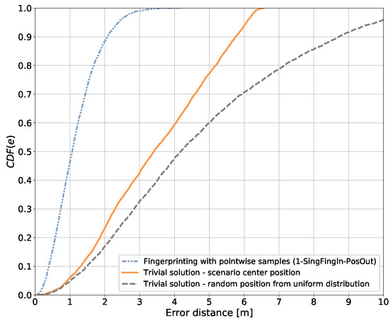
Figure 16.
Baseline reference performance of the error distance in two trivial solutions and comparison to the error distance obtained with the fingerprinting method based on pointwise samples (pattern-matching method 1-SingFingIn-PosOut). CDF is the Cumulative Distribution Function (CDF) of the error distances e corresponding to each case.
6.2. Results with Pattern-Matching Method 1-SingFingIn-PosOut
The smaller the size of the tile, the higher the number of tiles that are required to cover the whole positioning area, and the higher the number of positions that are sampled. The size of the tile is determined by the number of sub-tiles per side of the tile, , and the side length of the sub-tile, .
Pattern-matching 1-SingFingIn-PosOut does not exploit side information. It takes a pointwise sample of the fingerprints from one sub-tile in the whole tile. So, it would be expected that in varying the size of the tile, the statistics of the positioning error will not change. However, the smaller the size of the tile, the higher the number of samples in the whole positioning area that contribute to the statistics.
The CDF of the error distances obtained using the MTT dataset, from the simulations with this pattern-matching method, for a given tile arrangement (that is, a given sub-tile size and number of sub-tiles per side of the tile) is calculated. Then, the CDF is cut at different percentiles. The error distances resulting from the cuts in the CDFs of the error distances at different percentiles are plotted for each number of sub-tiles considered, , in the three subfigures in Figure 17. Each subfigure groups the results for each one of the three selected side lengths of the sub-tiles, . The results for all of the considered are linked with a distinctive line for each percentile cut.
It is observed in Figure 17 that, ignoring minor variations, there is a trend in which the error distance seems constant for all numbers of sub-tiles and sizes of the sub-tiles considered. In fact, we expect these results to be constant for any number of sub-tiles and sub-tile sizes. As explained above, in reducing the size of the sub-tiles and the number of sub-tiles per tile, a higher density of samples is obtained (that is, a higher number of tiles) than when increasing the size of the sub-tiles and the number of sub-tiles per tile. Nevertheless, the statistics should not change when varying these parameters. Thus, ideally, the cuts in the CDF of the error distances at different percentiles, for all cases considered, should appear as horizontal lines. However, in practice, the bigger the size of the tiles, the smaller the number of samples that contribute to the statistics. Therefore, the results observed may be the result of the statistics. In addition, we may observe the possible non-optimal training of the NN model for this method, as discussed in Section 5.7.
From the comparisons of the results obtained using the method 1-SingFingIn-PosOut, we take the results for the tile arrangement with and mm as a reference for comparison against the other pattern-matching methods. The complete CDF for this pattern-matching method and the selected reference tile arrangement is shown in Figure 16 and in the figures presented in Section 6.6.1 and Section 6.6.2.
6.3. Results with Pattern-Matching Method 2-SingFingIn-AggPosOut
The positioning results obtained with pattern-matching method 2SingFingInAggPosOut and different tile arrangements are shown in the three subfigures of Figure 18. Each subfigure groups the results for each one of the three selected side lengths of the sub-tiles, . Each subfigure shows the error distances from the cuts in the CDFs of the error distances at different percentiles for all of the sub-tiles per side of the tile considered for the given . The results for all of the considered are linked with a distinctive line for each percentile cut. Looking at the 95th percentile in each subfigure, it is observed that increasing the number of sub-tiles per tile reduces the error distance. In this method, the trend shows that in the interval of the number of sub-tiles considered, the greater the spatial side information, the smaller the error distance. We did not calculate any results beyond , so it is unknown whether this trend continues or whether it reaches a minimum for a certain number of sub-tiles. However, for the scenario considered, bigger tiles are not of much interest to practical applications, and in addition, we observe later that other methods perform better than this one. Therefore, we do not investigate how the error distance varies for bigger tile sizes.
The minima at the 95th percentile for the interval of considered are indicated using red circles in Figure 18. These occur at the following values:
- sub-tiles per side of the tile, for mm;
- sub-tiles per side of the tile, for mm;
- sub-tiles per side of the tile, for mm.
In the case of mm, the minimum error is at , in contrast to for the other two cases. Either we did not find a good representative result with a minimum error for or there is effectively a minimum for .
Varying the side length of the sub-tiles and comparing the error distances at the 95th percentile, we observe that the bigger the sub-tile size, the smaller the error distance. For example, the error for mm with is close to m, whereas the error for mm with is close to m. One hypothesis for this behavior is based on the fact that there are more samples contributing to a better estimation of the position. However, this may be not the case, as in the cases with and , both have a minimum error with the same number of samples (the same number of sub-tiles per side of the tile, ); however, the latter has a smaller minimum error distance than the former. Yet, another hypothesis can be formulated in the sense that the bigger the sub-tile size, the further apart the fingerprints are located from each sub-tile; thus, it would be possible to obtain more distinctive patterns of fingerprints for estimating a position with less error. The pattern-matching methods that follow present more interesting results, so we did not study this method further.
6.4. Results with Pattern-Matching Method 3-MultFingIn-PosOut
The positioning results obtained with pattern-matching method 3MultFingInPosOut and different tile arrangements are shown in the three subfigures of Figure 19. Each subfigure groups the results for each one of the three selected side lengths of the sub-tiles, . Each subfigure shows the error distances from the cuts in the CDFs of the error distances at different percentiles for all of the sub-tiles per side of the tile considered for the given . The results for all of the considered are linked with a distinctive line for each percentile cut. Looking at the 95th percentile in each subfigure, it is observed that starting from a small tile (composed of a small number of sub-tiles), increasing the number of sub-tiles reduces the error distance. However, this trend reverses after a certain number of sub-tiles, which we call the best . The error distance starts to grow after the best when increasing the number of sub-tiles further.
One hypothesis about the best is that when increasing the number of sub-tiles, there is more information for determining the position more accurately, which results in minimization of the error distance. However, on increasing the number of sub-tiles too much, or their size, the size of the tile increases, and the inter-tile distance increases (hence, fewer tiles are required to cover the whole scenario). This contributes to fewer labeled samples in the training phase, meaning a lower number of trained positions with sparser reference positions from the fixed tiles. Thus, the NN has a smaller density of reference positions for interpolating the position of a moving tile. So, the greater the number of sub-tiles, the bigger the tile, the longer the inter-tile distance, the fewer the number of tiles and training points in the scenario, and the coarser the resolution for estimating the positions.
Related to sparser reference positions, we recall that training is performed using the reference (center) positions of fixed tiles. From the perspective of ideally limiting the NN to returning as the estimated position the center of the nearest fixed tile, the longer the inter-tile distance, the higher the error in the estimated position. In practice, the NN may return an estimated position calculated mainly from the nearest fixed tile centers; thus, the longer the inter-tile distance, the higher the error in estimating the position of the moving tile.
Another hypothesis about the best is that in this method, we are adjusting the size of the first layer of the NN according to the number of sub-tiles. However, we keep a constant size in the intermediate layers and a constant number of layers for all of the tile arrangements. So, we cannot discard the possibility that the NN has a lower representational capacity when increasing the number of sub-tiles.
The hypotheses above may contribute to decreasing the resolution for estimating the position when the number of sub-tiles increases above the observed best .
The minima at the 95th percentile are indicated using red circles in Figure 19. These occur at the following best , for each :
- sub-tiles per side of the tile, for mm;
- sub-tiles per side of the tile, for mm;
- sub-tiles per side of the tile, for mm.
Varying the side length of the sub-tiles, , and comparing the error distances at the 95th percentile, we observe that the smaller the sub-tile size, the smaller the error distance. For example, the error for mm with is below m, whereas the error for mm with is above m.
Comparing the minima at the 95th percentile, as listed above, we observe that the smaller the tile (and 2D sensor array), the smaller the error distance given that for mm, the side length of the tile (2D sensor array) is mm mm, and for mm, the side length of the tile (2D sensor array) is mm mm.
As a summary of this method, we learn that there is an optimal size of the tile (and hence the 2D sensor array) that minimizes the error distance.
6.5. Results with Pattern-Matching Method 4-MultFingIn-ClassOut
The positioning results obtained with pattern-matching method 4MultFingInClassOut and different tile arrangements are shown in the three subfigures of Figure 20. Each subfigure groups the results for each one of the three selected side lengths of the sub-tiles, . Each subfigure shows the error distances from the cuts in the CDFs of the error distances at different percentiles for all of the sub-tiles per side of the tile considered for the given . The results for all of the considered are linked with a distinctive line for each percentile cut. Looking at the 95th percentile in each subfigure, a result similar to that for the method 3-MultFingIn-PosOut is observed. Starting from a small tile (composed of a small number of sub-tiles), increasing the number of sub-tiles reduces the error distance. However, this trend reverses after a certain number of sub-tiles, which we call the best . The error distance starts to grow after the best when increasing the number of sub-tiles further.
In this method, the training is performed using a given number of tile-classes, which is determined by the number of tiles that covers the positioning area in the scenario. The total number of tiles in the scenario is a function of the size of the tiles. The size of the tiles is given by the number of sub-tiles per tile (i.e., a function of the number of sub-tiles per side of the tile, ) and by the sub-tile sizes (i.e., a function of the side lengths of the sub-tiles, ).
As with the previous method, the reasoning is that increasing the number of sub-tiles brings more information for determining the position more accurately, which results in a reduction in the error distance. However, on increasing the number of sub-tiles too much, or their size, the size of the tiles increases, the inter-tile distance increases, the number of tiles required to cover the whole positioning area decreases, and the number of tile-classes decreases. Because the estimated position of the moving tile is calculated from the weighted contributions of the center positions of the fixed tiles, it follows the hypothesis that the bigger the tile, the coarser the resolution for estimating the position. So, after a certain tile size, the performance starts to degrade. As a summary, it is hypothesized that the gains attained by increasing the number of sub-tiles are traded off by a coarser resolution of the reference points used to estimate the position. The coarser resolution is a consequence of the increment in the size of the tiles and the associated reduction in the density of tiles in the positioning area.
The minima at the 95th percentile are indicated using red circles in Figure 20. These occur at the following best for each :
- sub-tiles per side of the tile, for mm;
- sub-tiles per side of the tile, for mm;
- sub-tiles per side of the tile, for mm.
Varying the side length of the sub-tiles, , and comparing the error distance at the 95th percentile, we observe that the smaller the sub-tile size, the smaller the error distance. For example, the error for mm with is close to m, whereas the error for mm with is close to m.
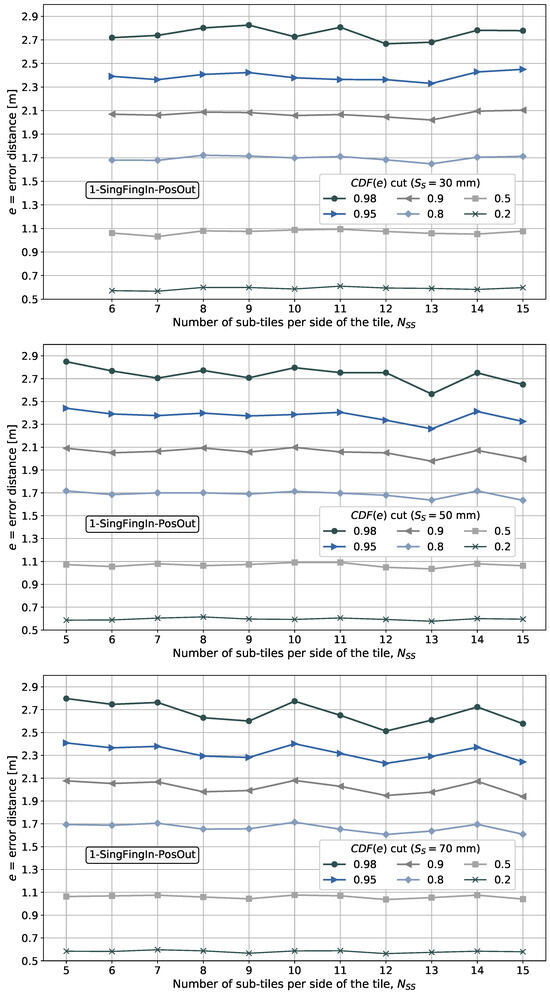
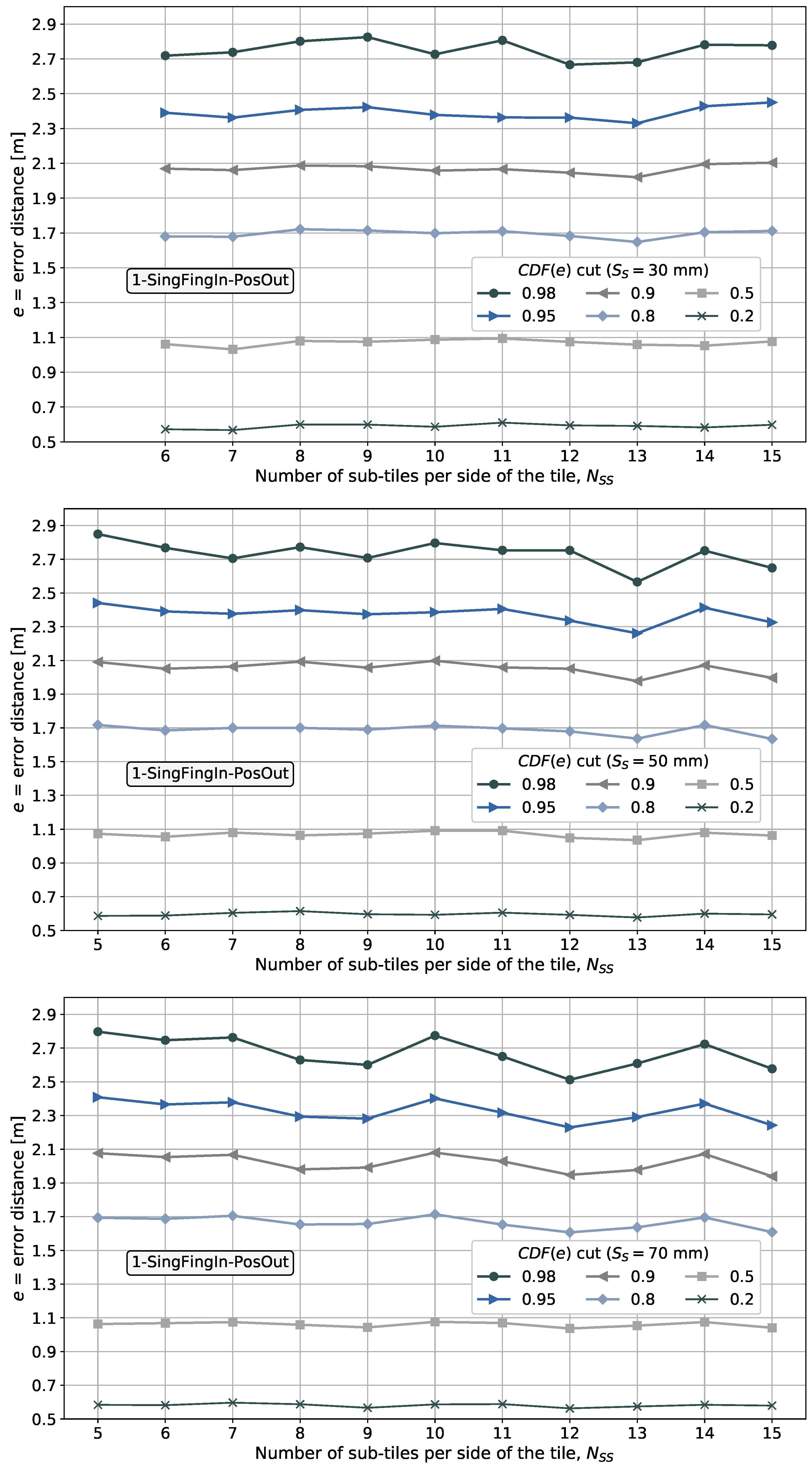
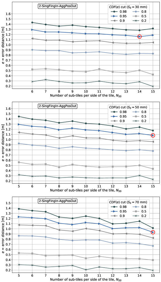
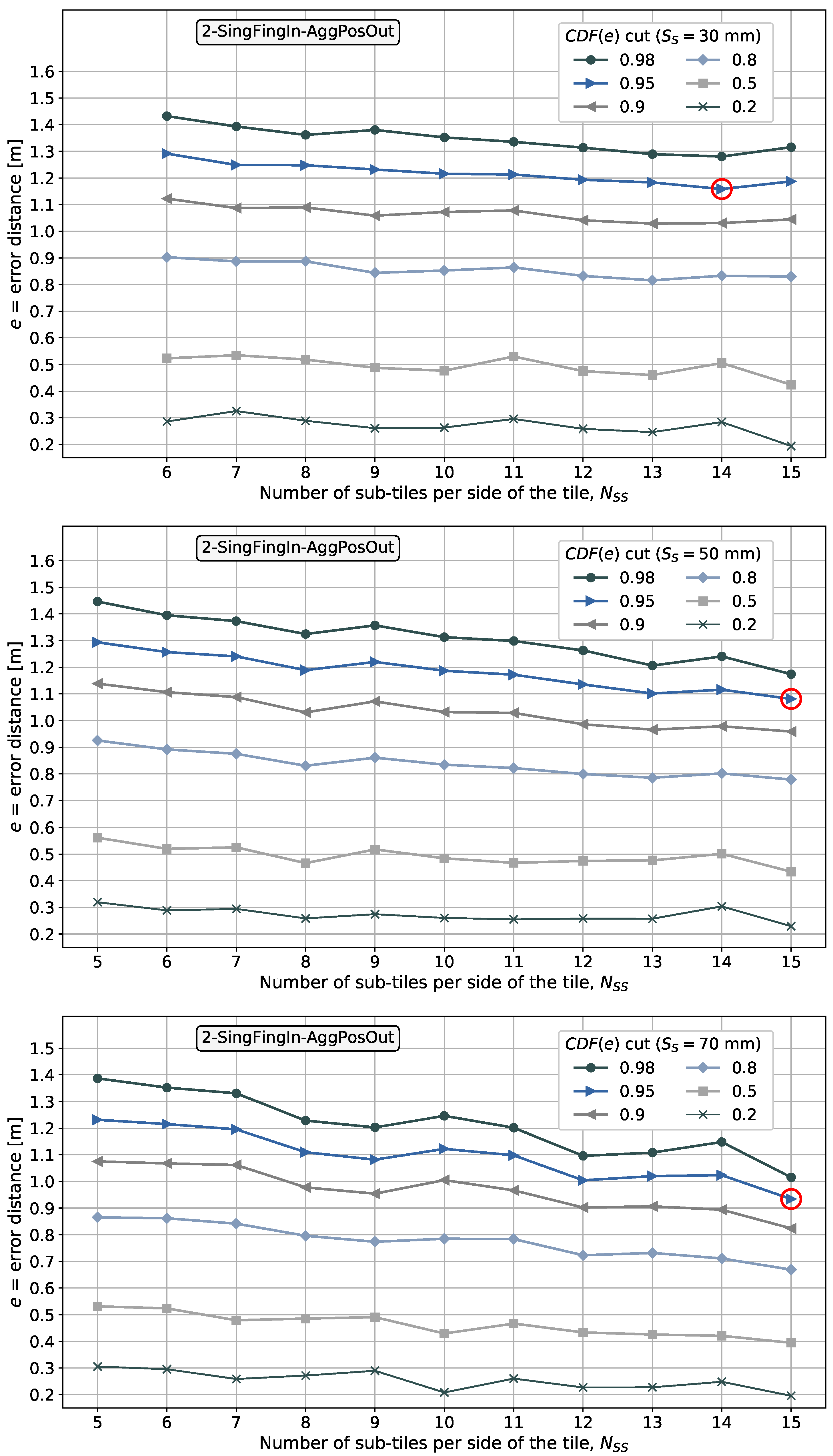
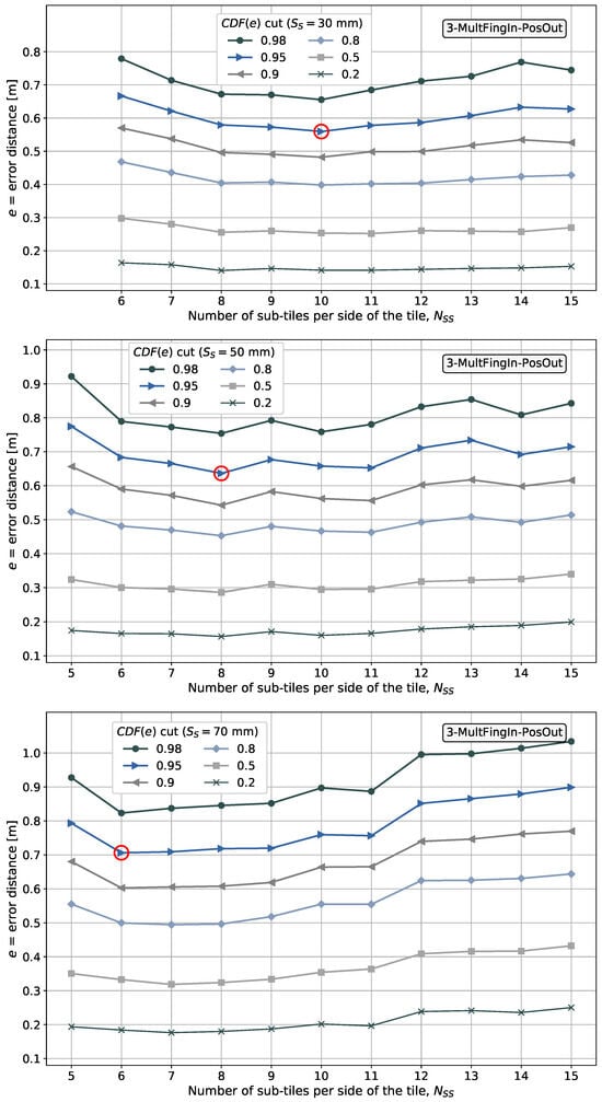
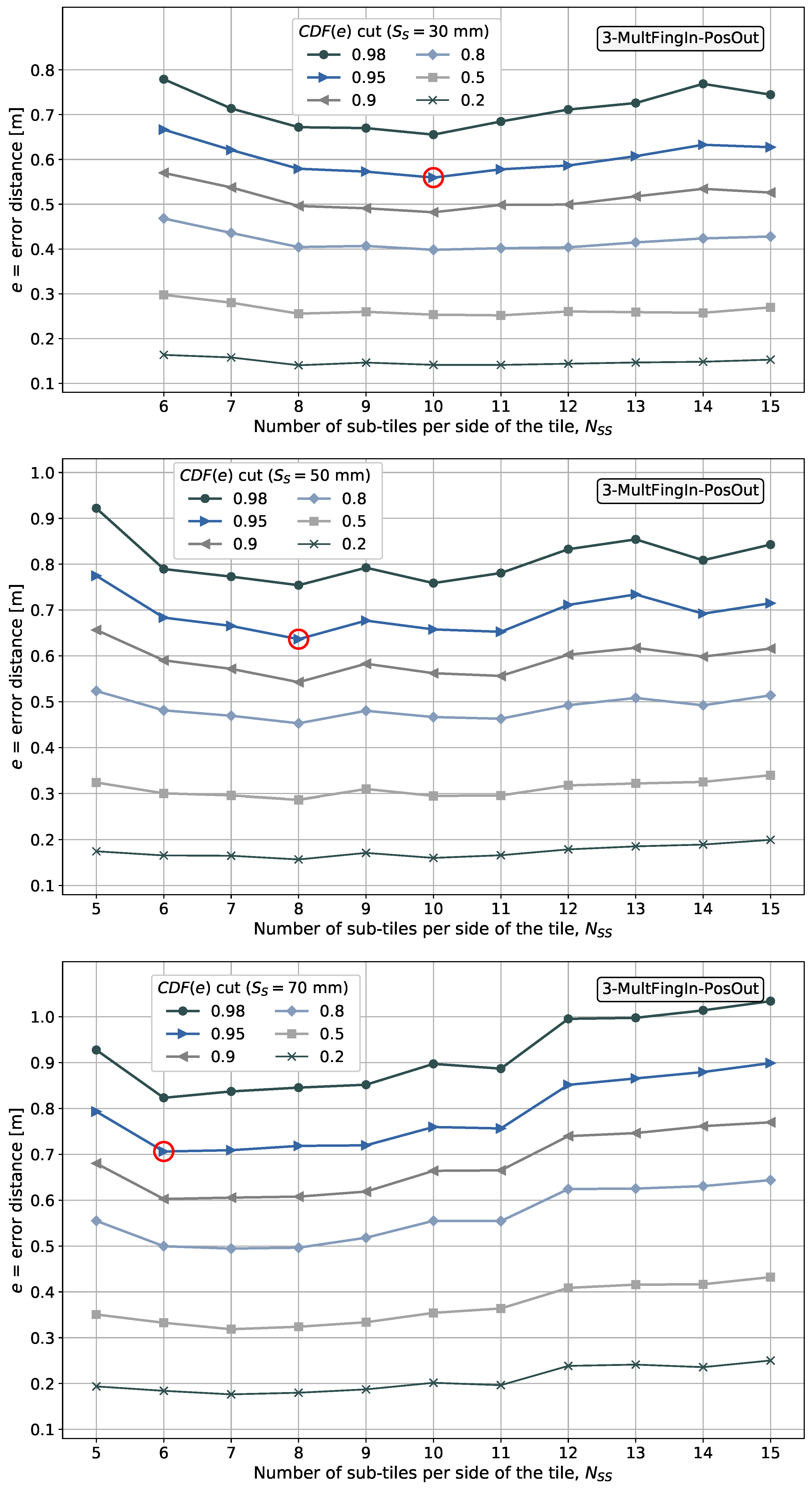
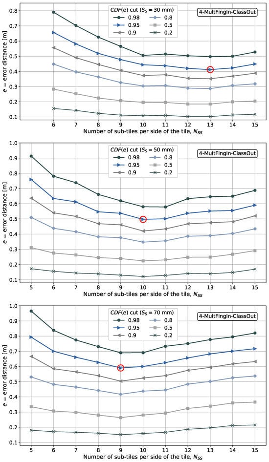
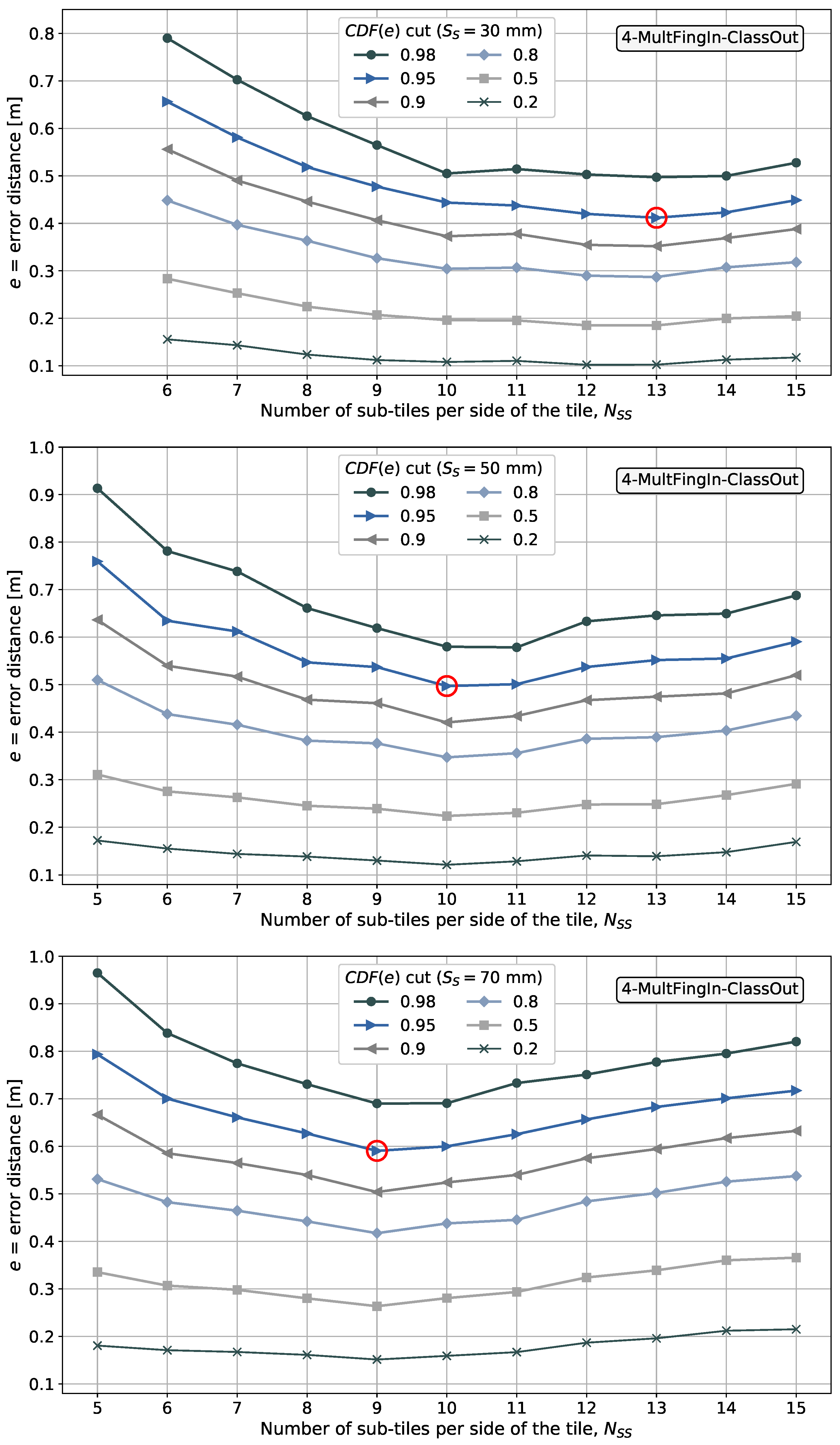
Figure 17.
Error distances from the cuts in the CDF of the error distances at different percentiles for the pattern-matching method 1-SingFingIn-PosOut for different numbers of sub-tiles per side of the tile and the three side lengths of the sub-tiles considered.
Figure 17.
Error distances from the cuts in the CDF of the error distances at different percentiles for the pattern-matching method 1-SingFingIn-PosOut for different numbers of sub-tiles per side of the tile and the three side lengths of the sub-tiles considered.
Figure 18.
Error distances from the cuts in the CDF of the error distances at different percentiles for the pattern-matching method 2-SingFingIn-AggPosOut for different numbers of sub-tiles per side of the tile and the three side lengths of the sub-tiles considered. The red circles indicate the minima at the 95th percentile for the interval of considered.
Figure 19.
Error distances from the cuts in the CDF of the error distances at different percentiles for the pattern-matching method 3-MultFingIn-PosOut for different numbers of sub-tiles per side of the tile and the three side lengths of the sub-tiles considered. The red circles indicate the minima at the 95th percentile for the interval of considered.
Figure 20.
Error distances from the cuts in the CDF of the error distances at different percentiles for the pattern-matching method 4-MultFingIn-ClassOut for different numbers of sub-tiles per side of the tile and the three side lengths of the sub-tiles considered. The red circles indicate the minima at the 95th percentile for the interval of considered.
Comparing the minima at the 95th percentile, as listed above, we observe that the smaller the tile (and 2D sensor array), the smaller the error distance given that for mm, the side length of the tile (2D sensor array) is mm mm, and for mm, the side length of the tile (2D sensor array) is mm mm.
As a summary of this method, we learn that there is an optimal size of the tile (and hence the 2D sensor array) that minimizes the error distance.
6.6. Comparison of the Results Among the Pattern-Matching Methods
From the results presented above for all of the pattern-matching methods, we select and compare the results for two specific distinctive cases, namely the following:
- Comparison of the results obtained with the smallest 2D sensor array considered for different side lengths of the sub-tiles among the different pattern-matching methods;
- Comparison of the best results obtained that minimize the error distance for different side lengths of the sub-tiles among the different pattern-matching methods.
These comparisons are carried out for the three side lengths of the sub-tiles, , that form part of the tile arrangements considered (Table 14).
6.6.1. Comparison of the Results Obtained Using the Smallest 2D Sensor Array Considered
From the results for all of the pattern-matching methods, we select the ones resulting from the smallest 2D sensor array considered for the three side lengths of the sub-tiles considered, namely the following:
- mm with ;
- mm with ;
- mm with .
Next, we compare how the different pattern-matching methods perform against one another in these cases in terms of minimizing the error distance. This comparison is presented in Figure 21. The results present the same pattern for the three side lengths of the sub-tiles considered. The methods 3-MultFingIn-PosOut and 4-MultFingIn-ClassOut perform better than the other methods. The method 4-MultFingIn-ClassOut performs slightly better than the method 3-MultFingIn-PosOut, although the difference may be negligible for practical considerations. The method 2-SingFingIn-AggPosOut performs better than 1-SingFingIn-PosOut but worse than 3-MultFingIn-PosOut and 4-MultFingIn-ClassOut.
The results found for each sub-tile size and pattern-matching method for the case of the smallest 2D sensor array are summarized in Table 15. The table lists the number of NN parameters for each combination of and and pattern-matching method.
Table 15.
Results for the smallest 2D sensor array for each side length of the sub-tiles and pattern-matching method.
The first and most important observation is that all of the methods that include spatial side information perform much better than the method that does not use side information, 1SingFingInPosOut. The second observation is that by relying on a more expensive NN model, in terms of the number of NN parameters, a better performance result can be obtained for the same input data. A third observation is that aggregating the results in the fingerprint domain (with the methods 3-MultFingIn-PosOut and 4-MultFingIn-ClassOut) produces better results than aggregating the position results in the position domain (with the method 2SingFingInAggPosOut).
As discussed above, we observe in Figure 21 that the methods 3-MultFingIn-PosOut and 4-MultFingIn-ClassOut perform almost the same in terms of the practical considerations. Assuming an equal distribution of the error distances for both methods, we can conclude that pattern-matching method 3-MultFingIn-PosOut is less expensive to implement than the method 4-MultFingIn-ClassOut in terms of the number of parameters required by the respective NN models. That is, the method 4-MultFingIn-ClassOut requires about to times more parameters than the method 3-MultFingIn-PosOut to produce presumably equal results. Thus, when adopting spatial side information, if the performance of the smallest sensor array is suitable for a given use-case, pattern-matching method 3-MultFingIn-PosOut would be the choice when aiming for a lighter method in terms of the computing resources.
It is noted that the column in Table 15 indicating the number of NN parameters for the method 2-SingFingIn-AggPosOut includes the number of instances of, or calls to, the NN model implemented in this method. The NN model is executed for each one of the sub-tiles in the tile. This is provided to indicate that for this method, the number of NN parameters alone is not representative of the computing cost of this method.
6.6.2. Comparison of the Best Results Obtained That Minimize the Error Distance
From the results for all of the pattern-matching methods, we select the best ones that minimize the error distance for the three side lengths of the sub-tiles considered. The best results found for each sub-tile size and pattern-matching method are summarized in Table 16. The table lists the number of NN parameters for each combination of and and pattern-matching method. Next, we compare how the different pattern-matching methods perform one against the other for these cases. This comparison is presented in Figure 22. The results present the same pattern for the three side lengths of the sub-tiles considered. The method 4-MultFingIn-ClassOut performs better than the other methods. This is followed, in decreasing order of error, by the method 3-MultFingIn-PosOut, the method 2-SingFingIn-AggPosOut, and finally by the method 1SingFingInPosOut.
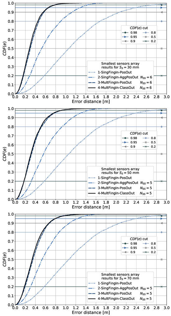
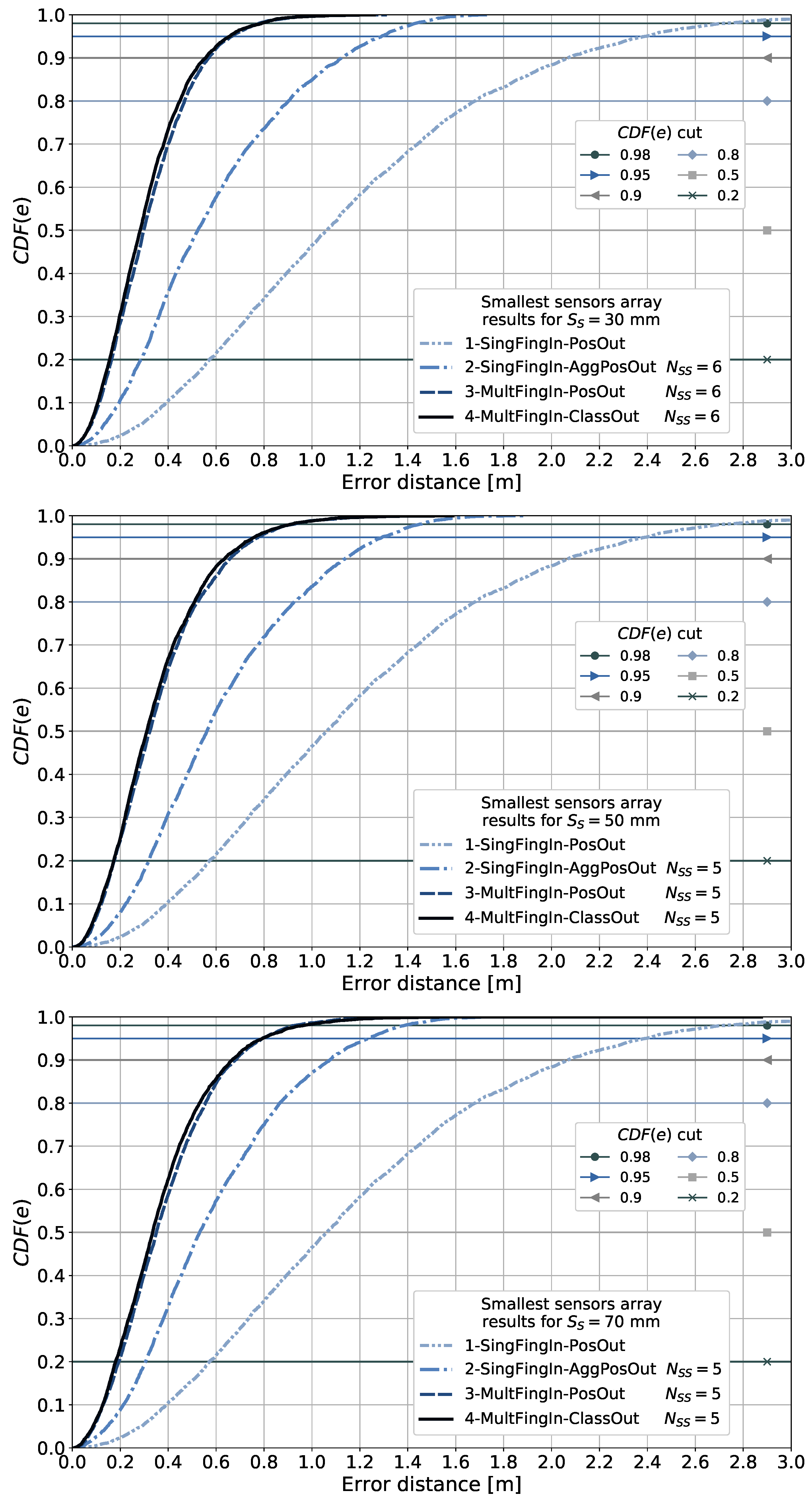
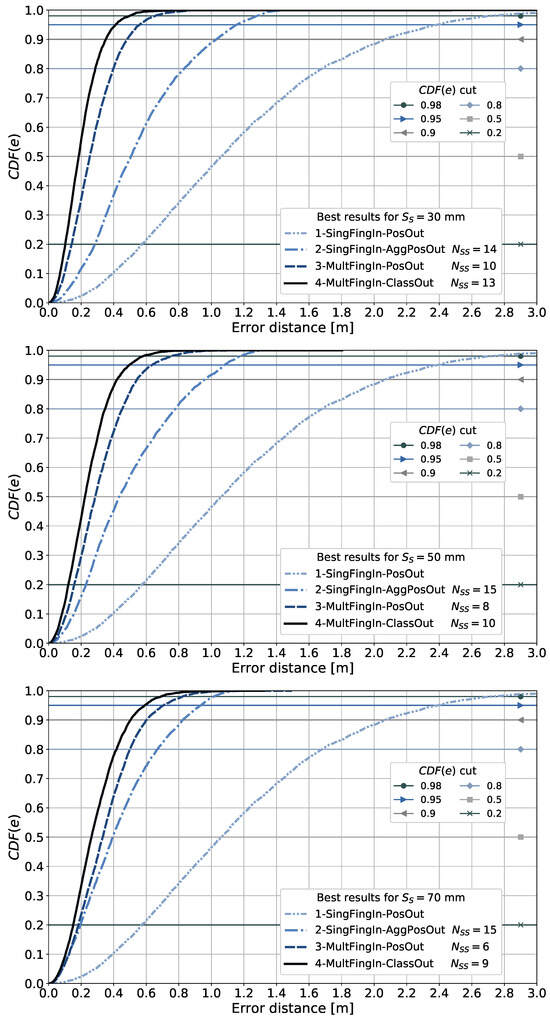
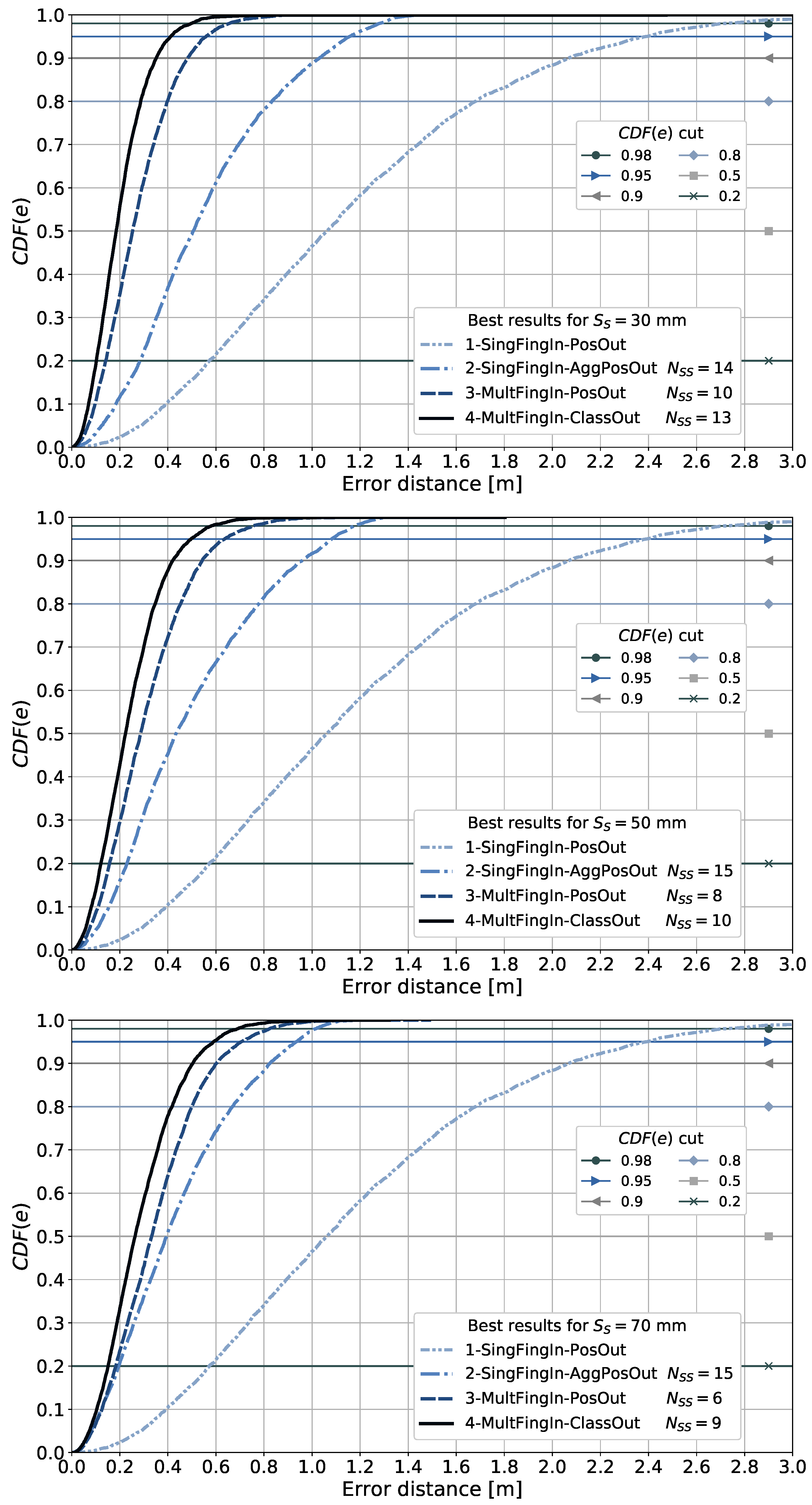
Figure 21.
Comparison of the results obtained using the smallest 2D sensor array considered among different pattern-matching methods for the three side lengths of the sub-tiles, , considered.
Figure 21.
Comparison of the results obtained using the smallest 2D sensor array considered among different pattern-matching methods for the three side lengths of the sub-tiles, , considered.
Figure 22.
Comparison of the best results obtained that minimize the error distance among different pattern-matching methods for the three side lengths of the sub-tiles, , considered.
Figure 22.
Comparison of the best results obtained that minimize the error distance among different pattern-matching methods for the three side lengths of the sub-tiles, , considered.
Table 16.
Best results for each side length of the sub-tiles and pattern-matching method.
Similar to the case for the smallest 2D sensor array, the first and most important observation is that all of the methods that include spatial side information perform much better than the method that does not use side information, 1-SingFingIn-PosOut. The second observation is that by relying on a more expensive NN model, in terms of the number of NN parameters, a better performance result can be obtained for the same input data. A third observation is that aggregating the results in the fingerprint domain (with the methods 3-MultFingIn-PosOut and 4-MultFingIn-ClassOut) produces better results than aggregating the position results in the position domain (with the method 2-SingFingIn-AggPosOut).
We observe in Figure 22 that pattern-matching method 4-MultFingIn-ClassOut has about 100 to 150 mm less error than the method 3-MultFingIn-PosOut at the 95th percentile in the CDF of the error distances. However, looking at Table 16, the method 4-MultFingIn-ClassOut requires about to times more parameters than the method 3-MultFingIn-PosOut does. Thus, it should be evaluated whether for a specific use-case the gain produced using the method 4-MultFingIn-ClassOut is worth the cost in terms of the number of NN parameters required and the associated computing costs.
It is noted that the column in Table 16 indicating the number of NN parameters for the method 2-SingFingIn-AggPosOut includes the number of instances of, or calls to, the NN model implemented in this method. The NN model is executed for each one of the sub-tiles in the tile. This is provided to indicate that for this method, the number of NN parameters alone is not representative of the computing cost of this method.
6.7. Pattern-Matching Method 4-MultFingIn-ClassOut Details
We study in detail the results obtained using pattern-matching method 4-MultFingIn-ClassOut since this is the method that produces the best result in terms of minimizing the error distance when compared with those of the other methods.
A selection of CDF curves of the error distances for different numbers of sub-tiles and sub-tile sizes is presented in Figure 23, Figure 24 and Figure 25. These figures depict the actual CDF curves from which we took the cuts at different percentiles depicted in Figure 20. Each CDF curve in Figure 23, Figure 24 and Figure 25 contains more information about the results for all of the percentiles than that presented in Figure 20; however, some curves were removed for legibility.
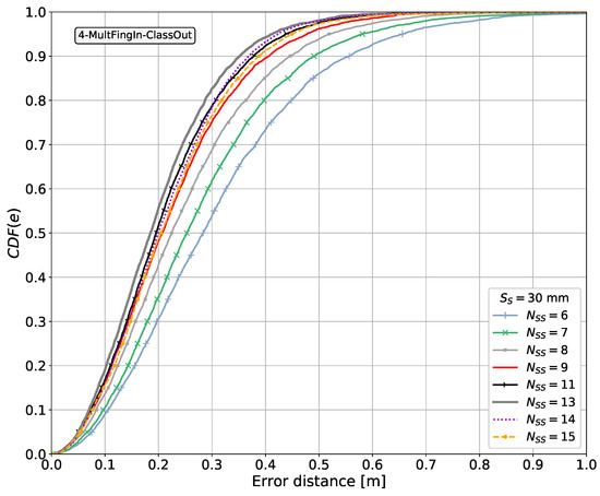
Figure 23.
Comparison of the results for the pattern-matching method 4-MultFingIn-ClassOut with a side length of the sub-tiles mm and different numbers of sub-tiles per side of the tile, .
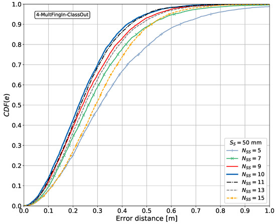
Figure 24.
Comparison of the results for the pattern-matching method 4-MultFingIn-ClassOut with a side length of the sub-tiles mm and different numbers of sub-tiles per side of the tile, .
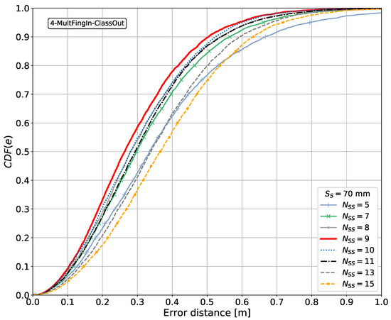
Figure 25.
Comparison of the results for the pattern-matching method 4-MultFingIn-ClassOut with a side length of the sub-tiles mm and different numbers of sub-tiles per side of the tile, .
In the CDF curves shown in Figure 23, Figure 24 and Figure 25, the curves depicted with continuous lines correspond to low values. More specifically, curves with continuous lines correspond to values ranging from the smallest number of sub-tiles considered to the that minimizes the error distance (regarded as the best ). The CDF curve for the best sets an upper bound on the performance, meaning that the results for any other will perform worse than those obtained for the best . This upper bound is depicted as a thicker continuous line. The curves for results with a number of sub-tiles, , greater than the best show a worse performance than this upper bound. These curves are observed on the right side of the curve for the best . These curves are represented using dashed lines, for legibility, to distinguish them from the curves representing the results for a lower (which are plotted using continuous lines). From these results, we can observe that it is meaningless to increase the number of sub-tiles to a greater number than the best since the performance starts to degrade. Therefore, the use of values greater than the best , that is, corresponding to the curves represented with dashed lines, is not a good option in the context of our study. This is because to obtain the performance represented by the dashed lines, a bigger 2D sensor array is required, plus the associated computing resources, for a performance that could be attained using a smaller 2D sensor array.
From the curves, we can also study the difference in the error at different percentiles to decide whether increasing the complexity and computing cost using a bigger 2D sensor array, that is, with more sub-tiles, is worth the reduction in the positioning error.
It is noted that pattern-matching method 3-MultFingIn-PosOut shows similar results to those of the method 4-MultFingIn-ClassOut, with the difference being that the former performs worse than the latter. Then, similar conclusions to those discussed above can be drawn for the pattern-matching method 3-MultFingIn-PosOut based on the results presented in Figure 19.
Finally, Figure 26 gathers the CDF curves for the best results (continuous lines) and for the results using the smallest 2D sensor array (dashed lines) for each side length of the sub-tiles using the method 4-MultFingIn-ClassOut. In this figure, we can observe the differences in the error distance when changing the side length of the sub-tiles, , for these distinctive cases.
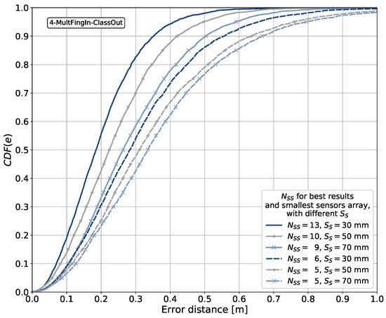
Figure 26.
Comparison of the best results (continuous lines) and the results with the smallest 2D sensor array (dashed lines) for the pattern-matching method 4-MultFingIn-ClassOut with different side lengths of the sub-tiles .
Although the smallest considered was selected by us, let us consider that the results for the smallest considered define a lower bound on the performance for the method 4-MultFingIn-ClassOut in the sense that this is the worst performance with the smallest number of NN parameters. Then, the dashed lines in Figure 26 represent the lower bound on the performance. The continuous lines in the figure, on the other hand, are the results for the best , meaning that these define the upper bound on the performance. Then, any number of sub-tiles per side of the tile between the minimum considered and the best found will lie between these bounds. It follows that for a given side length size of the sub-tiles, , the former conclusion can be interpreted as follows. The closest solution (as is a discrete parameter given by a natural number) in the number of sub-tiles per side of the tile, , with the minimum number of sub-tiles (and hence the minimum number of NN parameters) when aiming at a given operational point as a target will lie between these bounds. An operational point is defined in this context as a target error distance at a given percentile in the CDF of the error distances. Finally, the to be selected is that which satisfies a desired trade-off point between the cost and performance, along with other considerations—for example, the practical use of a given size of 2D sensor array.
We proposed above that the smallest considered can define a lower bound on the performance for the method 4-MultFingIn-ClassOut. Observe in Figure 20 that the error distance for with mm and with mm and mm, at the 95th percentile, is greater than the error distance for larger values of , at least in the interval of the number of sub-tiles from the smallest to the for the best results. The cases for the smallest sensor array are listed in Table 14 as the tile arrangements 6×6-30, 5×5-50, and 5×5-70. The corresponding number of NN parameters for these tile arrangements is listed in Table 14, and for convenience it is summarized in Table 15.
6.8. Observations for Cases with Spatial Side Information and Aggregation in the Fingerprint Domain
Below, we summarize different observations for cases using spatial side information and aggregation of the fingerprints in the fingerprint domain, namely pattern-matching methods 3-MultFingIn-PosOut and 4-MultFingIn-ClassOut.
6.8.1. Lower Bound in Performance for the Smallest 2D Sensor Array Considered
From the results obtained using pattern-matching methods 3-MultFingIn-PosOut and 4-MultFingIn-ClassOut, we observe in Figure 19 and Figure 20 the following trend. This trend indicates that on starting with a small number of sub-tiles and then increasing the amount of side information by adding more sub-tiles, that is, increasing , the error distance decreases until the that produces the best result with the minimum error distance (the best ). Then, the results when selecting a small 2D sensor array can be used to define a lower bound in the performance. Here, because the number of NN parameters grows with , the lower bound in performance exists in the context of obtaining the worst error distance using the smallest number of NN parameters. This means that selecting a bigger 2D sensor array will result in a smaller positioning error up to the that produces the best result. So, the smallest 2D sensor array considered is regarded to be that producing the worst result with the smallest number of sub-tiles, , that can be obtained using these methods.
For the smallest 2D sensor arrays considered, we selected equivalent tile sizes consisting of the following numbers of sub-tiles: , with mm, and , with mm and mm. This selection was based on practical observations. The first observation is the quadratic growth in the number of tiles required to cover the whole positioning area, as a function of the inverse of the side length of the tiles. The smaller the tiles, the greater the number of tiles required to cover the positioning area, and the greater the number of reference positions associated with the fingerprint samples that needs to be collected. Thus, operating using a large number of small tiles to cover the positioning area adds overheads in terms of the time and costs required to collect the fingerprint samples in a real scenario. Another aspect to consider is that the greater the number of tiles, the greater the number of tile-classes required in pattern-matching method 4-MultFingIn-ClassOut. This translates to selecting an NN with a suitable representational capacity for the number of output classes. The second observation is related to pattern-matching method 4-MultFingIn-ClassOut and the convolution operation. In general, there is a requirement for the minimum size of the tensor input to a CNN such that it is suitable for actually performing the convolution operation. In method four, the tensor input to the CNN is a tensor of fingerprints. Then, the number of sub-tiles in a tile must be greater than the convolution kernel combined with the stride size. In pattern-matching method 4-MultFingIn-ClassOut, we used a convolution kernel of and a stride size of 1; therefore, we adopted a minimum number of sub-tiles per side of the tile of .
Now, it is noted that the worst error distance with the smallest number of NN parameters considered (the smallest considered, with and 6) reduced the positioning error in distances ranging from to m, for the three considered, to that in the case without spatial side information using pattern-matching method 1-SingFingIn-PosOut, measured at the 95th percentile in Figure 21. This is equivalent to an order of to of the side lengths of the 2D sensor array. This last observation is an attempt to normalize in the 2D sensor array sizes the gain obtained using the different 2D sensor array sizes, under the assumption that the size of the 2D sensor array defines the positioning resolution for the samples.
As a summary of the results obtained using the smallest 2D sensor array, we observe that the reduction in the error distance is significant when compared with fingerprintingbased positioning implementing pointwise samples and no side information (patternmatching method 1-SingFingIn-PosOut). For a given use-case, it should be evaluated whether the use of a small 2D sensor array suffices in terms of the desired trade-offs between the cost, complexity, and intended target error distance at a given percentile in the CDF of the error distances (or, alternatively, target distribution of the error distances).
6.8.2. Two-Dimensional Sensor Array Sizes and Positioning Errors for the Best Results
Table 17 lists the error distances at the 95th percentile in the CDF of the error distances for the best results obtained using pattern-matching methods 3-MultFingIn-PosOut and 4-MultFingIn-ClassOut (Figure 22 and Figure 26) for the three side lengths of the sub-tiles considered. This table complements Table 16, which details the number of NN parameters, the best obtained, and the side length of the tile for each considered.
Table 17.
Error distances at the 95th percentile in the CDF of the error distances for the best results obtained using pattern-matching methods 3-MultFingIn-PosOut and 4-MultFingIn-ClassOut (Figure 22 and Figure 26), normalization of the error distances at the 95th percentile to the side length of the tiles (2D sensor array), and the difference in the error distances between these methods and the method 1-SingFingIn-PosOut. Results for the three side lengths of the sub-tiles considered.
As was mentioned before, we observe in Table 17 that the error distances at the 95th percentile decrease with the sub-tile sizes given by . The tile size, which is the size of the 2D sensor array, is correlated with this observation. That is, the smaller , the smaller the error distance and the size of the 2D sensor array, given by . So, from the results obtained, when decreases, increases, but overall, the 2D sensor array size given by the side length of the tile, , decreases. When the tile size decreases, there are more tiles in the positioning area, with smaller inter-tile distances, which seems to contribute to a finer granularity for estimating the position.
To complement the explanation above, it is noted that the size of the 2D sensor array in each case is calculated from the side length of the tile, , which is a function of and the best obtained for each case. The side lengths of the tiles for each case are listed in Table 16. It follows from the results obtained that decreases with the sub-tile size given by .
In Section 6.4 and Section 6.5, it was hypothesized that the bigger the tile, the coarser the resolution for estimating the position due to the increased inter-tile distance. A trade-off between increasing the amount of side information through increasing and the effects of increasing the inter-tile distance for a given fixed side length of the sub-tile was also hypothesized.
As it is observed that a reduction in the error distance is correlated with small side lengths of the sub-tiles and a large number of sub-tiles but at the same time correlated with small tile sizes, a new hypothesis can be formulated. The new hypothesis can be stated as follows. For the given assumptions, the sub-tile should decrease in size through the parameter and the number of sub-tiles in the tile should increase through the parameter such that the combination of parameters and is constrained to result in a side length of the tile that is small enough to produce a finer granularity or resolution for estimating the position.
Actually, regarding the size of the 2D sensor array, we may expect a constraint to counteract how small the 2D sensor array can be from the actual physical arrangement of the antennas or receivers in the sensors array (as discussed in Section 7.2). However, such a constraint is not part of our assumptions.
From an ideal assumption in which the 2D sensor array size or tile size can define the positioning granularity or resolution, we proceed as follows. We normalize the error distances obtained for each pattern-matching method and side length of the sub-tiles by the corresponding side length of the 2D sensor array. In Table 17, we observe that for the case of pattern-matching method 3-MultFingIn-PosOut, the error distance normalized by the 2D sensor array’s size is between and times the side length of the 2D sensor array. For the method 4-MultFingIn-ClassOut, the normalized error distance is approximately in the order of the side length of the 2D sensor array ( to times the side length of the 2D sensor array). Under the ideal assumptions, the latter observation means that at least 95 percent of the measurements have an error distance equal to or below the sampling resolution used by the 2D sensor array (where the sampling resolution is equivalent to the tile sizes used to sample the whole positioning area).
Table 17 also lists the differences between the error distance obtained using the pattern-matching method without side information, 1-SingFingIn-PosOut, and the error distances obtained using the methods 3-MultFingIn-PosOut and 4-MultFingIn-ClassOut, measured at the 95th percentile of the CDFs of the error distance. In addition, we listed the difference in the error distance observed between the methods 3-MultFingIn-PosOut and 4-MultFingIn-ClassOut measured at the 95th percentile of the CDFs of the error distance.
- ○
- Discussion About the Reduction in the Size of the 2D Sensor Array and ConstraintsThe observation mentioned above, discussing that at least 95 percent of the measurements have an error distance equal to or below the sampling resolution used by the 2D sensor array opens many research questions. For example, one line of thought suggests that the smaller the 2D sensor array, the smaller the positioning error. The reduction in the size of the 2D sensor array or tile is actually controlled by the combined result of reducing the side lengths of the sub-tiles, , and increasing the number of sub-tiles per side of the tile, . Thus, if this trend continues, near the limit, we would have a very small 2D sensor array with a large number of sensors. Decreasing the 2D sensor array further to the limit so that it converges to what is ideally a point on a 2D positioning plane, it can be thought that the minimization of the positioning error is not due to the availability of adjacent samples but due to the high number of samples collected at that point. However, note that this observation is associated with the assumed collection of training samples from every position delimited by fixed tiles, which in this case would be assumed for every single point on the positioning plane (and which at the limit will be an infinite number of points). Then, this view challenges the idea of benefiting from using spatial side information, suggesting that taking a high number of samples at a single point would produce better results than collecting samples at adjacent points. Yet this generates many questions. The instantaneous and simultaneous collection of samples using multiple sensors or receivers is not physically possible when all of the sensors converge to a single point. Then, we can think about using a single sensor or receiver and taking a high number of samples in the time domain, as has been suggested in some research works in the past. However, the initial observation was based on the assumption of the sampling of the entire positioning area. The sampling of the entire positioning area is realistically feasible if it is performed using a 2D sensor array with a size equivalent to a tile size of, say, above mm2. The sampling can be achieved using a certain mechanized process. One example could be sampling fingerprints using a robot driven by stepping motors. Another example could be using for the sampling the same machinery that needs the positioning information, taking overlapped samples, which will then be post-processed as training tiles. In contrast, it is not realistic to sample every point in the positioning area when the meaning of a point is defined in a mathematical sense, or even when it is defined as a very small discretized area. Another observation is that if there are no adjacent samples, it is not possible to perform the convolution operation in pattern-matching method 4-MultFingIn-ClassOut.Another line of thought is that in our assumptions, we did not consider the actual antenna design aspects related to the construction of the 2D sensor array, such as the effects and constraints of the inter-antenna spacing. These may counteract the performance gain experienced when reducing the 2D sensor array’s size in a real system. It was observed that for the system under consideration, there is a correlation between the reduction in the 2D sensor array’s size and the reduction in the positioning error. However, in reality, it could be expected that the physical arrangement of the sensors will introduce constraints that will counteract this trend. For example, in the case of implementing the 2D sensor array with an array of antennas, the inter-antenna spacing will add a constraint. In the case of implementing the 2D sensor array with a mechanical device sampling all of the positions equivalent to the sub-tiles, the precision of the mechanism and possible vibrations in the sequential sampling will add a constraint limiting the smallest possible size of the 2D sensor array. This consideration is discussed in Section 7.2.Yet, another line of thought is based on the idea that it would be beneficial to exploit the side information from adjacent positions as far as possible from the target position. This is based on the idea that the further apart the sensors are, the more the RSS level may vary enough to counteract the variations due to the fading. A possible research direction associated with this line of thought would be to study the use of side information collected using a kind of 2D sensor array with sparse sensors.
6.8.3. The Best Results and Border Conditions in the Positioning Area in the Scenario
We discussed in Section 5.3 the border conditions in the area intended for positioning in the scenario. In the training phase, the whole positioning area will be covered with entire tiles that are contiguous to each other (fixed tiles); that is, the use of fractions of a tile (and the 2D sensor array) is not considered in our scope. Then, for cases with tile arrangements in which the dimensions of the area intended for positioning are not a multiple of the side length of the tile, some regions of the area intended for positioning will be uncovered, at the top or right borders or at both.
Furthermore, we discussed in Section 5.10 that the size of the 2D sensor array limits the useful area in which the positioning can be performed. Considering the center of the 2D sensor array as the reference for determining the position, bigger 2D sensor arrays cannot come as close to the borders to perform positioning as smaller ones can. Thus, the useful area in which the positioning can be performed changes with the size of the 2D sensor array (and tile arrangement). Or, in other words, the uncovered areas adjacent to the borders appear as stripes with a width (assuming the center of the 2D sensor array as the reference for determining the position).
Now, we would like to study whether the fact that some tile arrangements do not fill the entire area intended for positioning and the fact that different tile arrangements produce more or less samples close to the borders of the positioning area cause any change in the results obtained using pattern-matching methods 3-MultFingIn-PosOut and 4-MultFingIn-ClassOut. So, in other words, we would like to know whether the CDF curves of the error distances shift due to a varying number of samples with different statistics close to the borders as a result of using different tile arrangements. The CDFs of the error distances obtained using these methods for the best results were discussed in Section 6.6.2 and are shown in Figure 22. For the particular case of the method 4-MultFingIn-ClassOut, the results were discussed in Section 6.7 and are shown in Figure 26. For convenience and simplicity, we will use as a reference the pattern-matching method 4-MultFingIn-ClassOut. Similar conclusions can be drawn for the method 3-MultFingIn-PosOut.
First, we observe that the best result that minimizes the CDF of the error distances with mm and the method 4-MultFingIn-ClassOut is obtained with . This results in a tile with a side length of mm. For this tile arrangement, the maximum allowed dimensions of the area intended for positioning (13,000 mm × 5000 mm) are a multiple of , meaning that the area intended for positioning will be covered entirely by fixed tiles in the tiling process (through the execution of the function , listed in Pseudocode 1). Thus, for this tile arrangement, the positioning area is equivalent to the area intended for positioning; that is, there are no uncovered regions next to the borders. Hence, the results obtained for this tile arrangement cannot be affected by missing samples at the borders due to the impossibility of covering the entire area intended for positioning. Then, for this case (a tile arrangement with mm and ), the CDF curve depicted in Figure 26 can be considered a trusted reference; that is, it is not shifted by the effect of tiles not fitting into the scenario.
Next, we aim to determine whether there is a characteristic pattern of the error distances when samples from the MTT dataset are observed in the positioning area. In this context, a characteristic pattern would be, for example, some kind of concentration of the error distances into some parts of the 2D positioning area. In particular, we will observe the pattern for the error distances in samples next to the borders. If, for example, there is a pattern in the error distances in which there is a concentration of a particular range of error distances close to the borders, the effect of the untiled stripes adjacent to the borders could lead to a change in the distribution of the error distances. In this case, a shift in the error distance CDFs would be a consequence of the different patterns of error distances contributing to the final distribution for a given tile arrangement and the resulting positioning area.
We proceed to make an initial observation of the error distances in the positioning area. We use as reference the tile arrangement with mm and , which is the best result obtained using pattern-matching method 4-MultFingIn-ClassOut for mm. Figure 27 shows with crosses the center positions of the moving tiles from the MTT dataset for this tile arrangement at the corresponding ground truth reference positions in the 2D positioning area in the scenario. The color of the crosses indicates the error distance according to the scale shown in the figure. In this figure, we do not observe any characteristic pattern that could lead to changes in the results. There is no characteristic concentration of the error distances close to the borders. Certainly, we can spot some clusters where certain ranges of error distances are concentrated in different parts of the positioning area; however, this is attributed to the radio channel realizations and a lack of enough samples. It should be noted that due to the symmetry of the scenario, the same statistics should be observed in the four quadrants of the positioning area. This observation is based on the symmetry of the scenario along the two coordinates. In this case, the density of the samples can be quadrupled in one-quarter of the scenario to obtain a more complete appreciation of the statistics of the results. Given the symmetry of the scenario, we can imagine dividing the scenario into four parts (in two halves, along each dimension) and then merging these four parts (mirroring along the vertical and/or horizontal axis accordingly) to increase the density of the samples.
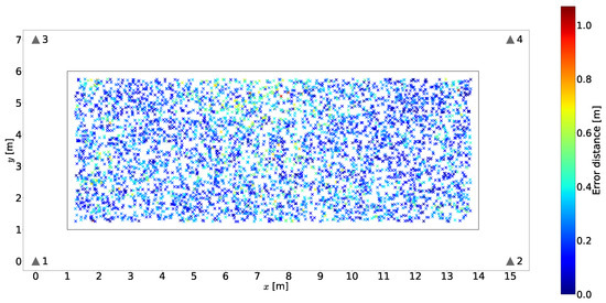
Figure 27.
Positioning area in the selected scenario showing the center positions of the moving tiles from the MTT dataset, represented by crosses. The best result with pattern-matching method 4MultFingInClassOut for the tile arrangement with and mm. The color of the crosses indicates the error distance according to the scale shown on the right side of the figure.
Observing the other tile arrangements, we reached the same conclusions as those discussed above. For example, Figure 28 shows with crosses the center positions of the moving tiles from the MTT dataset at the corresponding ground truth reference positions in the positioning area in the scenario for a tile arrangement with mm and . In this figure, we do not observe any characteristic pattern that could lead to changes in the results.
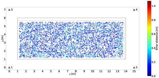
Figure 28.
Positioning area in the selected scenario showing the center positions of the moving tiles from the MTT dataset, represented by crosses. The best result with pattern-matching method 4MultFingInClassOut for the tile arrangement with and mm. The color of the crosses indicates the error distance according to the scale shown on the right side of the figure. The empty stripes on the top and right sides of the positioning area are due to the tiling process using entire tiles, leaving a region of the area intended for positioning uncovered, as explained in Section 5.3.
The observations above are based on a visual inspection of the samples. A formal study was carried out which consisted of removing a selection of samples from all of the samples covering the positioning area (the complete MTT dataset) to form a reduced dataset. This study was carried out for different tile arrangements. The samples removed were inside stripes of different widths, of up to 500 mm, adjacent to the inner borders of the area intended for positioning. Then, the error distance was calculated for the reduced dataset (without samples close to the borders). The CDF of the error distances corresponding to the reduced dataset was plotted and compared with the corresponding CDF considering all of the samples (the complete MTT dataset), such as the CDFs shown in Figure 26. We observed that the CDFs corresponding to the error distances from the reduced and complete datasets (the datasets without and with samples at the borders) almost overlapped, with negligible differences that could be attributed to the lack of enough samples. Thus, we conclude, as observed above, that removing samples next to the borders does not change the distribution of the error distances.
6.9. Notes on the Computing Costs for the Proposed Pattern-Matching Methods
Computing costs were not considered as a performance metric in the evaluation of the proposed pattern-matching methods, firstly because our primary goal was to obtain an initial assessment of the possible gains achievable using spatial side information, regardless of the computing costs, and secondly because the absolute computing costs alone are not regarded by us as a metric for selecting one pattern-matching method over another. We argue that what is important is the combined cost–performance of the entire positioning system, including the infrastructure, energy consumption, maintenance costs, etc. Therefore, the ultimate decision on adopting one pattern-matching method or another needs to be studied case by case.
Performance in terms of the training time was left out of our scope from the perspective that in practice, it depends on the following aspects. In the hardware domain, the training time depends on the CPU and GPU architecture, the associated memory, and the clock frequencies. In the software domain, it will depend on the programming language, actual implementation, and libraries used. Therefore, we find it more useful to report the training effort in terms of the number of NN parameters for each pattern-matching method and tile arrangement. These are listed in Table 14 and summarized for notable cases in Table 15 and Table 16.
6.10. Reproducibility of the Results
The training, validation, and testing datasets were synthetically generated, as is described in Section 5.2, using the system simulator presented in Section 5. Our results can be reproduced through the implementation of the system simulator along with the NN structures presented in the same section.
7. Summary, Conclusions, and Discussion
We presented the idea of exploiting spatial side information on fingerprints from adjacent positions relative to a target position with the purpose of minimizing the positioning error in fingerprinting-based positioning. We proposed increasing the complexity on the positioning device side by implementing a 2D sensor array that would allow us to collect physically adjacent RSS fingerprints. Our primary goal was to learn whether using spatial side information on RSS fingerprints, by means of an ideal 2D sensor array, could lead to a justifiable gain in terms of minimizing the positioning error.
To put our work into context, we provided a differentiation between fingerprinting in uplink and downlink cases, the possible uses of side information, and a classification of the possible positioning data aggregation domains. The literature related to the topic of our research was surveyed.
Then, we developed the concepts related to fingerprinting-based positioning with spatial side information in downlink and presented three pattern-matching methods for estimating the position by processing fingerprints with spatial side information. Two methods were based on regression, implemented with FFNNs, and one method was based on the classification of fractions of the positioning area, implemented with a CNN. In one method, positioning data aggregation was carried out in the position domain. In the other two methods, positioning data aggregation was carried out in the fingerprint domain.
The idea of exploiting spatial side information on fingerprints, along with the proposed pattern-matching methods, was benchmarked using a system simulator based on Monte Carlo methods. The simulator creates a scenario for positioning, generates synthetic fingerprints based on an indoor radio channel model, constructs arrangements of the fingerprints (tiles) that are equivalent to samples of the 2D sensor array, implements the pattern-matching methods, estimates the positions with each method, and calculates the positioning error for each one of the proposed methods. The cases without and with spatial side information were benchmarked.
7.1. Conclusions
From the results presented in the previous section, we draw the following conclusions. In our study, we proposed a system composed of a 2D sensor array, a given scenario, and the pattern-matching methods considered. It was observed that for the given assumptions and the system proposed, fingerprintingbased positioning with spatial side information substantially reduces the positioning error. The reduction in the positioning error is attained at the expense of implementing a 2D sensor array and additional computing hardware on the positioning device side.
7.1.1. Conclusions on the Use of Spatial Side Information
The performance of the proposed pattern-matching methods was measured in terms of the error distance, , given by Equation (1). From the results obtained using the four pattern-matching methods considered, as discussed in Section 6.6, we make the following observation. For cases using the smallest 2D sensor array and cases using the best number of sub-tiles that minimizes the error distance, all of the methods implementing spatial side information perform much better than the method that does not use side information, 1-SingFingIn-PosOut. This observation is summarized in the CDFs of the error distances shown in Figure 21 and Figure 22. In addition, the same observation can be made by comparing the results distributed in Section 6. Looking at the error distances for each one of the tile arrangements considered (combination of the parameters and ), shown in Figure 17, Figure 18, Figure 19 and Figure 20, it is observed that the pattern-matching methods that make use of spatial side information always perform better than the method that does not use spatial side information. From this observation it is concluded that for the system and assumptions considered, the use of spatial side information helps to minimize the positioning error.
7.1.2. Conclusions on the Aggregation of Fingerprints in the Fingerprint Domain
As an additional goal, we were interested in the exploitation of spatial side information in the fingerprint domain—that is, before the fingerprints were mapped to an estimated position using a pattern-matching method.
Pattern-matching methods 3-MultFingIn-PosOut and 4-MultFingIn-ClassOut make use of spatial side information in the fingerprint domain, aggregating fingerprints in this domain. These two pattern-matching methods perform better than pattern-matching method 2-SingFingIn-AggPosOut, which aggregates the estimated positions in the position domain, in terms of minimizing the positioning error. The results that summarize this observation are shown in Figure 21 and Figure 22.
7.2. Possible Limitations from the Assumptions
The actual description of how the 2D sensor array should be built is out of our scope. Each sensor, in charge of sampling the fingerprints for a sub-tile, could be constructed using an antenna or a receiver with a built-in antenna. Thus, it may be composed of an antenna array or a receiver array.
We did not consider the actual antenna design aspects related to the construction of the 2D sensor array. In this context, we worked with the numeric modules equivalent to the received signal strength, ignoring the effects of the constructive/destructive phases of radio-waves, the optimal antenna spacing, the effect on the antenna spacing and SNR, and variable AoAs of the radio-waves with respect to the 2D sensor array’s position.
It was observed that for the methods 3-MultFingIn-PosOut and 4-MultFingInClassOut, strictly for the given assumptions and system considered, the smaller the sub-tile size (and hence the smaller the 2D sensor array) the smaller the error distance (or, in other words, the better the performance in terms of minimizing the positioning error; see Section 6.4 and Section 6.5). These results are valid for the given assumptions and the system considered. However, it is counterintuitive to us that a smaller 2D sensor array leads to a better performance. It should be noted that we ignored some practical considerations present in a real system, as mentioned above, which may counteract the performance gain experienced when reducing the 2D sensor array’s size in a real system.
The side lengths of the 2D sensor array (tiles) at which the best results were found using pattern-matching methods 3-MultFingIn-PosOut and 4-MultFingIn-ClassOut are summarized in Table 16.
We observe in Table 16 that for the best results obtained with pattern-matching methods 3-MultFingIn-PosOut and 4-MultFingIn-ClassOut, when the sub-tile and tile sizes decrease, the number of sub-tiles in the tiles (2D sensor array) increases. So, one conjecture is the following. Since we do not have a constraint in terms of the actual antenna design aspects related to the construction of the 2D sensor array, the best solution aims to increase the number of fingerprint contributions from the side information while reducing the tile size. This could be the result of the system aiming to decrease the inter-tile distance to increase the positioning resolution while increasing the amount of side information.
7.3. Discussion
For the given assumptions and the system considered, we found through the system simulations that it is feasible to exploit spatial side information to minimize the positioning error. The gains observed in our simplified system, minimizing the error distance, pave the way for either studying fingerprinting-based positioning and spatial side information with a more elaborated system or validating whether the proposed 2D sensor array offers gains in a real system. In this latter case, the fingerprints would be collected from field measurements in a real scenario.
We postulated one conjecture based on the idea that by increasing the number of spatial points in which the fingerprints are measured, the amount of information should increase, and therefore, a better estimate of the position should be achieved. From the results obtained, such a conjecture is true for the system and assumptions considered.
We postulated another conjecture stating that a pattern-matching method based on the classification of discretized areas (the method 4-MultFingIn-ClassOut) could be applied to estimating the position. From the results obtained, such a conjecture is true for the system and assumptions considered, and in addition, it allows us to enhance the position estimate compared with that obtained using the other methods considered.
Looking at the computing and hardware costs alone, as an isolated unit, the proposed approach could appear to be expensive. In order to implement the proposed approach, it is necessary to incorporate the 2D sensor array on the positioning device side. In addition, it is necessary to incorporate on the positioning device side the necessary hardware to support the implementation of a pattern-matching method for processing the spatial side information. However, as stated in the introduction, we aim to transfer the complexity and cost from the infrastructure to the positioning device. Then, it is just a matter of taking a holistic view of the costs, complexity, energy efficiency, etc., in a given use-case to determine whether the implementation of the proposed approach fulfills the expected goals. These aspects are proper to each use-case and therefore cannot be generalized here. The ultimate feasibility in deciding whether to incorporate the proposed approach into a real use-case has to be analyzed on a case-by-case basis.
7.4. Directions for Future Work
Future work could address the following items:
- Studying the effects of positioning considering the rotation along the vertical axis and tilting on the horizontal axes of the 2D sensor array.
- Modeling of the 2D sensor array as, for example, an antenna array, considering the effects of constructive and destructive waves for a given antenna spacing, the AoA of the radio-waves, etc.
- A performance evaluation of a 2D sensor array using datasets obtained from field measurements.
- Exploration of alternative pattern-matching methods or an enhancement to the proposed methods.
- The use of other tile arrangements.
- The use of overlapping fixed tiles.
- The use of any other tile format or shape. For example, an interesting tile format to consider would be hexagonal-shaped tiles.
- The use of spatial side information collected using a kind of 2D sensor array with sparse sensors—for example, distributed along the machinery or object(s) performing the positioning.
- Alternative mappings from the tile-classes to the positions using pattern-matching method 4-MultFingIn-ClassOut.
Author Contributions
Conceptualization, S.L.; methodology, S.L.; software, S.L.; validation, S.L. and S.H.; formal analysis, S.L.; investigation, S.L.; resources, S.H., S.R., T.C., and P.K.; initial experimental dataset generation, S.H., L.T., and S.L.; hardware setup and support, S.R.; hybrid positioning system consulting, P.K.; writing, S.L.; review, S.L, S.H., and P.K.; visualization, S.L.; supervision, S.H. All authors have read and agreed to the published version of the manuscript.
Funding
This research received no external funding.
Data Availability Statement
The datasets used in this study were synthetically generated using the system simulator described in Section 5. A description of how to generate the datasets to reproduce the results is contained within the article in Section 5.2 (Generation of Datasets of Fingerprints). The datasets can be generated by implementing the first seven steps of the system simulator explained in Section 5.6.1.
Conflicts of Interest
All of the authors are employed by VTT Technical Research Centre of Finland Ltd.
References
- De Lima, C.; Belot, D.; Berkvens, R.; Bourdoux, A.; Dardari, D.; Guillaud, M.; Isomursu, M.; Lohan, E.S.; Miao, Y.; Barreto, A.N.; et al. Convergent Communication, Sensing and Localization in 6G Systems: An Overview of Technologies, Opportunities and Challenges. IEEE Access 2021, 9, 26902–26925. [Google Scholar] [CrossRef]
- Pin Tan, D.K.; He, J.; Li, Y.; Bayesteh, A.; Chen, Y.; Zhu, P.; Tong, W. Integrated Sensing and Communication in 6G: Motivations, Use Cases, Requirements, Challenges and Future Directions. In Proceedings of the 2021 1st IEEE International Online Symposium on Joint Communications and Sensing, Dresden, Germany, 23–24 February 2021; pp. 1–6. [Google Scholar] [CrossRef]
- Liu, F.; Cui, Y.; Masouros, C.; Xu, J.; Han, T.X.; Eldar, Y.C.; Buzzi, S. Integrated Sensing and Communications: Toward Dual-Functional Wireless Networks for 6G and Beyond. IEEE J. Sel. Areas Commun. 2022, 40, 1728–1767. [Google Scholar] [CrossRef]
- Chepuri, S.P.; Shlezinger, N.; Liu, F.; Alexandropoulos, G.C.; Buzzi, S.; Eldar, Y.C. Integrated Sensing and Communications With Reconfigurable Intelligent Surfaces: From signal modeling to processing. IEEE Signal Process. Mag. 2023, 40, 41–62. [Google Scholar] [CrossRef]
- Liu, H.; Darabi, H.; Banerjee, P.; Liu, J. Survey of Wireless Indoor Positioning Techniques and Systems. IEEE Trans. Syst. Man Cybern. Part C (Appl. Rev.) 2007, 37, 1067–1080. [Google Scholar] [CrossRef]
- Al-Ammar, M.A.; Alhadhrami, S.; Al-Salman, A.; Alarifi, A.; Al-Khalifa, H.S.; Alnafessah, A.; Alsaleh, M. Comparative Survey of Indoor Positioning Technologies, Techniques, and Algorithms. In Proceedings of the 2014 International Conference on Cyberworlds, Santander, Spain, 6–8 October 2014; pp. 245–252. [Google Scholar] [CrossRef]
- Yassin, A.; Nasser, Y.; Awad, M.; Al-Dubai, A.; Liu, R.; Yuen, C.; Raulefs, R.; Aboutanios, E. Recent Advances in Indoor Localization: A Survey on Theoretical Approaches and Applications. IEEE Comm. Surv. Tutorials 2017, 19, 1327–1346. [Google Scholar] [CrossRef]
- Davidson, P.; Piché, R. A Survey of Selected Indoor Positioning Methods for Smartphones. IEEE Commun. Surv. Tutorials 2017, 19, 1347–1370. [Google Scholar] [CrossRef]
- Laoudias, C.; Moreira, A.; Kim, S.; Lee, S.; Wirola, L.; Fischione, C. A Survey of Enabling Technologies for Network Localization, Tracking, and Navigation. IEEE Commun. Surv. Tutorials 2018, 20, 3607–3644. [Google Scholar] [CrossRef]
- Zafari, F.; Gkelias, A.; Leung, K.K. A Survey of Indoor Localization Systems and Technologies. IEEE Commun. Surv. Tutorials 2019, 21, 2568–2599. [Google Scholar] [CrossRef]
- Kim Geok, T.; Zar Aung, K.; Sandar Aung, M.; Thu Soe, M.; Abdaziz, A.; Pao Liew, C.; Hossain, F.; Tso, C.P.; Yong, W.H. Review of Indoor Positioning: Radio Wave Technology. Appl. Sci. 2021, 11, 279. [Google Scholar] [CrossRef]
- Feng, X.; Nguyen, K.A.; Luo, Z. A survey of deep learning approaches for WiFi-based indoor positioning. J. Inf. Telecommun. 2022, 6, 163–216. [Google Scholar] [CrossRef]
- Zhuang, Y.; Zhang, C.; Huai, J.; Li, Y.; Chen, L.; Chen, R. Bluetooth Localization Technology: Principles, Applications, and Future Trends. IEEE Internet Things J. 2022, 9, 23506–23524. [Google Scholar] [CrossRef]
- Sartayeva, Y.; Chan, H.C.; Ho, Y.H.; Chong, P.H. A survey of indoor positioning systems based on a six-layer model. Comput. Netw. 2023, 237, 110042. [Google Scholar] [CrossRef]
- Naser, R.S.; Lam, M.C.; Qamar, F.; Zaidan, B.B. Smartphone-Based Indoor Localization Systems: A Systematic Literature Review. Electronics 2023, 12, 1814. [Google Scholar] [CrossRef]
- Pascacio, P.; Casteleyn, S.; Torres-Sospedra, J.; Lohan, E.S.; Nurmi, J. Collaborative Indoor Positioning Systems: A Systematic Review. Sensors 2021, 21, 1002. [Google Scholar] [CrossRef]
- Seguel, F.; Palacios-Játiva, P.; Azurdia-Meza, C.A.; Krommenacker, N.; Charpentier, P.; Soto, I. Underground mine positioning: A review. IEEE Sens. J. 2022, 22, 4755–4771. [Google Scholar] [CrossRef]
- Zhang, H.; Li, B.; Karimi, M.; Saydam, S.; Hassan, M. Recent Advancements in IoT Implementation for Environmental, Safety, and Production Monitoring in Underground Mines. IEEE Internet Things J. 2023, 10, 14507–14526. [Google Scholar] [CrossRef]
- Liu, S.; Liu, L.; Tang, J.; Yu, B.; Wang, Y.; Shi, W. Edge Computing for Autonomous Driving: Opportunities and Challenges. Proc. IEEE 2019, 107, 1697–1716. [Google Scholar] [CrossRef]
- Pham, Q.V.; Fang, F.; Ha, V.N.; Piran, M.J.; Le, M.; Le, L.B.; Hwang, W.J.; Ding, Z. A Survey of Multi-Access Edge Computing in 5G and Beyond: Fundamentals, Technology Integration, and State-of-the-Art. IEEE Access 2020, 8, 116974–117017. [Google Scholar] [CrossRef]
- Kim, G.; Choi, S.; Kim, A. Scan Context++: Structural Place Recognition Robust to Rotation and Lateral Variations in Urban Environments. IEEE Trans. Robot. 2022, 38, 1856–1874. [Google Scholar] [CrossRef]
- Xu, X.; Lu, S.; Wu, J.; Lu, H.; Zhu, Q.; Liao, Y.; Xiong, R.; Wang, Y. RING++: Roto-Translation Invariant Gram for Global Localization on a Sparse Scan Map. IEEE Trans. Robot. 2023, 39, 4616–4635. [Google Scholar] [CrossRef]
- Zhuang, Y.; Hua, L.; Qi, L.; Yang, J.; Cao, P.; Cao, Y.; Wu, Y.; Thompson, J.; Haas, H. A Survey of Positioning Systems Using Visible LED Lights. IEEE Commun. Surv. Tutorials 2018, 20, 1963–1988. [Google Scholar] [CrossRef]
- Tran, H.Q.; Ha, C. Fingerprint-Based Indoor Positioning System Using Visible Light Communication—A Novel Method for Multipath Reflections. Electronics 2019, 8, 63. [Google Scholar] [CrossRef]
- Lichtenegger, F.; Leiner, C.; Sommer, C.; Weiss, A.P.; Wenzl, F.P.; Salem, Z. Simulation of fingerprinting based Visible Light Positioning without the need of prior map generation. In Proceedings of the Illumination Optics VI, Online, 13–18 September 2021; Kidger, T.E., David, S., Eds.; International Society for Optics and Photonics, SPIE, 2021; Volume 11874, pp. 119–133. [Google Scholar] [CrossRef]
- Huilla, S.; Pepi, C.; Antoniou, M.; Laoudias, C.; Horsmanheimo, S.; Lembo, S.; Laukkanen, M.; Ellinas, G. Indoor Localization with Wi-Fi Fine Timing Measurements Through Range Filtering and Fingerprinting Methods. In Proceedings of the 2020 IEEE 31st Annual International Symposium on Personal, Indoor and Mobile Radio Communications, London, UK, 31 August–3 September 2020; pp. 1–7. [Google Scholar] [CrossRef]
- Yu, L.; Laaraiedh, M.; Avrillon, S.; Uguen, B. Fingerprinting localization based on neural networks and ultra-wideband signals. In Proceedings of the 2011 IEEE International Symposium on Signal Processing and Information Technology (ISSPIT), Bilbao, Spain, 14–17 December 2011; pp. 184–189. [Google Scholar] [CrossRef]
- Gettapola, K.I.; Ranaweera, R.R.W.M.H.D.; Godaliyadda, G.M.R.I.; Imara, M.N.F. Location based fingerprinting techniques for indoor positioning. In Proceedings of the 2017 6th National Conference on Technology and Management (NCTM), Malabe, Sri Lanka, 27 January 2017; pp. 175–180. [Google Scholar] [CrossRef]
- Aparicio, J.; Álvarez, F.J.; Hernández, Á.; Holm, S. A Survey on Acoustic Positioning Systems for Location-Based Services. IEEE Trans. Instrum. Meas. 2022, 71, 1–36. [Google Scholar] [CrossRef]
- Ashraf, I.; Kang, M.; Hur, S.; Park, Y. MINLOC:Magnetic Field Patterns-Based Indoor Localization Using Convolutional Neural Networks. IEEE Access 2020, 8, 66213–66227. [Google Scholar] [CrossRef]
- Galván-Tejada, C.E.; Zanella-Calzada, L.A.; García-Domínguez, A.; Magallanes-Quintanar, R.; Luna-García, H.; Celaya-Padilla, J.M.; Galván-Tejada, J.I.; Vélez-Rodríguez, A.; Gamboa-Rosales, H. Estimation of Indoor Location Through Magnetic Field Data: An Approach Based On Convolutional Neural Networks. ISPRS Int. J. -Geo-Inf. 2020, 9, 226. [Google Scholar] [CrossRef]
- Wang, X.; Gao, L.; Mao, S.; Pandey, S. CSI-Based Fingerprinting for Indoor Localization: A Deep Learning Approach. IEEE Trans. Veh. Technol. 2017, 66, 763–776. [Google Scholar] [CrossRef]
- Ashraf, I.; Hur, S.; Park, Y. Application of Deep Convolutional Neural Networks and Smartphone Sensors for Indoor Localization. Appl. Sci. 2019, 9, 2337. [Google Scholar] [CrossRef]
- Liu, Z.; Zhang, L.; Liu, Q.; Yin, Y.; Cheng, L.; Zimmermann, R. Fusion of Magnetic and Visual Sensors for Indoor Localization: Infrastructure-Free and More Effective. IEEE Trans. Multimed. 2017, 19, 874–888. [Google Scholar] [CrossRef]
- Sánchez-Rodríguez, D.; Quintana-Suárez, M.A.; Alonso-González, I.; Ley-Bosch, C.; Sánchez-Medina, J.J. Fusion of Channel State Information and Received Signal Strength for Indoor Localization Using a Single Access Point. Remote. Sens. 2020, 12, 1995. [Google Scholar] [CrossRef]
- Koweerawong, C.; Wipusitwarakun, K.; Kaemarungsi, K. Indoor localization improvement via adaptive RSS fingerprinting database. In Proceedings of the International Conference on Information Networking 2013 (ICOIN), Bangkok, Thailand, 28–30 January 2013; pp. 412–416. [Google Scholar] [CrossRef]
- Jan, R.H.; Lee, Y.R. An indoor geolocation system for wireless LANs. In Proceedings of the 2003 International Conference on Parallel Processing Workshops, Kaohsiung, Taiwan, 6–9 October 2003; pp. 29–34. [Google Scholar] [CrossRef]
- Ma, J.; Li, X.; Tao, X.; Lu, J. Cluster filtered KNN: A WLAN-based indoor positioning scheme. In Proceedings of the 2008 International Symposium on a World of Wireless, Mobile and Multimedia Networks, Newport Beach, CA, USA, 23–26 June 2008; pp. 1–8. [Google Scholar] [CrossRef]
- Teuber, A.; Eissfeller, B.; Pany, T. A Two-Stage Fuzzy Logic Approach for Wireless LAN Indoor Positioning. In Proceedings of the 2006 IEEE/ION Position, Location, And Navigation Symposium, San Diego, CA, USA, 25–27 April 2006; pp. 730–738. [Google Scholar] [CrossRef]
- Yim, J. Introducing a decision tree-based indoor positioning technique. Expert Syst. Appl. 2008, 34, 1296–1302. [Google Scholar] [CrossRef]
- Brunato, M.; Battiti, R. Statistical learning theory for location fingerprinting in wireless LANs. Comput. Netw. 2005, 47, 825–845. [Google Scholar] [CrossRef]
- Lembo, S.; Horsmanheimo, S.; Honkamaa, P. Indoor Positioning Based on RSS Fingerprinting in a LTE Network: Method Based on Genetic Algorithms. In Proceedings of the 2019 IEEE International Conference on Communications Workshops (ICC Workshops), Shanghai, China, 20–24 May 2019; pp. 1–6. [Google Scholar] [CrossRef]
- Wu, C.L.; Fu, L.C.; Lian, F.L. WLAN location determination in e-home via support vector classification. In Proceedings of the IEEE International Conference on Networking, Sensing and Control, Taipei, Taiwan, 21–23 March 2004; Volume 2, pp. 1026–1031. [Google Scholar] [CrossRef]
- Nessa, A.; Adhikari, B.; Hussain, F.; Fernando, X.N. A Survey of Machine Learning for Indoor Positioning. IEEE Access 2020, 8, 214945–214965. [Google Scholar] [CrossRef]
- Zhu, X.; Qu, W.; Qiu, T.; Zhao, L.; Atiquzzaman, M.; Wu, D.O. Indoor Intelligent Fingerprint-Based Localization: Principles, Approaches and Challenges. IEEE Commun. Surv. Tutorials 2020, 22, 2634–2657. [Google Scholar] [CrossRef]
- Roy, P.; Chowdhury, C. A Survey of Machine Learning Techniques for Indoor Localization and Navigation Systems. J. Intell. Robot. Syst. 2021, 101. [Google Scholar] [CrossRef]
- Miramá, V.F.; Díez, L.E.; Bahillo, A.; Quintero, V. A Survey of Machine Learning in Pedestrian Localization Systems: Applications, Open Issues and Challenges. IEEE Access 2021, 9, 120138–120157. [Google Scholar] [CrossRef]
- Singh, N.; Choe, S.; Punmiya, R. Machine Learning Based Indoor Localization Using Wi-Fi RSSI Fingerprints: An Overview. IEEE Access 2021, 9, 127150–127174. [Google Scholar] [CrossRef]
- 3GPP. Report on Specification Location Services (LCS); TR 25.923 V1.0.0 (1999-04); ETSI: Sophia Antipolis, France, 1999. [Google Scholar]
- 3GPP. Location Services (LCS); Technical Specification Service Description; Stage 1 (Release 16)—TS 22.071 V16.0.0 (2020-07); ETSI: Sophia Antipolis, France, 2020. [Google Scholar]
- 3GPP. Technical Specification Group Services and System Aspects; Functional Stage 2 Description of Location Services (LCS) (Release 16)—TS 23.271 V16.0.0 (2020-07); ETSI: Sophia Antipolis, France, 2020. [Google Scholar]
- 3GPP. Stage 2 Functional Specification of User Equipment (UE); Technical Specification Positioning in UTRAN (Release 16)—TS 25.305 V16.0.0 (2020-07); ETSI: Sophia Antipolis, France, 2020. [Google Scholar]
- Larsson, E.G.; Edfors, O.; Tufvesson, F.; Marzetta, T.L. Massive MIMO for next generation wireless systems. IEEE Commun. Mag. 2014, 52, 186–195. [Google Scholar] [CrossRef]
- Zhang, J.; Chen, S.; Lin, Y.; Zheng, J.; Ai, B.; Hanzo, L. Cell-Free Massive MIMO: A New Next-Generation Paradigm. IEEE Access 2019, 7, 99878–99888. [Google Scholar] [CrossRef]
- Zhang, J.; Björnson, E.; Matthaiou, M.; Ng, D.W.K.; Yang, H.; Love, D.J. Prospective Multiple Antenna Technologies for Beyond 5G. IEEE J. Sel. Areas Commun. 2020, 38, 1637–1660. [Google Scholar] [CrossRef]
- Obakhena, H.; Imoize, A.; Anyasi, F.; Kavitha, K. Application of cell-free massive MIMO in 5G and beyond 5G wireless networks: A survey. J. Eng. Appl. Sci. 2021, 68, 13. [Google Scholar] [CrossRef]
- Hu, S.; Rusek, F.; Edfors, O. Beyond Massive MIMO: The Potential of Data Transmission With Large Intelligent Surfaces. IEEE Trans. Signal Process. 2018, 66, 2746–2758. [Google Scholar] [CrossRef]
- Savic, V.; Larsson, E.G. Fingerprinting-Based Positioning in Distributed Massive MIMO Systems. In Proceedings of the 2015 IEEE 82nd Vehicular Technology Conference (VTC2015-Fall), Boston, MA, USA, 6–9 September 2015; pp. 1–5. [Google Scholar] [CrossRef]
- Vieira, J.; Leitinger, E.; Sarajlic, M.; Li, X.; Tufvesson, F. Deep convolutional neural networks for massive MIMO fingerprint-based positioning. In Proceedings of the 2017 IEEE 28th Annual International Symposium on Personal, Indoor, and Mobile Radio Communications (PIMRC), Montreal, QC, Canada, 8–13 October 2017; pp. 1–6. [Google Scholar] [CrossRef]
- Prasad, K.N.R.S.V.; Hossain, E.; Bhargava, V.K. Machine Learning Methods for RSS-Based User Positioning in Distributed Massive MIMO. IEEE Trans. Wirel. Commun. 2018, 17, 8402–8417. [Google Scholar] [CrossRef]
- Sun, X.; Wu, C.; Gao, X.; Li, G.Y. Fingerprint-Based Localization for Massive MIMO-OFDM System With Deep Convolutional Neural Networks. IEEE Trans. Veh. Technol. 2019, 68, 10846–10857. [Google Scholar] [CrossRef]
- Salihu, A.; Schwarz, S.; Pikrakis, A.; Rupp, M. Low-dimensional Representation Learning for Wireless CSI-based Localisation. In Proceedings of the 2020 16th International Conference on Wireless and Mobile Computing, Networking and Communications (WiMob), Thessaloniki, Greece, 12–14 October 2020; pp. 1–6. [Google Scholar] [CrossRef]
- Wu, C.; Yi, X.; Wang, W.; You, L.; Huang, Q.; Gao, X.; Liu, Q. Learning to Localize: A 3D CNN Approach to User Positioning in Massive MIMO-OFDM Systems. IEEE Trans. Wirel. Commun. 2021, 20, 4556–4570. [Google Scholar] [CrossRef]
- Deng, J.; Tirkkonen, O.; Zhang, J.; Jiao, X.; Studer, C. Network-side Localization via Semi-Supervised Multi-point Channel Charting. In Proceedings of the 2021 International Wireless Communications and Mobile Computing (IWCMC), Harbin, China, 28 June–2 July 2021; pp. 1654–1660. [Google Scholar] [CrossRef]
- Hejazi, F.; Vuckovic, K.; Rahnavard, N. DyLoc: Dynamic Localization for Massive MIMO Using Predictive Recurrent Neural Networks. In Proceedings of the IEEE INFOCOM 2021—IEEE Conference on Computer Communications, Vancouver, BC, Canada, 10–13 May 2021; pp. 1–9. [Google Scholar] [CrossRef]
- Qiu, J.; Xu, K.; Shen, Z. Cooperative Fingerprint Positioning for Cell-Free Massive MIMO Systems. In Proceedings of the 2020 International Conference on Wireless Communications and Signal Processing (WCSP), Nanjing, China, 21–23 October 2020; pp. 382–387. [Google Scholar] [CrossRef]
- Wei, C.; Xu, K.; Shen, Z.; Xia, X.; Xie, W.; Chen, L.; Xu, J. Joint AOA-RSS Fingerprint Based Localization for Cell-Free Massive MIMO Systems. In Proceedings of the 2020 IEEE 6th International Conference on Computer and Communications (ICCC), Chengdu, China, 11–14 December 2020; pp. 590–595. [Google Scholar] [CrossRef]
- Sánchez, J.R.; Edfors, O.; Liu, L. Positioning for Distributed Large Intelligent Surfaces using Neural Network with Probabilistic Layer. In Proceedings of the 2021 IEEE Globecom Workshops (GC Wkshps), Madrid, Spain, 7–11 December 2021; pp. 1–6. [Google Scholar] [CrossRef]
- Zhang, Z.; Jiang, T.; Yu, W. Localization with Reconfigurable Intelligent Surface: An Active Sensing Approach. IEEE Trans. Wirel. Commun. 2023, 23, 7698–7711. [Google Scholar] [CrossRef]
- Wu, T.; Pan, C.; Pan, Y.; Ren, H.; Elkashlan, M.; Wang, C.X. Fingerprint-Based mmWave Positioning System Aided by Reconfigurable Intelligent Surface. IEEE Wirel. Commun. Lett. 2023, 12, 1379–1383. [Google Scholar] [CrossRef]
- Chapre, Y.; Ignjatovic, A.; Seneviratne, A.; Jha, S. CSI-MIMO: An efficient Wi-Fi fingerprinting using Channel State Information with MIMO. Pervasive Mob. Comput. 2015, 23, 89–103. [Google Scholar] [CrossRef]
- Zeng, X.; Zhang, F.; Wang, B.; Liu, K.J.R. Massive MIMO for High-Accuracy Target Localization and Tracking. IEEE Internet Things J. 2021, 8, 10131–10145. [Google Scholar] [CrossRef]
- Gong, X.; Yu, X.; Liu, X.; Gao, X. Machine Learning-Based Fingerprint Positioning for Massive MIMO Systems. IEEE Access 2022, 10, 89320–89330. [Google Scholar] [CrossRef]
- Nguyen, C.L.; Georgiou, O.; Gradoni, G.; Di Renzo, M. Wireless Fingerprinting Localization in Smart Environments Using Reconfigurable Intelligent Surfaces. IEEE Access 2021, 9, 135526–135541. [Google Scholar] [CrossRef]
- Luo, X.; Meratnia, N. A Codeword-Independent Localization Technique for Reconfigurable Intelligent Surface Enhanced Environments Using Adversarial Learning. Sensors 2023, 23, 984. [Google Scholar] [CrossRef]
- Bahl, P.; Padmanabhan, V. RADAR: An in-building RF-based user location and tracking system. In Proceedings of the IEEE INFOCOM 2000—Conference on Computer Communications—Nineteenth Annual Joint Conference of the IEEE Computer and Communications Societies (Cat. No.00CH37064), Tel Aviv, Israel, 26–30 March 2000; Volume 2, pp. 775–784. [Google Scholar] [CrossRef]
- Hanzo, L.; Liew, T.H.; Yeap, B.L. Turbo Coding, Turbo Equalisation and Space-Time Coding for Transmission Over Fading Channels; Wiley: Chichester, UK, 2002. [Google Scholar]
- Goldsmith, A. Wireless Communications; Cambridge University Press: Cambridge, UK, 2005. [Google Scholar]
- Konatowski, S.; Pieniȩżny, A.T. A comparison of estimation accuracy by the use of KF, EKF & UKF filters. WIT Trans. Model. Simul. 2007, 46, 779–789. [Google Scholar] [CrossRef]
- Wymeersch, H.; He, J.; Denis, B.; Clemente, A.; Juntti, M. Radio Localization and Mapping With Reconfigurable Intelligent Surfaces: Challenges, Opportunities, and Research Directions. IEEE Veh. Technol. Mag. 2020, 15, 52–61. [Google Scholar] [CrossRef]
- He, J.; Wymeersch, H.; Kong, L.; Silvén, O.; Juntti, M. Large Intelligent Surface for Positioning in Millimeter Wave MIMO Systems. In Proceedings of the 2020 IEEE 91st Vehicular Technology Conference (VTC2020-Spring), Antwerp, Belgium, 25–28 May 2020; pp. 1–5. [Google Scholar] [CrossRef]
- Zhang, H.; Zhang, H.; Di, B.; Bian, K.; Han, Z.; Song, L. Towards Ubiquitous Positioning by Leveraging Reconfigurable Intelligent Surface. IEEE Commun. Lett. 2021, 25, 284–288. [Google Scholar] [CrossRef]
- Zhang, H.; Zhang, H.; Di, B.; Bian, K.; Han, Z.; Song, L. MetaLocalization: Reconfigurable Intelligent Surface Aided Multi-User Wireless Indoor Localization. IEEE Trans. Wirel. Commun. 2021, 20, 7743–7757. [Google Scholar] [CrossRef]
- Cai, C.; Deng, L.; Li, S. CSI-Based Device-Free Indoor Localization Using Convolutional Neural Networks. In Proceedings of the 2018 IEEE 4th International Conference on Computer and Communications (ICCC), Chengdu, China, 7–10 December 2018; pp. 753–757. [Google Scholar] [CrossRef]
- Yan, J.; Wan, L.; Wei, W.; Wu, X.; Zhu, W.P.; Lun, D.P.K. Device-Free Activity Detection and Wireless Localization Based on CNN Using Channel State Information Measurement. IEEE Sens. J. 2021, 21, 24482–24494. [Google Scholar] [CrossRef]
- Sun, W.; Yan, J. A CNN based localization and activity recognition algorithm using multi-receiver CSI measurements and decision fusion. In Proceedings of the 2022 International Conference on Computer, Information and Telecommunication Systems (CITS), Piraeus, Greece, 13–15 July 2022; pp. 1–7. [Google Scholar] [CrossRef]
- Torres-Sospedra, J.; Montoliu, R.; Martínez-Usó, A.; Avariento, J.P.; Arnau, T.J.; Benedito-Bordonau, M.; Huerta, J. UJIIndoorLoc: A new multi-building and multi-floor database for WLAN fingerprint-based indoor localization problems. In Proceedings of the 2014 International Conference on Indoor Positioning and Indoor Navigation (IPIN), Busan, Republic of Korea, 27–30 October 2014; pp. 261–270. [Google Scholar] [CrossRef]
- Mendoza-Silva, G.M.; Richter, P.; Torres-Sospedra, J.; Lohan, E.S.; Huerta, J. Long-Term WiFi Fingerprinting Dataset for Research on Robust Indoor Positioning. Data 2018, 3, 3. [Google Scholar] [CrossRef]
- Chen, H.; Zhang, Y.; Li, W.; Tao, X.; Zhang, P. ConFi: Convolutional Neural Networks Based Indoor Wi-Fi Localization Using Channel State Information. IEEE Access 2017, 5, 18066–18074. [Google Scholar] [CrossRef]
- Wang, X.; Wang, X.; Mao, S. CiFi: Deep convolutional neural networks for indoor localization with 5 GHz Wi-Fi. In Proceedings of the 2017 IEEE International Conference on Communications (ICC), Paris, France, 21–25 May 2017; pp. 1–6. [Google Scholar] [CrossRef]
- Wang, X.; Wang, X.; Mao, S. ResLoc: Deep residual sharing learning for indoor localization with CSI tensors. In Proceedings of the 2017 IEEE 28th Annual International Symposium on Personal, Indoor, and Mobile Radio Communications (PIMRC), Montreal, QC, Canada, 8–13 October 2017; pp. 1–6. [Google Scholar] [CrossRef]
- Cai, C.; Deng, L.; Zheng, M.; Li, S. PILC: Passive Indoor Localization Based on Convolutional Neural Networks. In Proceedings of the 2018 Ubiquitous Positioning, Indoor Navigation and Location-Based Services (UPINLBS), Wuhan, China, 22–23 March 2018; pp. 1–6. [Google Scholar] [CrossRef]
- Mittal, A.; Tiku, S.; Pasricha, S. Adapting Convolutional Neural Networks for Indoor Localization with Smart Mobile Devices. In Proceedings of the 2018 on Great Lakes Symposium on VLSI, Chicago, IL, USA, 23–25 May 2018; pp. 117–122. [Google Scholar] [CrossRef]
- Ibrahim, M.; Torki, M.; ElNainay, M. CNN based Indoor Localization using RSS Time-Series. In Proceedings of the 2018 IEEE Symposium on Computers and Communications (ISCC), Natal, Brazil, 25–28 June 2018; pp. 01044–01049. [Google Scholar] [CrossRef]
- Zhong, Z.; Tang, Z.; Li, X.; Yuan, T.; Yang, Y.; Wei, M.; Zhang, Y.; Sheng, R.; Grant, N.; Ling, C.; et al. XJTLUIndoorLoc: A New Fingerprinting Database for Indoor Localization and Trajectory Estimation Based on Wi-Fi RSS and Geomagnetic Field. In Proceedings of the 2018 Sixth International Symposium on Computing and Networking Workshops (CANDARW), Takayama, Japan, 27–30 November 2018; pp. 228–234. [Google Scholar] [CrossRef]
- Jang, J.W.; Hong, S.N. Indoor Localization with WiFi Fingerprinting Using Convolutional Neural Network. In Proceedings of the 2018 Tenth International Conference on Ubiquitous and Future Networks (ICUFN), Prague, Czech Republic, 3–6 July 2018; pp. 753–758. [Google Scholar] [CrossRef]
- Li, Q.; Qu, H.; Liu, Z.; Sun, W.; Shao, X.; Li, J. Wavelet Transform DC-GAN for Diversity Promoted Fingerprint Construction in Indoor Localization. In Proceedings of the 2018 IEEE Globecom Workshops (GC Wkshps), Abu Dhabi, United Arab Emirates, 9–13 December 2018; pp. 1–7. [Google Scholar] [CrossRef]
- Haider, A.; Wei, Y.; Liu, S.; Hwang, S.H. Pre- and Post-Processing Algorithms with Deep Learning Classifier for Wi-Fi Fingerprint-Based Indoor Positioning. Electronics 2019, 8, 195. [Google Scholar] [CrossRef]
- Njima, W.; Ahriz, I.; Zayani, R.; Terre, M.; Bouallegue, R. Deep CNN for Indoor Localization in IoT-Sensor Systems. Sensors 2019, 19, 3127. [Google Scholar] [CrossRef]
- Hernández, N.; Corrales, H.; Parra, I.; Rentero, M.; Llorca, D.F.; Sotelo, M. WiFi-based urban localisation using CNNs. In Proceedings of the 2019 IEEE Intelligent Transportation Systems Conference (ITSC), Auckland, New Zealand, 27–30 October 2019; pp. 1270–1275. [Google Scholar] [CrossRef]
- Sinha, R.S.; Hwang, S.H. Comparison of CNN Applications for RSSI-Based Fingerprint Indoor Localization. Electronics 2019, 8, 989. [Google Scholar] [CrossRef]
- Liu, Z.; Dai, B.; Wan, X.; Li, X. Hybrid Wireless Fingerprint Indoor Localization Method Based on a Convolutional Neural Network. Sensors 2019, 19, 4597. [Google Scholar] [CrossRef] [PubMed]
- Zhao, B.; Zhu, D.; Xi, T.; Jia, C.; Jiang, S.; Wang, S. Convolutional neural network and dual-factor enhanced variational Bayes adaptive Kalman filter based indoor localization with Wi-Fi. Comput. Netw. 2019, 162, 106864. [Google Scholar] [CrossRef]
- Soro, B.; Lee, C. Joint Time-Frequency RSSI Features for Convolutional Neural Network-Based Indoor Fingerprinting Localization. IEEE Access 2019, 7, 104892–104899. [Google Scholar] [CrossRef]
- Sinha, R.S.; Lee, S.M.; Rim, M.; Hwang, S.H. Data Augmentation Schemes for Deep Learning in an Indoor Positioning Application. Electronics 2019, 8, 554. [Google Scholar] [CrossRef]
- Li, H.; Zeng, X.; Li, Y.; Zhou, S.; Wang, J. Convolutional neural networks based indoor Wi-Fi localization with a novel kind of CSI images. China Commun. 2019, 16, 250–260. [Google Scholar] [CrossRef]
- Jing, Y.; Hao, J.; Li, P. Learning Spatiotemporal Features of CSI for Indoor Localization With Dual-Stream 3D Convolutional Neural Networks. IEEE Access 2019, 7, 147571–147585. [Google Scholar] [CrossRef]
- Xiang, C.; Zhang, S.; Xu, S.; Chen, X.; Cao, S.; Alexandropoulos, G.C.; Lau, V.K.N. Robust Sub-Meter Level Indoor Localization With a Single WiFi Access Point—Regression Versus Classification. IEEE Access 2019, 7, 146309–146321. [Google Scholar] [CrossRef]
- Gante, J.; Falcão, G.; Sousa, L. Enhancing Beamformed Fingerprint Outdoor Positioning with Hierarchical Convolutional Neural Networks. In Proceedings of the ICASSP 2019—2019 IEEE International Conference on Acoustics, Speech and Signal Processing (ICASSP), Brighton, UK, 12–17 May 2019; pp. 1473–1477. [Google Scholar] [CrossRef]
- Wang, X.; Wang, X.; Mao, S. Deep Convolutional Neural Networks for Indoor Localization with CSI Images. IEEE Trans. Netw. Sci. Eng. 2020, 7, 316–327. [Google Scholar] [CrossRef]
- Zhang, H.; Tong, G.; Xiong, N. Fine-grained CSI fingerprinting for indoor localisation using convolutional neural network. IET Commun. 2020, 14, 3266–3275. [Google Scholar] [CrossRef]
- Xun, W.; Sun, L.; Han, C.; Lin, Z.; Guo, J. Depthwise Separable Convolution based Passive Indoor Localization using CSI Fingerprint. In Proceedings of the 2020 IEEE Wireless Communications and Networking Conference (WCNC), Seoul, Republic of Korea, 25–28 May 2020; pp. 1–6. [Google Scholar] [CrossRef]
- Zhang, Y.; Xiao, Y.; Zhao, K.; Rao, W. DeepLoc: Deep neural network-based telco localization. In Proceedings of the 16th EAI International Conference on Mobile and Ubiquitous Systems: Computing, Networking and Services, Houston, TX, USA, 12–14 November 2020; pp. 258–267. [Google Scholar] [CrossRef]
- Xiao, Y.; Cui, Z.; Lu, X.; Wang, H. A passive Indoor Localization with Convolutional Neural Network Approach. In Proceedings of the 2020 Chinese Automation Congress (CAC), Shanghai, China, 6–8 November 2020; pp. 1140–1145. [Google Scholar] [CrossRef]
- Sun, D.; Wei, E.; Yang, L.; Xu, S. Improving Fingerprint Indoor Localization Using Convolutional Neural Networks. IEEE Access 2020, 8, 193396–193411. [Google Scholar] [CrossRef]
- Ye, Q.; Fan, X.; Fang, G.; Bie, H.; Song, X.; Shankaran, R. CapsLoc: A Robust Indoor Localization System with WiFi Fingerprinting Using Capsule Networks. In Proceedings of the ICC 2020—2020 IEEE International Conference on Communications (ICC), Dublin, Ireland, 7–11 June 2020; pp. 1–6. [Google Scholar] [CrossRef]
- Elawaad, K.; Ezzeldin, M.; Torki, M. DeepCReg: Improving Cellular-based Outdoor Localization using CNN-based Regressors. In Proceedings of the 2020 IEEE Wireless Communications and Networking Conference (WCNC), Seoul, Republic of Korea, 25–28 May 2020; pp. 1–6. [Google Scholar] [CrossRef]
- Chen, H.; Wang, B.; Pei, Y.; Zhang, L. A WiFi Indoor Localization Method Based on Dilated CNN and Support Vector Regression. In Proceedings of the 2020 Chinese Automation Congress (CAC), Shanghai, China, 6–8 November 2020; pp. 165–170. [Google Scholar] [CrossRef]
- Cao, J.; Zhang, X.; Lv, J.; Wu, X.; Yang, H. Research on Indoor Positioning Algorithm Based on Information Fusion. In Proceedings of the 2020 IEEE 5th International Conference on Signal and Image Processing (ICSIP), Nanjing, China, 23–25 October 2020; pp. 844–850. [Google Scholar] [CrossRef]
- Wang, P.; Koike-Akino, T.; Orlik, P.V. Fingerprinting-Based Indoor Localization with Commercial MMWave WiFi: NLOS Propagation. In Proceedings of the GLOBECOM 2020—2020 IEEE Global Communications Conference, Taipei, Taiwan, 7–11 December 2020; pp. 1–6. [Google Scholar] [CrossRef]
- Gante, J.; Falcão, G.; Sousa, L. Deep Learning Architectures for Accurate Millimeter Wave Positioning in 5G. Neural Process. Lett. 2020, 51, 487–514. [Google Scholar] [CrossRef]
- Gante, J.; Sousa, L.; Falcao, G. Dethroning GPS: Low-Power Accurate 5G Positioning Systems Using Machine Learning. IEEE J. Emerg. Sel. Top. Circuits Syst. 2020, 10, 240–252. [Google Scholar] [CrossRef]
- Han, C.; Xun, W.; Sun, L.; Lin, Z.; Guo, J. DSCP: Depthwise Separable Convolution-Based Passive Indoor Localization Using CSI Fingerprint. Wirel. Commun. Mob. Comput. 2021, 2021, 1–17. [Google Scholar] [CrossRef]
- Montalvo, L.; Hernández, N.; Parra, I. A Comparison of Deep Learning Architectures for WiFi-based Urban Localisation. In Proceedings of the 2021 IEEE International Intelligent Transportation Systems Conference (ITSC), Indianapolis, IN, USA, 19–22 September 2021; pp. 122–127. [Google Scholar] [CrossRef]
- Laska, M.; Blankenbach, J. DeepLocBox: Reliable Fingerprinting-Based Indoor Area Localization. Sensors 2021, 21, 2000. [Google Scholar] [CrossRef]
- Sinha, S.; Le, D.V. Completely Automated CNN Architecture Design Based on VGG Blocks for Fingerprinting Localisation. In Proceedings of the 2021 International Conference on Indoor Positioning and Indoor Navigation (IPIN), Lloret de Mar, Spain, 29 November–2 December 2021; pp. 1–8. [Google Scholar] [CrossRef]
- Peng, C.; Jiang, H.; Qu, L. Deep Convolutional Neural Network for Passive RFID Tag Localization Via Joint RSSI and PDOA Fingerprint Features. IEEE Access 2021, 9, 15441–15451. [Google Scholar] [CrossRef]
- Li, Q.; Qu, H.; Liu, Z.; Zhou, N.; Sun, W.; Sigg, S.; Li, J. AF-DCGAN: Amplitude Feature Deep Convolutional GAN for Fingerprint Construction in Indoor Localization Systems. IEEE Trans. Emerg. Top. Comput. Intell. 2021, 5, 468–480. [Google Scholar] [CrossRef]
- Wang, X.; Wang, X.; Mao, S. Indoor Fingerprinting With Bimodal CSI Tensors: A Deep Residual Sharing Learning Approach. IEEE Internet Things J. 2021, 8, 4498–4513. [Google Scholar] [CrossRef]
- Liu, N.; He, T.; He, S.; Niu, Q. Indoor Localization With Adaptive Signal Sequence Representations. IEEE Trans. Veh. Technol. 2021, 70, 11678–11694. [Google Scholar] [CrossRef]
- Abid, M.; Compagnon, P.; Lefebvre, G. Improved CNN-based Magnetic Indoor Positioning System using Attention Mechanism. In Proceedings of the 2021 International Conference on Indoor Positioning and Indoor Navigation (IPIN), Lloret de Mar, Spain, 29 November–2 December 2021; pp. 1–8. [Google Scholar] [CrossRef]
- Hernández, N.; Parra, I.; Corrales, H.; Izquierdo, R.; Ballardini, A.L.; Salinas, C.; García, I. WiFiNet: WiFi-based indoor localisation using CNNs. Expert Syst. Appl. 2021, 177, 114906. [Google Scholar] [CrossRef]
- Li, Q.; Liao, X.; Liu, M.; Valaee, S. Indoor Localization Based on CSI Fingerprint by Siamese Convolution Neural Network. IEEE Trans. Veh. Technol. 2021, 70, 12168–12173. [Google Scholar] [CrossRef]
- Li, D.; Xu, J.; Yang, Z.; Lu, Y.; Zhang, Q.; Zhang, X. Train Once, Locate Anytime for Anyone: Adversarial Learning based Wireless Localization. In Proceedings of the IEEE INFOCOM 2021—IEEE Conference on Computer Communications, Vancouver, BC, Canada, 10–13 May 2021; pp. 1–10. [Google Scholar] [CrossRef]
- Xu, C.; Wang, W.; Zhang, Y.; Qin, J.; Yu, S.; Zhang, Y. An Indoor Localization System Using Residual Learning with Channel State Information. Entropy 2021, 23, 574. [Google Scholar] [CrossRef] [PubMed]
- Liu, S.; Sinha, R.S.; Hwang, S.H. Clustering-Based Noise Elimination Scheme for Data Pre-Processing for Deep Learning Classifier in Fingerprint Indoor Positioning System. Sensors 2021, 21, 4349. [Google Scholar] [CrossRef] [PubMed]
- Poulose, A.; Han, D.S. Hybrid Deep Learning Model Based Indoor Positioning Using Wi-Fi RSSI Heat Maps for Autonomous Applications. Electronics 2021, 10, 2. [Google Scholar] [CrossRef]
- Karakusak, M.Z.; Kivrak, H.; Ates, H.F.; Ozdemir, M.K. RSS-Based Wireless LAN Indoor Localization and Tracking Using Deep Architectures. Big Data Cogn. Comput. 2022, 6, 84. [Google Scholar] [CrossRef]
- Laska, M.; Blankenbach, J. Multi-Task Neural Network for Position Estimation in Large-Scale Indoor Environments. IEEE Access 2022, 10, 26024–26032. [Google Scholar] [CrossRef]
- Zhu, X.; Qu, W.; Zhou, X.; Zhao, L.; Ning, Z.; Qiu, T. Intelligent Fingerprint-Based Localization Scheme Using CSI Images for Internet of Things. IEEE Trans. Netw. Sci. Eng. 2022, 9, 2378–2391. [Google Scholar] [CrossRef]
- Guo, Y.; Yan, J. A CSI Based Localization and Identification Recognition Algorithm Using Multi-task Learning and Deep Residual Shrinkage Network. In Proceedings of the 2022 IEEE 22nd International Conference on Communication Technology (ICCT), Nanjing, China, 11–14 November 2022; pp. 1770–1776. [Google Scholar] [CrossRef]
- Wang, Y.; Zhao, K.; Zheng, Z.; Ji, W.; Huang, S.; Ma, D. Indoor Positioning with CNN and Path-Loss Model Based on Multivariable Fingerprints in 5G Mobile Communication System. Sensors 2022, 22, 3179. [Google Scholar] [CrossRef]
- Yang, C.H.; Lee, M.C.; Lin, C.H.; Lee, T.S. Beam Domain Based Fingerprinting Indoor Localization with Multiple Antenna Systems. In Proceedings of the 2022 IEEE 95th Vehicular Technology Conference: (VTC2022-Spring), Helsinki, Finland, 19–22 June 2022; pp. 1–6. [Google Scholar] [CrossRef]
- Tiku, S.; Pasricha, S. Siamese Neural Encoders for Long-Term Indoor Localization with Mobile Devices. In Proceedings of the 2022 Design, Automation and Test in Europe Conference and Exhibition (DATE), Antwerp, Belgium, 14–23 March 2022; pp. 1215–1220. [Google Scholar] [CrossRef]
- Wang, L.; Tiku, S.; Pasricha, S. CHISEL: Compression-Aware High-Accuracy Embedded Indoor Localization With Deep Learning. IEEE Embed. Syst. Lett. 2022, 14, 23–26. [Google Scholar] [CrossRef]
- Ye, Q.; Bie, H.; Li, K.C.; Fan, X.; Gong, L.; He, X.; Fang, G. EdgeLoc: A Robust and Real-Time Localization System Toward Heterogeneous IoT Devices. IEEE Internet Things J. 2022, 9, 3865–3876. [Google Scholar] [CrossRef]
- Wu, S.; Huang, W.; Li, M.; Xu, K. A Novel RSSI Fingerprint Positioning Method Based on Virtual AP and Convolutional Neural Network. IEEE Sens. J. 2022, 22, 6898–6909. [Google Scholar] [CrossRef]
- Song, X.; Zhou, Y.; Qi, H.; Qiu, W.; Xue, Y. DuLoc: Dual-Channel Convolutional Neural Network Based on Channel State Information for Indoor Localization. IEEE Sens. J. 2022, 22, 8738–8748. [Google Scholar] [CrossRef]
- Hou, C.; Xie, Y.; Zhang, Z. An improved convolutional neural network based indoor localization by using Jenks natural breaks algorithm. China Commun. 2022, 19, 291–301. [Google Scholar] [CrossRef]
- Mazlan, A.B.; Ng, Y.H.; Tan, C.K. A Fast Indoor Positioning Using a Knowledge-Distilled Convolutional Neural Network (KD-CNN). IEEE Access 2022, 10, 65326–65338. [Google Scholar] [CrossRef]
- Kia, G.; Ruotsalainen, L.; Talvitie, J. A CNN Approach for 5G mm Wave Positioning Using Beamformed CSI Measurements. In Proceedings of the 2022 International Conference on Localization and GNSS (ICL-GNSS), Tampere, Finland, 7–9 June 2022; pp. 1–7. [Google Scholar] [CrossRef]
- Sonny, A.; Kumar, A. Fingerprint Image-Based Multi-Building 3D Indoor Wi-Fi Localization Using Convolutional Neural Networks. In Proceedings of the 2022 National Conference on Communications (NCC), Mumbai, India, 24–27 May 2022; pp. 106–111. [Google Scholar] [CrossRef]
- Liu, J.; Jia, B.; Guo, L.; Huang, B.; Wang, L.; Baker, T. CTSLoc: An indoor localization method based on CNN by using time-series RSSI. Clust. Comput. 2022, 25, 2573–2584. [Google Scholar] [CrossRef]
- Zhang, G.; Hou, Z.; Li, Y.; Vucetic, B. Deep Learning-Based Indoor Localization Using Adjacent Received Signal Strength and Domain Knowledge. In Proceedings of the 2022 20th Mediterranean Communication and Computer Networking Conference (MedComNet), Paphos, Cyprus, 1–3 June 2022; pp. 25–30. [Google Scholar] [CrossRef]
- Hassen, W.F.; Mezghani, J. CNN based approach for Indoor Positioning Services using RSSI Fingerprinting Technique. In Proceedings of the 2022 International Wireless Communications and Mobile Computing (IWCMC), Dubrovnik, Croatia, 30 May–3 June 2022; pp. 778–783. [Google Scholar] [CrossRef]
- Wang, X.; Deng, X.; Zhang, H.; Liu, K.; Dai, P. LCSW: A Novel Indoor Localization System Based on CNN-SVM Model with WKNN in Wi-Fi Environments. In Neural Computing for Advanced Applications; Zhang, H., Chen, Y., Chu, X., Zhang, Z., Hao, T., Wu, Z., Yang, Y., Eds.; Springer: Singapore, 2022; pp. 162–176. [Google Scholar] [CrossRef]
- Guo, J.; Ho, I.W.H.; Hou, Y.; Li, Z. FedPos: A Federated Transfer Learning Framework for CSI-Based Wi-Fi Indoor Positioning. IEEE Syst. J. 2023, 17, 4579–4590. [Google Scholar] [CrossRef]
- Grira, H.; Chammakhi Msadaa, I.; Grayaa, K. Enhancing Fingerprinting Indoor Positioning Systems Through Hierarchical Clustering and GAN-Based CNN. In Proceedings of the 2023 IEEE Symposium on Computers and Communications (ISCC), Gammarth, Tunisia, 9–12 July 2023; pp. 1054–1057. [Google Scholar] [CrossRef]
- Yan, J.; Huang, Z.; Wu, X. Smartphone Based Indoor Localization Using Machine Learning and Multi-Source Information Fusion. IEEE Trans. Aerosp. Electron. Syst. 2023, 1–14. [Google Scholar] [CrossRef]
- Molina, M.C.; Ahriz, I.; Galle, C.; Terré, M. Enhancing Precision and Robustness in Indoor Localization Using Temporal and Spatial Features for BLE Fingerprinting. In Proceedings of the 2023 IEEE 14th Annual Ubiquitous Computing, Electronics and Mobile Communication Conference (UEMCON), New York, NY, USA, 12–14 October 2023; pp. 0472–0476. [Google Scholar] [CrossRef]
- Zhang, Y.; Fan, M.; Xu, C. Intelligent indoor localization based on CSI via radio images and deep learning. Meas. Sci. Technol. 2023, 34, 085002. [Google Scholar] [CrossRef]
- Liu, W.; Dun, Z. D-Fi: Domain adversarial neural network based CSI fingerprint indoor localization. J. Inf. Intell. 2023, 1, 104–114. [Google Scholar] [CrossRef]
- Ye, Q.; Fan, X.; Bie, H.; Puthal, D.; Wu, T.; Song, X.; Fang, G. SE-Loc: Security-Enhanced Indoor Localization with Semi-Supervised Deep Learning. IEEE Trans. Netw. Sci. Eng. 2023, 10, 2964–2977. [Google Scholar] [CrossRef]
- Jang, H.J.; Shin, J.M.; Choi, L. Geomagnetic Field Based Indoor Localization Using Recurrent Neural Networks. In Proceedings of the GLOBECOM 2017—2017 IEEE Global Communications Conference, Singapore, 4–8 December 2017; pp. 1–6. [Google Scholar] [CrossRef]
- Sahar, A.; Han, D. An LSTM-Based Indoor Positioning Method Using Wi-Fi Signals. In Proceedings of the 2nd International Conference on Vision, Image and Signal Processing, Las Vegas, NV, USA, 27–29 August 2018. [Google Scholar] [CrossRef]
- Shao, W.; Luo, H.; Zhao, F.; Ma, Y.; Zhao, Z.; Crivello, A. Indoor Positioning Based on Fingerprint-Image and Deep Learning. IEEE Access 2018, 6, 74699–74712. [Google Scholar] [CrossRef]
- Shao, W.; Luo, H.; Zhao, F.; Wang, C.; Crivello, A.; Tunio, M.Z. DePos: Accurate orientation-Free Indoor Positioning with Deep Convolutional Neural Networks. In Proceedings of the 2018 Ubiquitous Positioning, Indoor Navigation and Location-Based Services (UPINLBS), Wuhan, China, 22–23 March 2018; pp. 1–7. [Google Scholar] [CrossRef]
- Lin, W.Y.; Huang, C.C.; Duc, N.T.; Manh, H.N. Wi-Fi Indoor Localization based on Multi-Task Deep Learning. In Proceedings of the 2018 IEEE 23rd International Conference on Digital Signal Processing (DSP), Shanghai, China, 19–21 November 2018; pp. 1–5. [Google Scholar] [CrossRef]
- Xu, B.; Zhu, X.; Zhu, H. An Efficient Indoor Localization Method Based on the Long Short-Term Memory Recurrent Neuron Network. IEEE Access 2019, 7, 123912–123921. [Google Scholar] [CrossRef]
- Urano, K.; Hiroi, K.; Yonezawa, T.; Kawaguchi, N. An End-to-End BLE Indoor Location Estimation Method Using LSTM. In Proceedings of the 2019 Twelfth International Conference on Mobile Computing and Ubiquitous Network (ICMU), Kathmandu, Nepal, 4–6 November 2019; pp. 1–7. [Google Scholar] [CrossRef]
- Elbes, M.; Almaita, E.; Alrawashdeh, T.; Kanan, T.; AlZu’bi, S.; Hawashin, B. An Indoor Localization Approach Based on Deep Learning for Indoor Location-Based Services. In Proceedings of the 2019 IEEE Jordan International Joint Conference on Electrical Engineering and Information Technology (JEEIT), Amman, Jordan, 9–11 April 2019; pp. 437–441. [Google Scholar] [CrossRef]
- Sun, H.; Zhu, X.; Liu, Y.; Liu, W. WiFi Based Fingerprinting Positioning Based on Seq2seq Model. Sensors 2020, 20, 3767. [Google Scholar] [CrossRef]
- He, T.; Niu, Q.; He, S.; Liu, N. Indoor Localization with Spatial and Temporal Representations of Signal Sequences. In Proceedings of the 2019 IEEE Global Communications Conference (GLOBECOM), Big Island, HI, USA, 9–13 December 2019; pp. 1–7. [Google Scholar] [CrossRef]
- Bae, H.J.; Choi, L. Large-Scale Indoor Positioning using Geomagnetic Field with Deep Neural Networks. In Proceedings of the ICC 2019—2019 IEEE International Conference on Communications (ICC), Shanghai, China, 20–24 May 2019; pp. 1–6. [Google Scholar] [CrossRef]
- Hoang, M.T.; Yuen, B.; Dong, X.; Lu, T.; Westendorp, R.; Reddy, K. Recurrent Neural Networks for Accurate RSSI Indoor Localization. IEEE Internet Things J. 2019, 6, 10639–10651. [Google Scholar] [CrossRef]
- Wu, L.; Chen, C.H.; Zhang, Q. A Mobile Positioning Method Based on Deep Learning Techniques. Electronics 2019, 8, 59. [Google Scholar] [CrossRef]
- Wang, R.; Luo, H.; Wang, Q.; Li, Z.; Zhao, F.; Huang, J. A Spatial–Temporal Positioning Algorithm Using Residual Network and LSTM. IEEE Trans. Instrum. Meas. 2020, 69, 9251–9261. [Google Scholar] [CrossRef]
- Yu, J.; Saad, H.M.; Buehrer, R.M. Centimeter-Level Indoor Localization using Channel State Information with Recurrent Neural Networks. In Proceedings of the 2020 IEEE/ION Position, Location and Navigation Symposium (PLANS), Portland, OR, USA, 20–23 April 2020; pp. 1317–1323. [Google Scholar] [CrossRef]
- Belmonte-Hernández, A.; Hernández-Peñaloza, G.; Martín Gutiérrez, D.; Álvarez, F. Recurrent Model for Wireless Indoor Tracking and Positioning Recovering Using Generative Networks. IEEE Sens. J. 2020, 20, 3356–3365. [Google Scholar] [CrossRef]
- Chiang, T.H.; Sun, Z.H.; Shiu, H.R.; Lin, K.C.J.; Tseng, Y.C. Magnetic Field-Based Localization in Factories Using Neural Network With Robotic Sampling. IEEE Sens. J. 2020, 20, 13110–13118. [Google Scholar] [CrossRef]
- Bai, S.; Yan, M.; Wan, Q.; He, L.; Wang, X.; Li, J. DL-RNN: An Accurate Indoor Localization Method via Double RNNs. IEEE Sens. J. 2020, 20, 286–295. [Google Scholar] [CrossRef]
- Liu, Y.T.; Chen, J.J.; Tseng, Y.C.; Li, F.Y. Combining Auto-Encoder with LSTM for WiFi-Based Fingerprint Positioning. In Proceedings of the 2021 International Conference on Computer Communications and Networks (ICCCN), Athens, Greece, 19–22 July 2021; pp. 1–6. [Google Scholar] [CrossRef]
- Khassanov, Y.; Nurpeiissov, M.; Sarkytbayev, A.; Kuzdeuov, A.; Varol, H.A. Finer-level Sequential WiFi-based Indoor Localization. In Proceedings of the 2021 IEEE/SICE International Symposium on System Integration (SII), Iwaki, Fukushima, Japan, 11–14 January 2021; pp. 163–169. [Google Scholar] [CrossRef]
- Zhang, M.; Jia, J.; Chen, J.; Deng, Y.; Wang, X.; Aghvami, A.H. Indoor Localization Fusing WiFi With Smartphone Inertial Sensors Using LSTM Networks. IEEE Internet Things J. 2021, 8, 13608–13623. [Google Scholar] [CrossRef]
- Qian, W.; Lauri, F.; Gechter, F. Supervised and semi-supervised deep probabilistic models for indoor positioning problems. Neurocomputing 2021, 435, 228–238. [Google Scholar] [CrossRef]
- Javed, A.; Ul Hassan, N. Low-Effort Deep Learning Method Trained through Virtual Trajectories for Indoor Tracking. In Proceedings of the 2021 IEEE 32nd Annual International Symposium on Personal, Indoor and Mobile Radio Communications (PIMRC), Helsinki, Finland, 13–16 September 2021; pp. 1546–1551. [Google Scholar] [CrossRef]
- Wang, L.; Luo, H.; Wang, Q.; Shao, W.; Zhao, F. A Hierarchical LSTM-based Indoor Geomagnetic Localization Algorithm. IEEE Sens. J. 2021, 22, 1227–1237. [Google Scholar] [CrossRef]
- Zhang, Z.; Lee, M.; Choi, S. Deep-Learning-Based Wi-Fi Indoor Positioning System Using Continuous CSI of Trajectories. Sensors 2021, 21, 5776. [Google Scholar] [CrossRef] [PubMed]
- Tong, X.; Wan, Y.; Li, Q.; Tian, X.; Wang, X. CSI Fingerprinting Localization With Low Human Efforts. IEEE/ACM Trans. Netw. 2021, 29, 372–385. [Google Scholar] [CrossRef]
- Yu, C.; Shin, B.; Kang, C.G.; Lee, J.H.; Kyung, H.; Kim, T.; Lee, T. Smartphone based Indoor Localization Technology using 1D CNN-BLSTM. In Proceedings of the 2022 22nd International Conference on Control, Automation and Systems (ICCAS), Jeju, Republic of Korea, 27 November–1 December 2022; pp. 911–915. [Google Scholar] [CrossRef]
- Jia, B.; Liu, J.; Feng, T.; Huang, B.; Baker, T.; Tawfik, H. TTSL: An indoor localization method based on Temporal Convolutional Network using time-series RSSI. Comput. Commun. 2022, 193, 293–301. [Google Scholar] [CrossRef]
- Ding, X.; Zhu, M.; Xiao, B. Accurate Indoor Localization Using Magnetic Sequence Fingerprints with Deep Learning. In Algorithms and Architectures for Parallel Processing; Lai, Y., Wang, T., Jiang, M., Xu, G., Liang, W., Castiglione, A., Eds.; Springer: Cham, Switzerland, 2022; pp. 65–84. [Google Scholar] [CrossRef]
- Abubakr, T.; Nasr, O.A. Novel LSTM-Based Approaches for Enhancing Outdoor Localization Accuracy in 4G Networks. IEEE Access 2023, 11, 140103–140115. [Google Scholar] [CrossRef]
- Tanaka, S.; Kondo, K. Improvement of Estimation Accuracy in BLE Indoor Position and Motion Direction Estimation System Using Bi-LSTM. In Proceedings of the 2023 IEEE 12th Global Conference on Consumer Electronics (GCCE), Nara, Japan, 10–13 October 2023; pp. 778–779. [Google Scholar] [CrossRef]
- Zhao, Y.; Gong, W.; Li, L.; Zhang, B.; Li, C. An Efficient and Robust Fingerprint-Based Localization Method for Multiflloor Indoor Environment. IEEE Internet Things J. 2024, 11, 3927–3941. [Google Scholar] [CrossRef]
- Feng, T.; Liu, Y.; Yu, Y.; Chen, L.; Chen, R. CrowdLOC-S: Crowdsourced seamless localization framework based on CNN-LSTM-MLP enhanced quality indicator. Expert Syst. Appl. 2024, 243, 122852. [Google Scholar] [CrossRef]
- Hochreiter, S.; Schmidhuber, J. Long Short-Term Memory. Neural Comput. 1997, 9, 1735–1780. [Google Scholar] [CrossRef]
- Greff, K.; Srivastava, R.K.; Koutník, J.; Steunebrink, B.R.; Schmidhuber, J. LSTM: A Search Space Odyssey. IEEE Trans. Neural Netw. Learn. Syst. 2017, 28, 2222–2232. [Google Scholar] [CrossRef]
- Shin, B.; Ho Lee, J.; Lee, T. Novel indoor fingerprinting method based on RSS sequence matching. Measurement 2023, 223, 113719. [Google Scholar] [CrossRef]
- Laska, M.; Blankenbach, J. Topology Preserving Input Image for Convolutional Neural Network Based Indoor Localization. In Proceedings of the 2021 International Conference on Indoor Positioning and Indoor Navigation (IPIN), Lloret de Mar, Spain, 29 November–2 December 2021; pp. 1–8. [Google Scholar] [CrossRef]
- Shin, H.G.; Choi, Y.H.; Yoon, C.P. Movement Path Data Generation from Wi-Fi Fingerprints for Recurrent Neural Networks. Sensors 2021, 21, 2823. [Google Scholar] [CrossRef] [PubMed]
- Whiton, R.; Chen, J.; Johansson, T.; Tufvesson, F. Urban Navigation with LTE using a Large Antenna Array and Machine Learning. In Proceedings of the 2022 IEEE 95th Vehicular Technology Conference: (VTC2022-Spring), Helsinki, Finland, 19–22 June 2022; pp. 1–5. [Google Scholar] [CrossRef]
- Wang, W.; Li, T.; Wang, W.; Tu, Z. Multiple Fingerprints-Based Indoor Localization via GBDT: Subspace and RSSI. IEEE Access 2019, 7, 80519–80529. [Google Scholar] [CrossRef]
- Zhang, Y.; Wang, W.; Xu, C.; Qin, J.; Yu, S.; Zhang, Y. SICD: Novel Single-Access-Point Indoor Localization Based on CSI-MIMO with Dimensionality Reduction. Sensors 2021, 21, 1325. [Google Scholar] [CrossRef]
- Nam, Y.H.; Ng, B.L.; Sayana, K.; Li, Y.; Zhang, J.; Kim, Y.; Lee, J. Full-dimension MIMO (FD-MIMO) for next generation cellular technology. IEEE Commun. Mag. 2013, 51, 172–179. [Google Scholar] [CrossRef]
- Kim, Y.; Ji, H.; Lee, J.; Nam, Y.H.; Ng, B.L.; Tzanidis, I.; Li, Y.; Zhang, J. Full dimension MIMO (FD-MIMO): The next evolution of MIMO in LTE systems. IEEE Wirel. Commun. 2014, 21, 26–33. [Google Scholar] [CrossRef]
- Gönültaş, E.; Lei, E.; Langerman, J.; Huang, H.; Studer, C. CSI-Based Multi-Antenna and Multi-Point Indoor Positioning Using Probability Fusion. IEEE Trans. Wirel. Commun. 2022, 21, 2162–2176. [Google Scholar] [CrossRef]
- Nabati, M.; Ghorashi, S.A. A real-time fingerprint-based indoor positioning using deep learning and preceding states. Expert Syst. Appl. 2023, 213, 118889. [Google Scholar] [CrossRef]
- Lecun, Y.; Bottou, L.; Bengio, Y.; Haffner, P. Gradient-based learning applied to document recognition. Proc. IEEE 1998, 86, 2278–2324. [Google Scholar] [CrossRef]
- Goodfellow, I.; Bengio, Y.; Courville, A. Deep Learning; MIT Press: Cambridge, MA, USA, 2016. [Google Scholar]
- Fawzi, A.; Frossard, P. Manitest: Are classifiers really invariant? arXiv 2015, arXiv:1507.06535. [Google Scholar] [CrossRef]
- Kauderer-Abrams, E. Quantifying Translation-Invariance in Convolutional Neural Networks. arXiv 2017, arXiv:1801.01450. [Google Scholar] [CrossRef]
- Zhang, R. Making Convolutional Networks Shift-Invariant Again. arXiv 2019, arXiv:1904.11486. [Google Scholar] [CrossRef]
- Chaman, A.; Dokmanić, I. Truly shift-invariant convolutional neural networks. In Proceedings of the 2021 IEEE/CVF Conference on Computer Vision and Pattern Recognition (CVPR), Nashville, TN, USA, 20–25 June 2021; pp. 3772–3782. [Google Scholar] [CrossRef]
- Comiter, M.Z.; Crouse, M.B.; Kung, H.T. A Data-Driven Approach to Localization for High Frequency Wireless Mobile Networks. In Proceedings of the GLOBECOM 2017—2017 IEEE Global Communications Conference, Singapore, 4–8 December 2017; pp. 1–7. [Google Scholar] [CrossRef]
- Caso, G.; De Nardis, L.; Lemic, F.; Handziski, V.; Wolisz, A.; Benedetto, M.G.D. ViFi: Virtual Fingerprinting WiFi-Based Indoor Positioning via Multi-Wall Multi-Floor Propagation Model. IEEE Trans. Mob. Comput. 2020, 19, 1478–1491. [Google Scholar] [CrossRef]
- Njima, W.; Chafii, M.; Chorti, A.; Shubair, R.M.; Poor, H.V. Indoor Localization Using Data Augmentation via Selective Generative Adversarial Networks. IEEE Access 2021, 9, 98337–98347. [Google Scholar] [CrossRef]
- Elasri, M.; Elharrouss, O.; Al-Maadeed, S.; Tairi, H. Image Generation: A Review. Neural Process. Lett. 2022, 54, 4609–4646. [Google Scholar] [CrossRef]
- Baraheem, S.S.; Le, T.N.; Nguyen, T.V. Image synthesis: A review of methods, datasets, evaluation metrics, and future outlook. Artif. Intell. Rev. 2023, 56, 10813–10865. [Google Scholar] [CrossRef]
- Andreini, P.; Bonechi, S.; Ciano, G.; Graziani, C.; Lachi, V.; Nikoloulopoulou, N.; Bianchini, M.; Scarselli, F. Multi-stage Synthetic Image Generation for the Semantic Segmentation of Medical Images. In Artificial Intelligence and Machine Learning for Healthcare: Volume 1: Image and Data Analytics; Springer International Publishing: Cham, Switzerland, 2023; pp. 79–104. [Google Scholar] [CrossRef]
- Wu, C.; Yang, Z.; Liu, Y.; Xi, W. WILL: Wireless Indoor Localization without Site Survey. IEEE Trans. Parallel Distrib. Syst. 2013, 24, 839–848. [Google Scholar] [CrossRef]
- Lembo, S.; Horsmanheimo, S.; Somersalo, M.; Laukkanen, M.; Tuomimäki, L.; Huilla, S. Enhancing WiFi RSS fingerprint positioning accuracy: Lobe-forming in radiation pattern enabled by an air-gap. In Proceedings of the 2019 International Conference on Indoor Positioning and Indoor Navigation (IPIN), Pisa, Italy, 30 September–3 October 2019; pp. 1–8. [Google Scholar] [CrossRef]
- TU-R P.1238-9; Propagation Data and Prediction Methods for the Planning of Indoor Radiocommunication Systems and Radio Local Area Networks in the Frequency Range 300 MHz to 100 GHz. ITU: Geneva, Switzerland, 2017.
- Keskar, N.S.; Mudigere, D.; Nocedal, J.; Smelyanskiy, M.; Tang, P.T.P. On Large-Batch Training for Deep Learning: Generalization Gap and Sharp Minima. arXiv 2017, arXiv:1609.04836. [Google Scholar] [CrossRef]
- Hannan, P. The element-gain paradox for a phased-array antenna. IEEE Trans. Antennas Propag. 1964, 12, 423–433. [Google Scholar] [CrossRef]
- Von Ramm, O.T.; Smith, S.W. Beam Steering with Linear Arrays. IEEE Trans. Biomed. Eng. 1983, BME-30, 438–452. [Google Scholar] [CrossRef]
- Kummer, W. Basic array theory. Proc. IEEE 1992, 80, 127–140. [Google Scholar] [CrossRef]
- Abadi, M.; Barham, P.; Chen, J.; Chen, Z.; Davis, A.; Dean, J.; Devin, M.; Ghemawat, S.; Irving, G.; Isard, M.; et al. TensorFlow: A System for Large-Scale Machine Learning. In Proceedings of the 12th USENIX Conference on Operating Systems Design and Implementation. USENIX Association, Savannah, GA, USA, 2–4 November 2016; pp. 265–283. [Google Scholar]
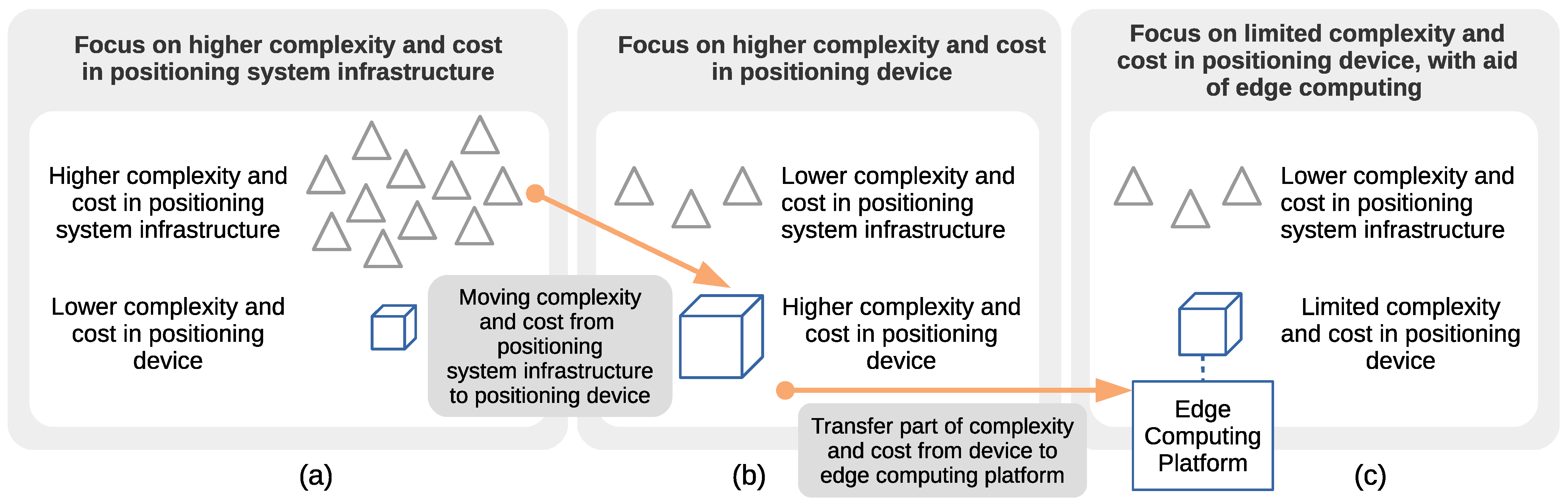


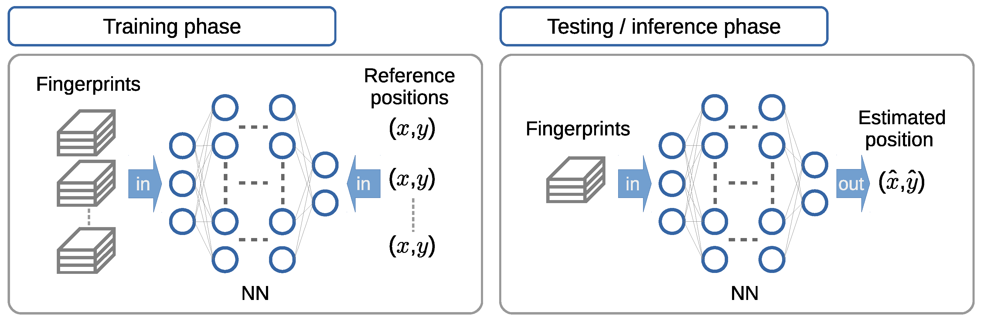
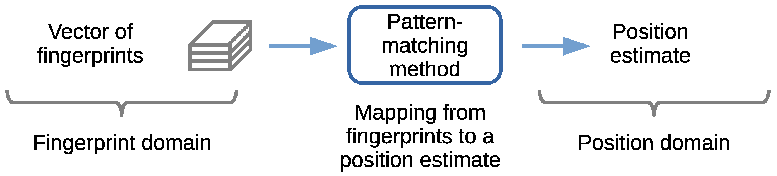
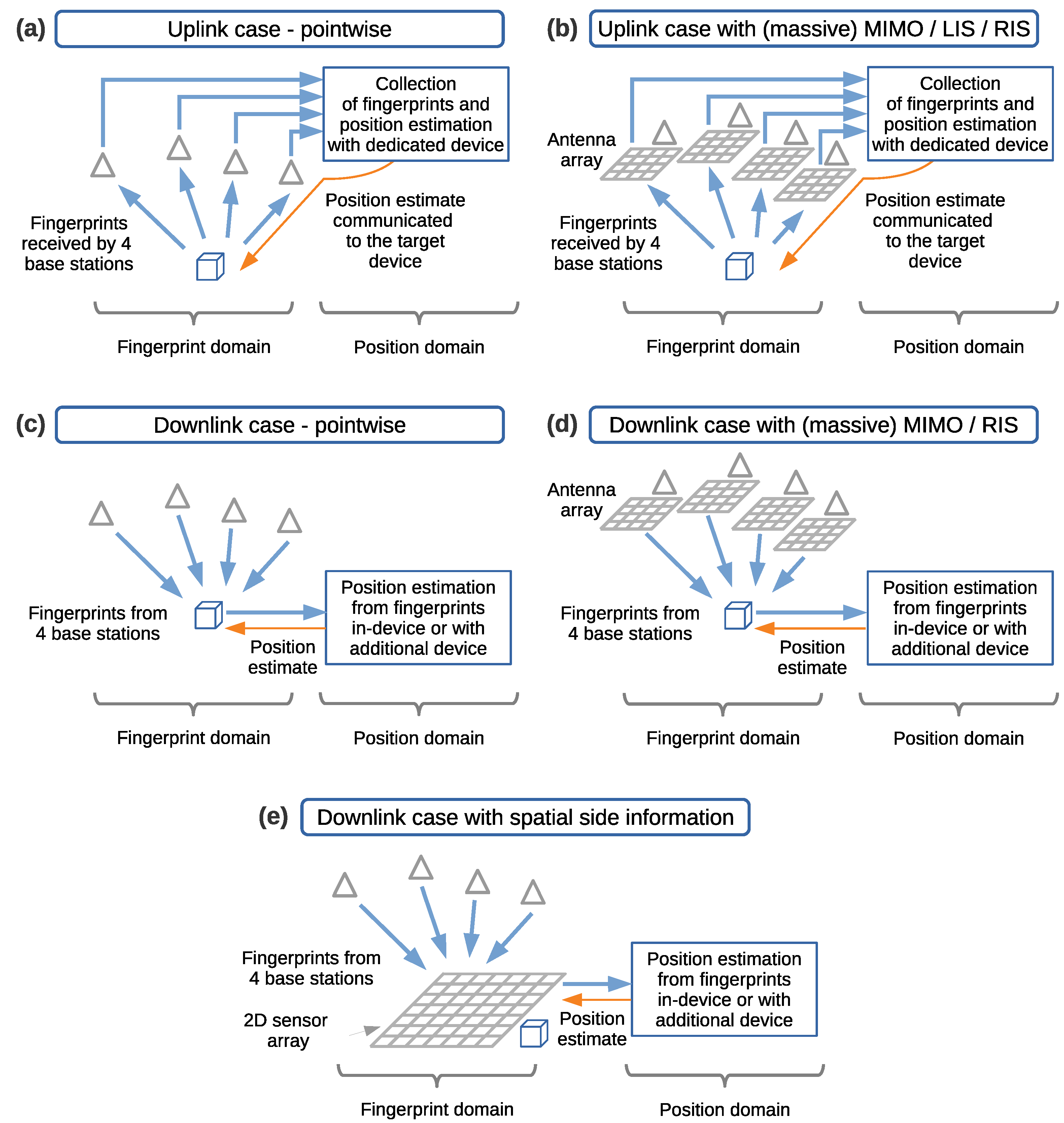
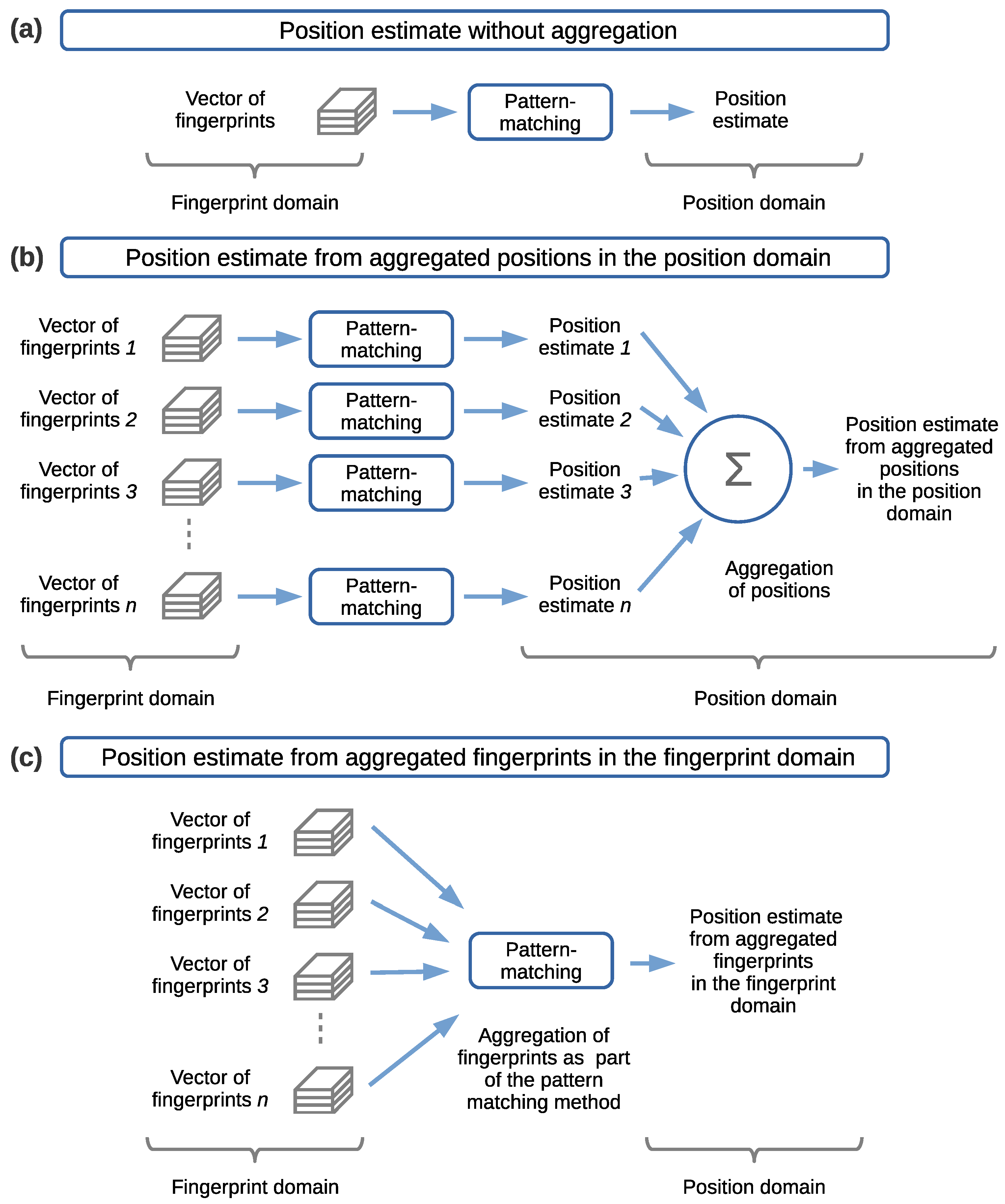
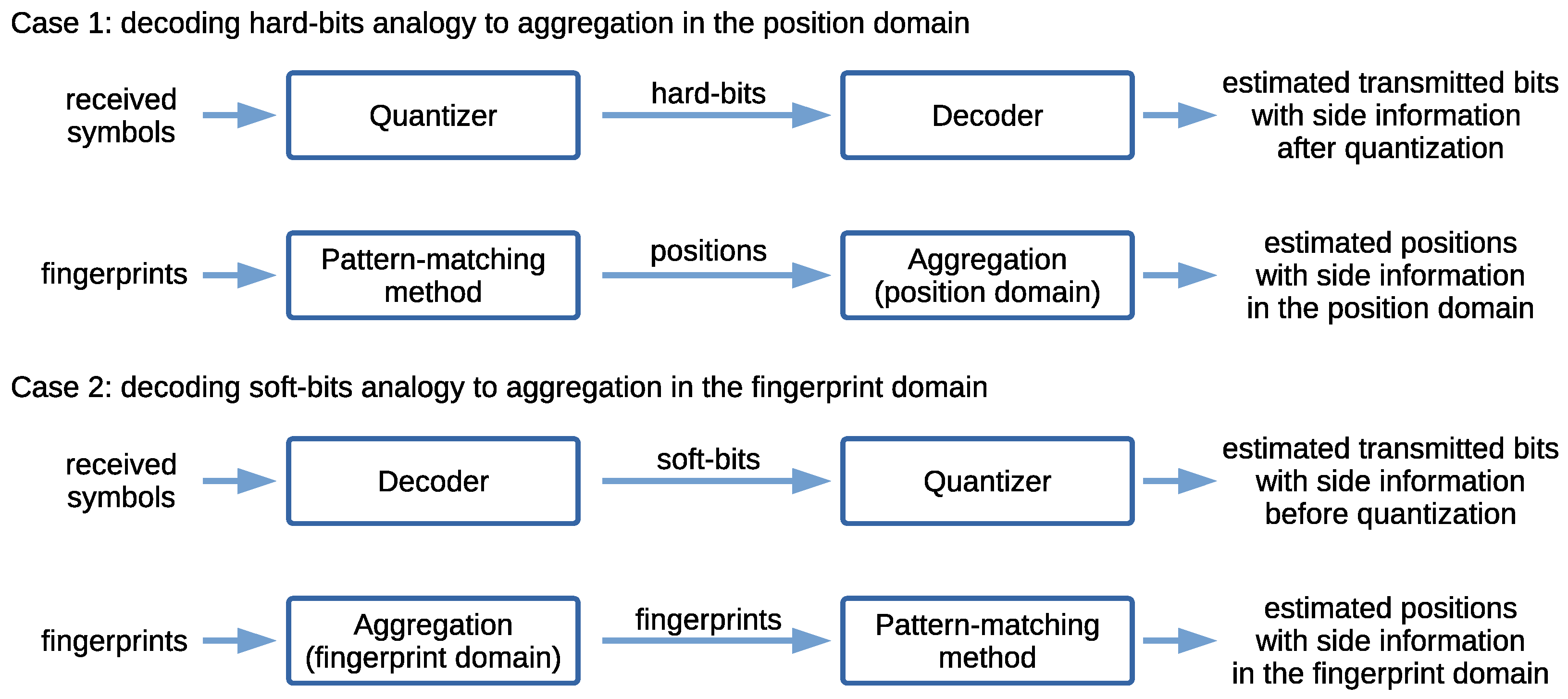

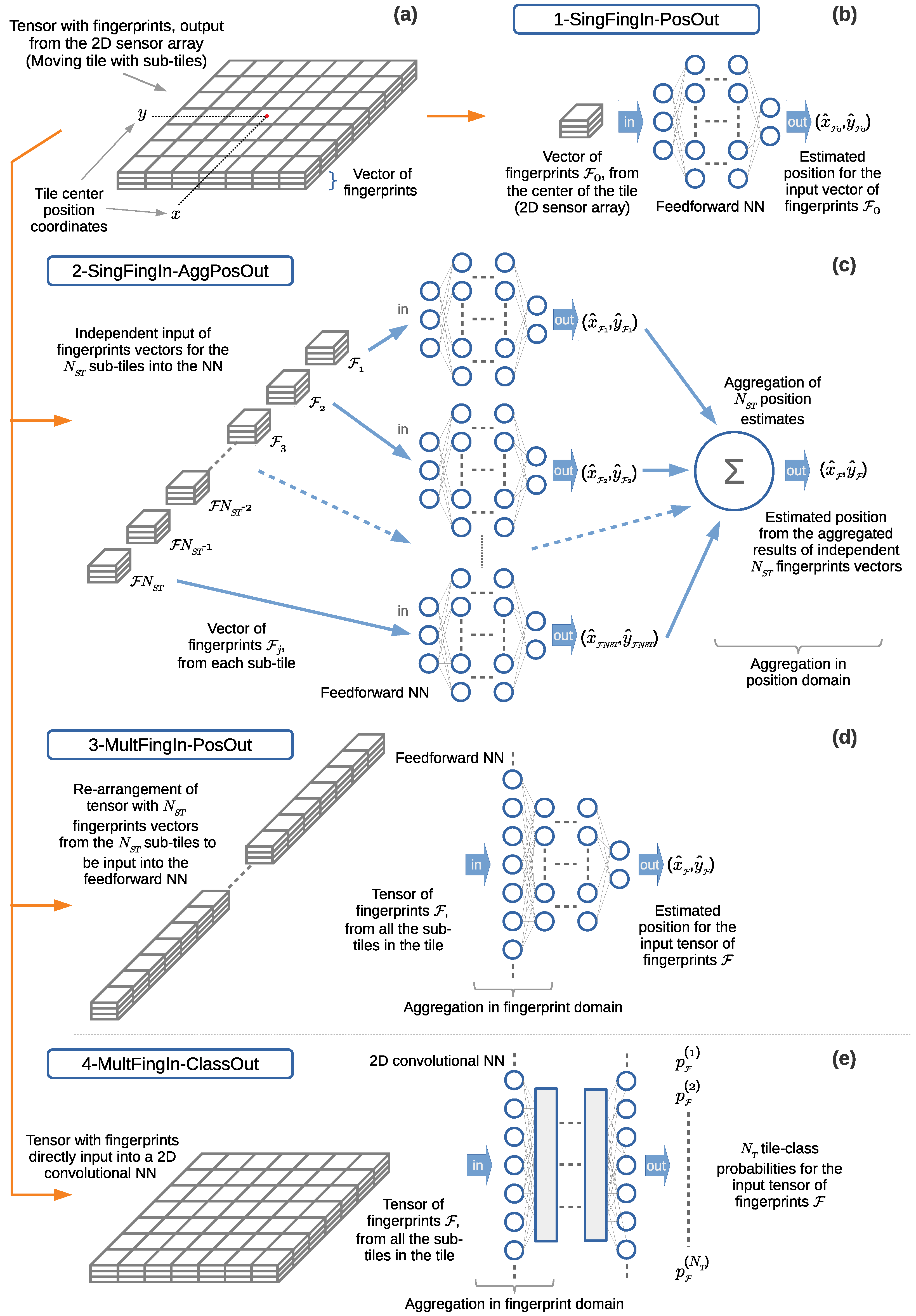
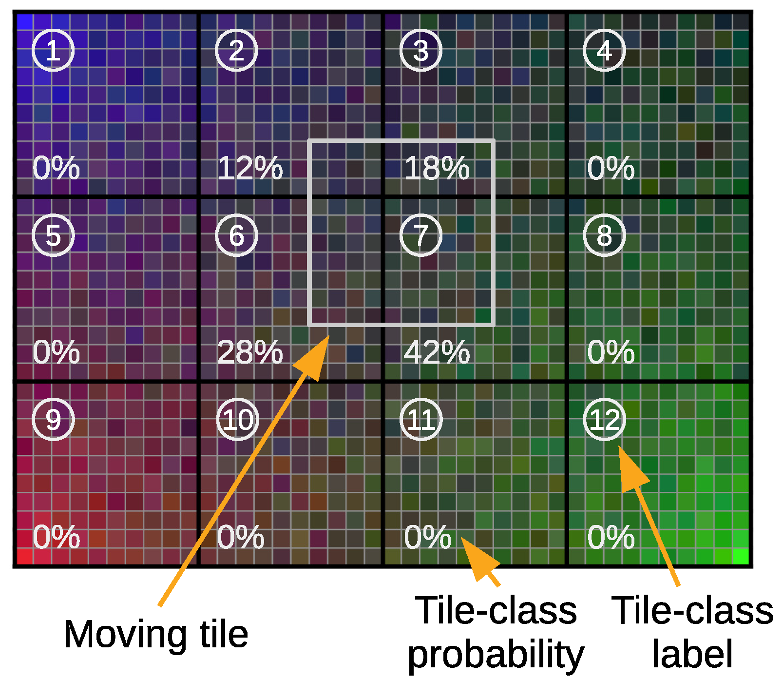

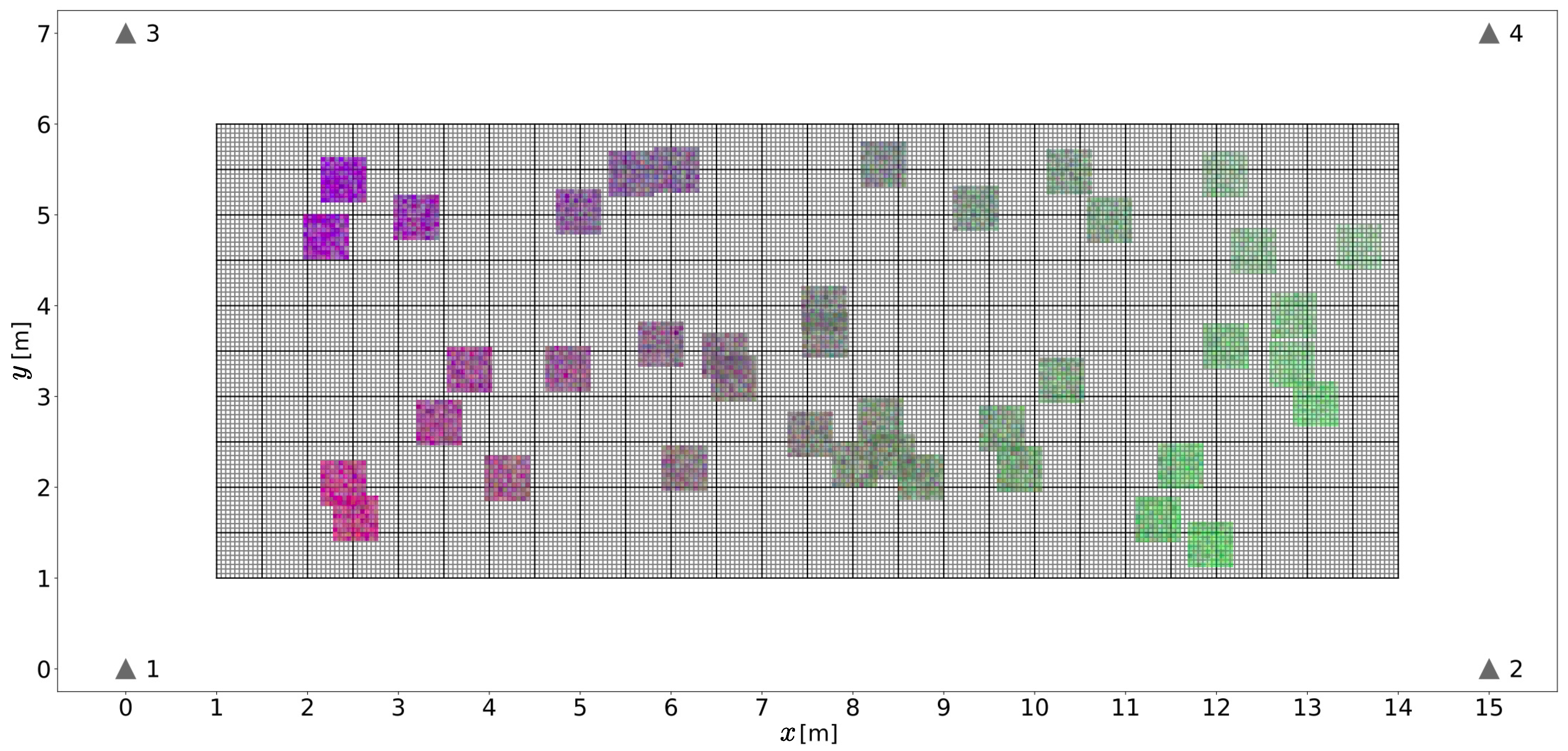
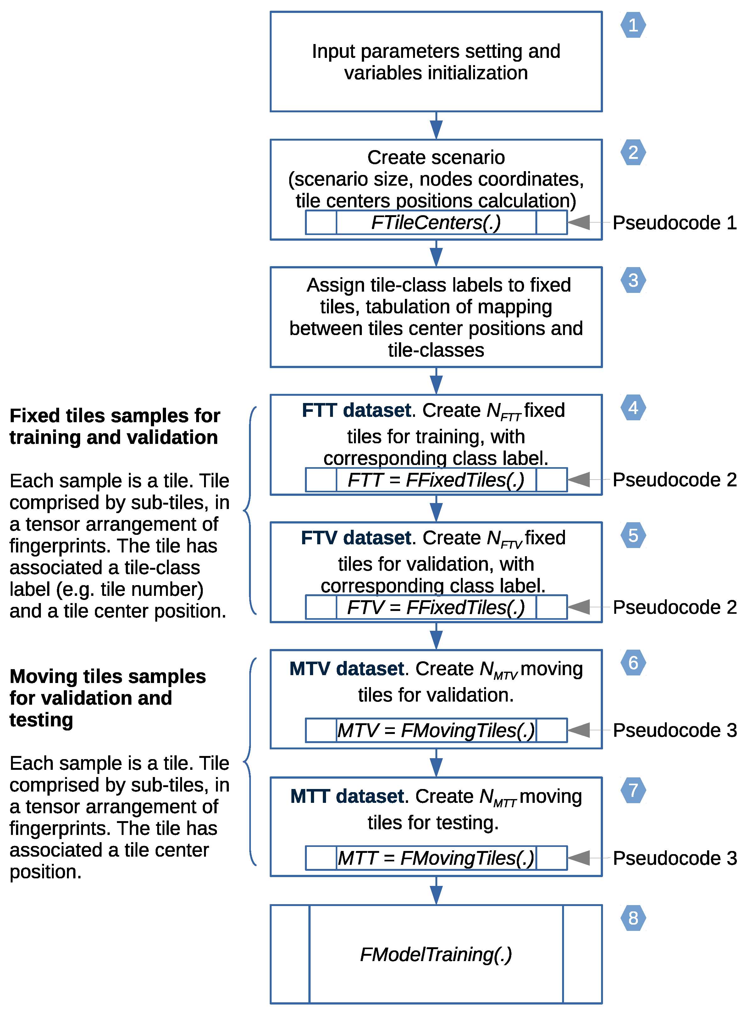
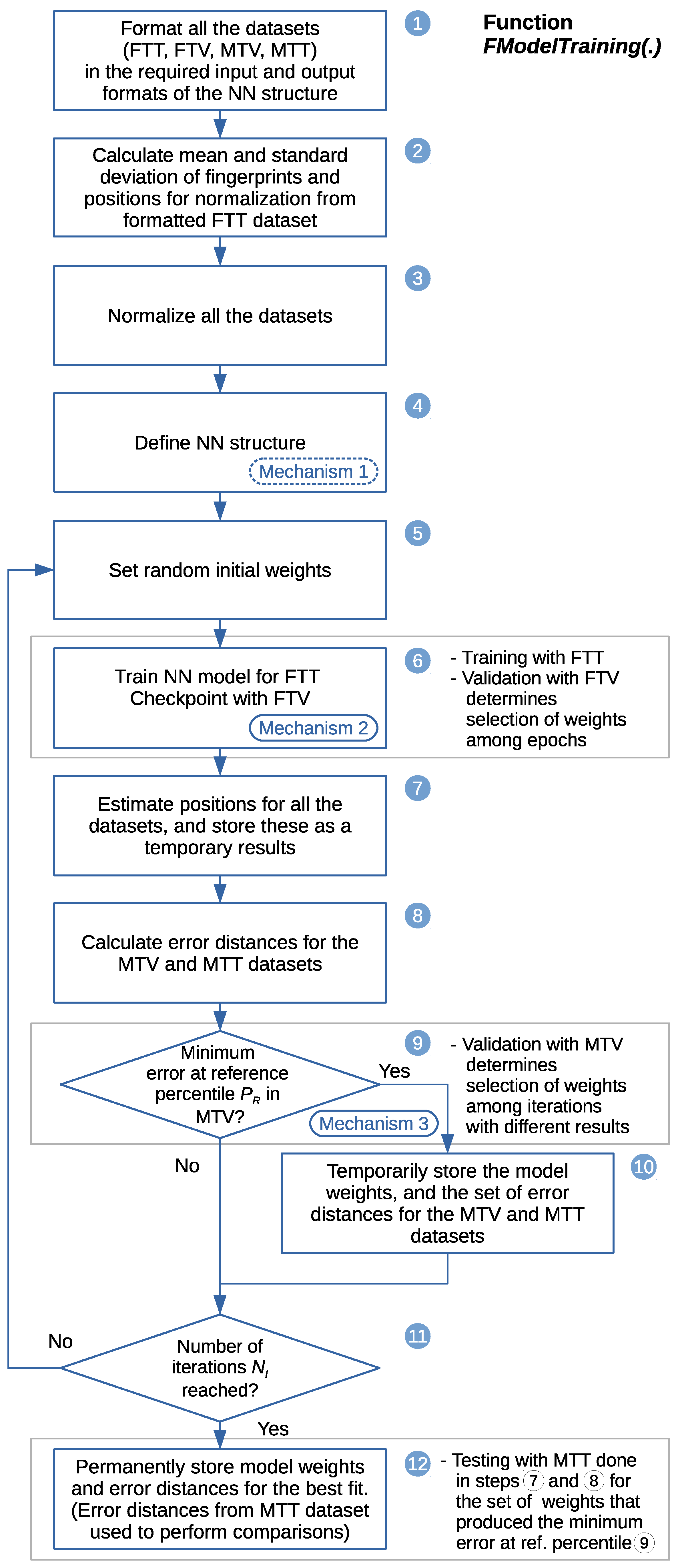

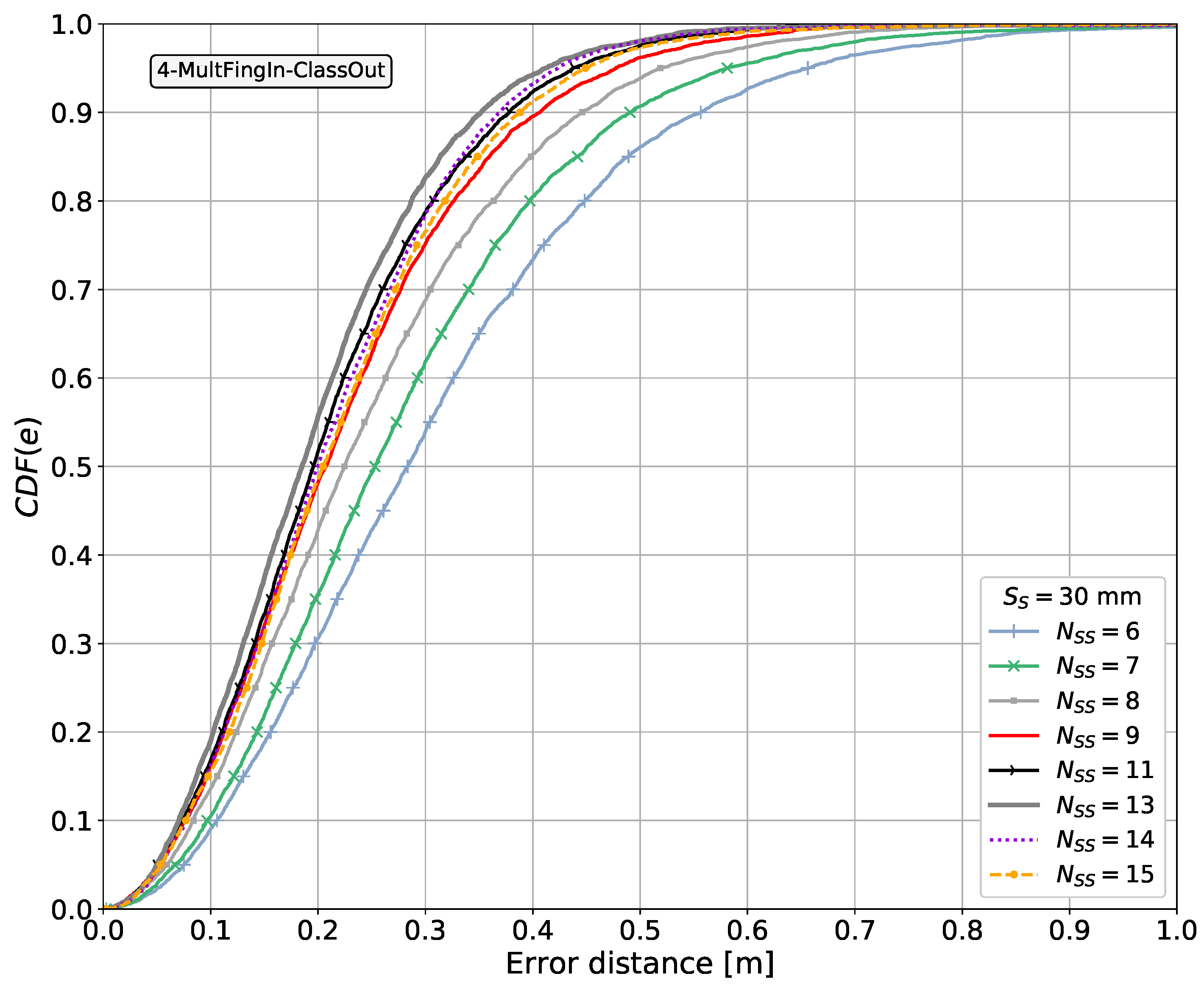
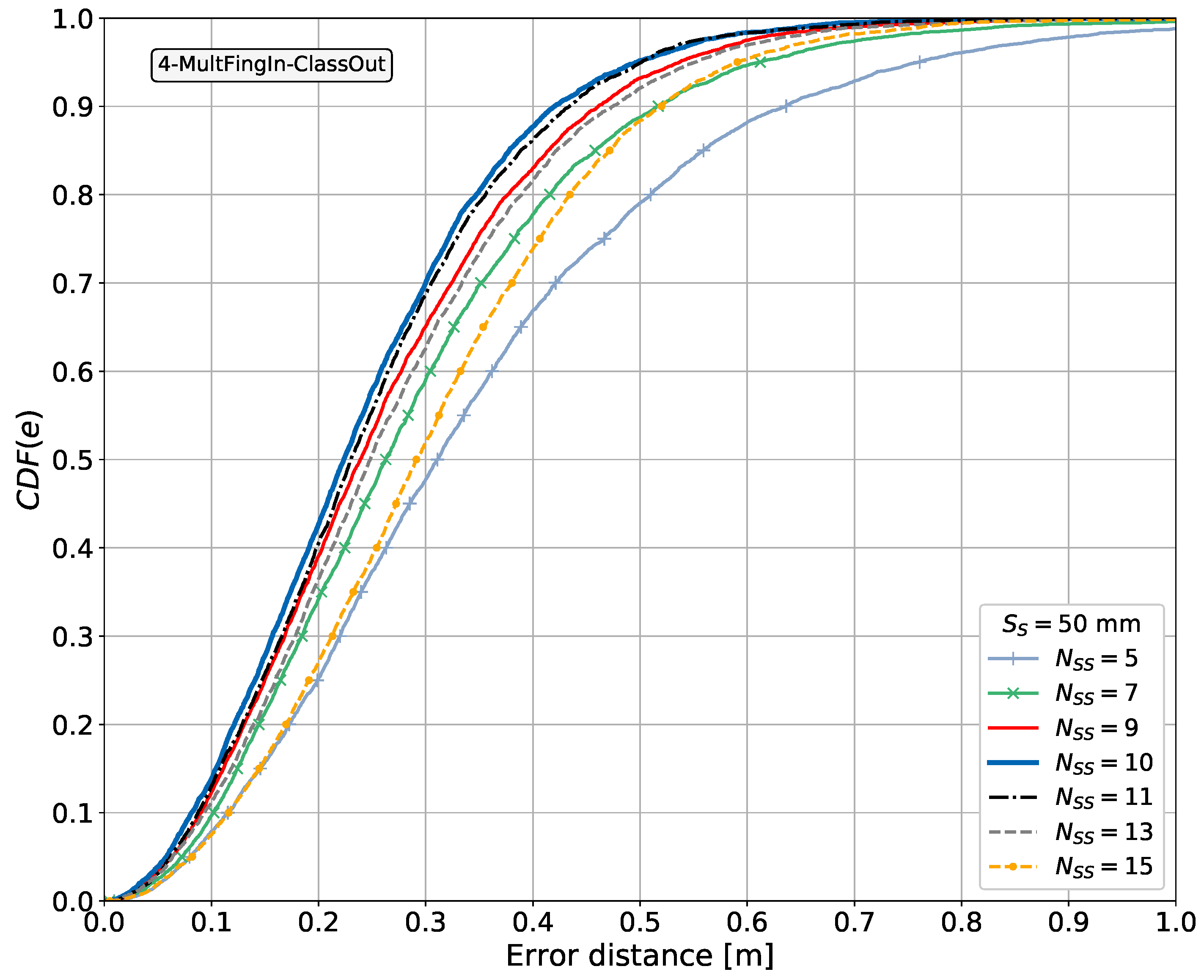
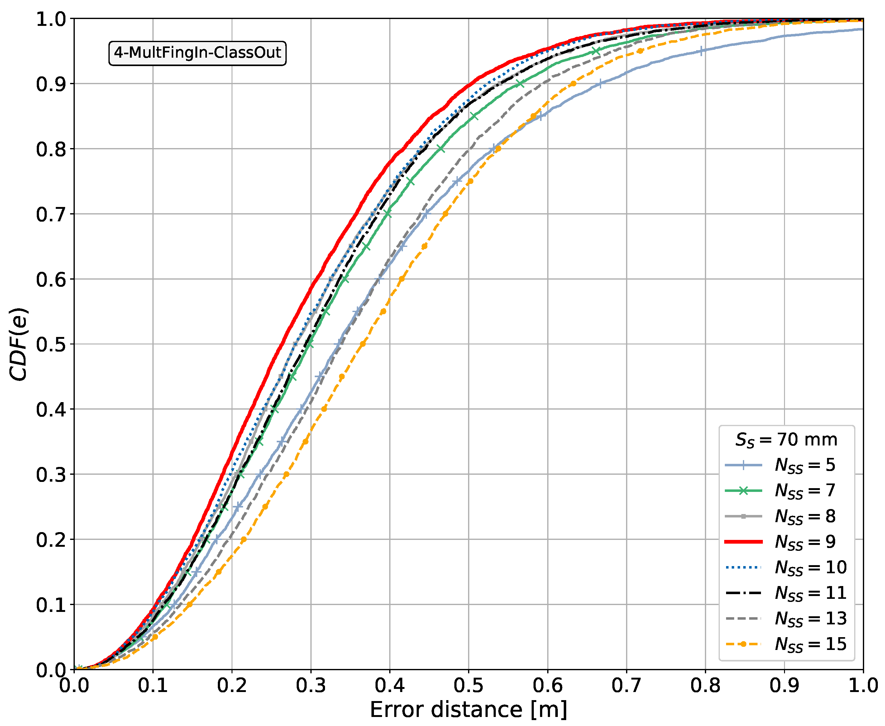
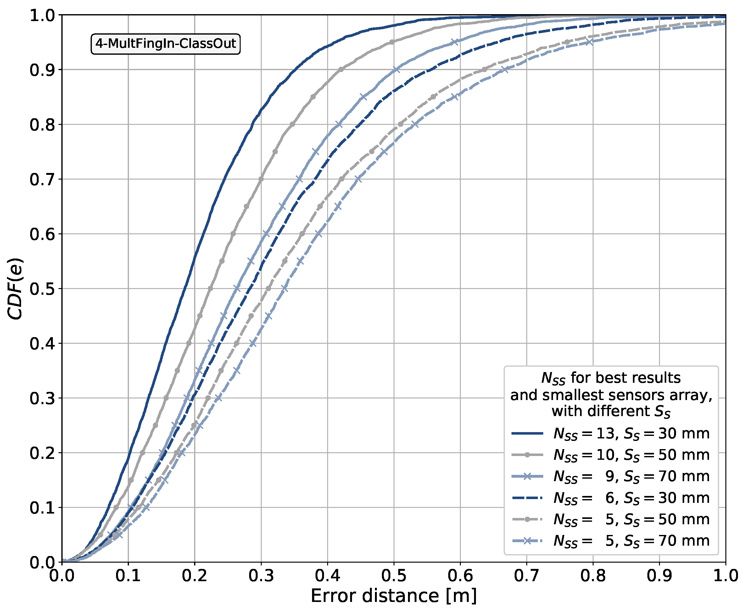
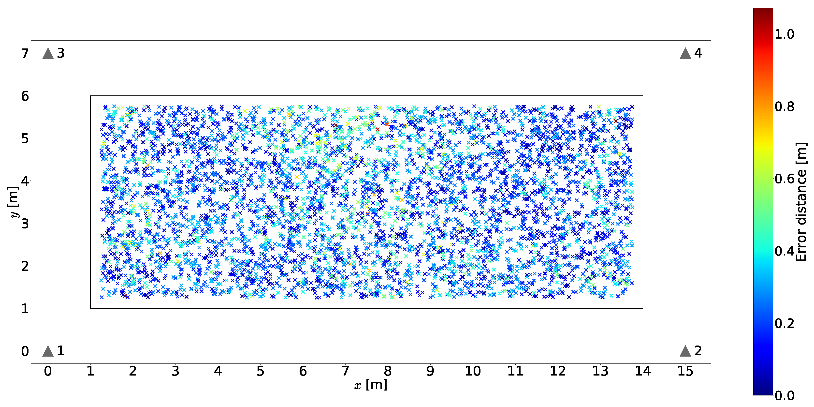
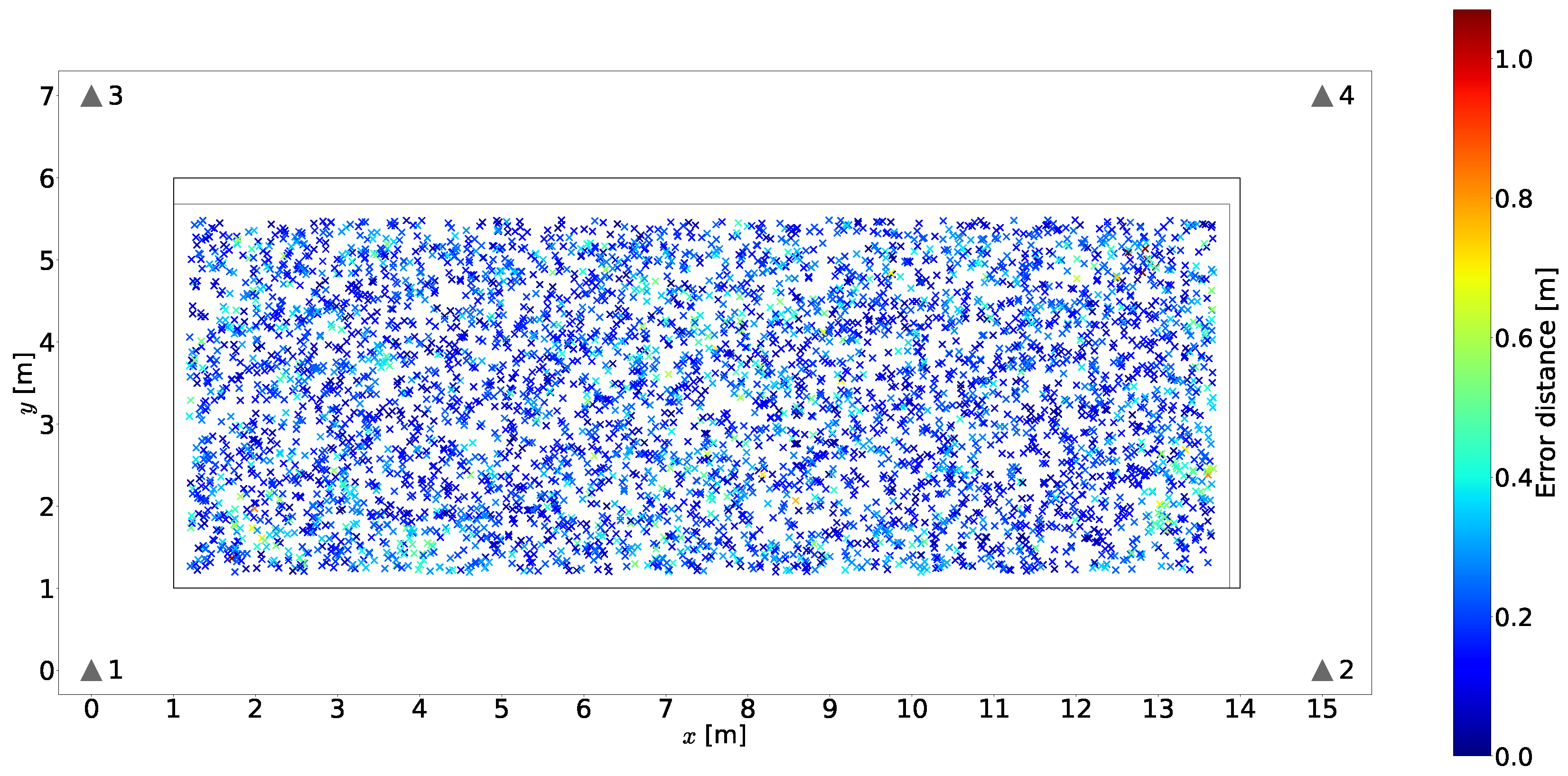
Disclaimer/Publisher’s Note: The statements, opinions and data contained in all publications are solely those of the individual author(s) and contributor(s) and not of MDPI and/or the editor(s). MDPI and/or the editor(s) disclaim responsibility for any injury to people or property resulting from any ideas, methods, instructions or products referred to in the content. |
© 2025 by the authors. Licensee MDPI, Basel, Switzerland. This article is an open access article distributed under the terms and conditions of the Creative Commons Attribution (CC BY) license (https://creativecommons.org/licenses/by/4.0/).