Article

Carbon Emissions, Health Expenditure, and Economic Effects on Life Expectancy in Malaysia

by
Norkhairunnisa Redzwan
1,2 and
Rozita Ramli
1,*
1
Department of Mathematical Sciences, Faculty of Science and Technology, Universiti Kebangsaan Malaysia, Bangi 43600, Malaysia
2
School of Mathematical Sciences, College of Computing, Informatics and Mathematics, Universiti Teknologi MARA, Shah Alam 40450, Malaysia
*
Author to whom correspondence should be addressed.
World 2024, 5(3), 588-602; https://doi.org/10.3390/world5030030
Submission received: 31 May 2024 / Revised: 22 July 2024 / Accepted: 23 July 2024 / Published: 30 July 2024

Abstract

:
Population aging, urbanization, and life expectancy are among the main pillars of sustainable economic, social, and environmental development of the future, as outlined by the Sustainable Development Goals (SDGs) of the United Nations. Globally, the current population structure exhibits an increasing proportion of the elderly along with rising healthcare costs and climate change. Malaysia faces a similar experience, where 14% of its population is expected to account for the elderly by 2030. To achieve the SDGs, attention should be given to their pillars, namely life expectancy, health expenditure, economic development, and carbon emissions. Limited research that addresses these key factors has been conducted, especially in emerging economies, such as Malaysia. Therefore, this study aims to contribute to the existing literature by analyzing the long-term and short-term relationships between carbon emissions, GDP, health expenditure, and life expectancy in Malaysia. The autoregressive distributed lag (ARDL) bounds cointegration test was adopted to determine the long-term and short-term effects on life expectancy from 1997 to 2021. The findings indicate that cointegration existed among the variables, and carbon emissions and health expenditure had a statistically significant relationship with life expectancy in the short run. Hence, greater attention should be paid to these two factors, particularly in the short term, to ensure that Malaysia can maintain the health and well-being of the nation in line with the SDG requirements.

1. Introduction

An aging population refers to the significant growth in the number of aged people relative to younger generations. It is a global phenomenon impacting numerous nations. In 2019, 703 million persons worldwide were estimated to be 65 years of age or older [1]. It is projected that the senior population, defined as those aged 65 years and older, will comprise 1.5 billion persons by 2050. People are able to live longer and experience better living as a result of technological advancements and improvements in healthcare facilities. This situation, combined with declining fertility, rising life expectancy, and rural-to-urban migration, all significantly contribute to population aging. For example, rural areas experience faster aging due to the rural-to-urban migration of the younger generation. Rapid aging is also caused by urbanization due to lower fertility and mortality rates in urban populations [2]. Population aging provides an opportunity for economic growth because of improved health and well-being, which subsequently contribute to better labor force participation and productivity [3]. An aging workforce is valuable in works involving experience, knowledge, and profound managerial capabilities as compared with jobs needing intense physical strength [4]. However, population aging is not without challenges. Owing to the imbalance between the active workforce and the retired elderly population, an increase in the size of the aging population will have an impact on the viability of social security and pension systems [3]. More resources are also required to provide for old age care to ensure that the senior population can experience a better quality of life. Managing resource allocation is crucial because the impact of population aging differs between urban and rural areas [2,3]. Essentially, to ensure the good health and well-being of the increasingly aged population, collaboration across different sectors is crucial because, ultimately, population aging, population growth, international migration, and urbanization significantly influence sustainable economic, social, and environmental development in the future.
In 2018, 55% of people lived in cities, and that number is expected to rise to 68% by 2050 [5]. Urban population growth is attributed to migration to places with better socioeconomic and health conditions, including jobs, access to healthcare, education, and the conversion of rural areas into urban areas [6,7]. Urbanization negatively impacts social conduct, the environment, and human health. Rapid industrial development in urban areas leads to increased emissions of greenhouse gases and other pollutants, resulting in climate change. Urbanization also results in decreases in natural resources, like food, water, and land, to meet the demands of the urban population [6,8,9,10]. More land needs to be developed for urbanites’ dwellings, agriculture, and waste management. The primary causes of social conduct problems brought by urbanization are the urban poor, who live in places with generally higher living standards than those in rural areas, and the urban lifestyle, which can be subjected to prolonged stress and strain. Urban poor people are less resistant to sickness due to their financial and socioeconomic hardships [9,11]. Health problems, encompassing both physical and mental health, are other issues associated with urbanization. Urban inhabitants are more likely to be exposed to risk factors for noncommunicable diseases, like diabetes, cardiovascular disease, and depression, because of their urban lifestyle [7,12]. Their increased susceptibility to communicable diseases is also due to metropolitan areas’ high population density and overcrowding [13]. According to [8], a direct link was found between the number of confirmed cases during the recent COVID-19 pandemic and the size of the urban population. Thus, infectious illness risks might be increased by the dense population in metropolitan settings.
Life expectancy measures the health and well-being of a nation and is one of the pillars of the Sustainable Development Goals (SDGs). The SDGs, particularly SDG 3, SDG 7, and SDG 13, were developed by the United Nations to extend life expectancy by reducing environmental pollution and allowing access to inexpensive clean energy for everyone [14,15]. Other pillars of the SDGs include healthcare expenditure, economic development, and carbon emissions [16]. As part of the effort to achieve the SDGs by 2030, attention should be paid to these pillars and to establishing the existence of long-term relationships among these variables. Although many studies have focused on various SDG pillars [17,18,19,20,21,22], empirical studies that incorporate these primary pillars are rather limited, particularly in emerging economies such as Malaysia. In Malaysia, life expectancy exhibited an increasing trend over the past few decades, surpassing global life expectancy. The Department of Statistics Malaysia (DOSM) predicts that, by 2050, 14.5% of Malaysia’s population will consist of persons aged 65 and above [23]. Similar increasing trends are seen in Malaysia’s healthcare expenditure, GDP, and carbon dioxide (CO2) emissions, which highlights the importance of capturing the cointegration of these determinants. Therefore, this study aims to contribute to the existing literature by determining the effects of health expenditure, GDP, and CO2 emissions on life expectancy at birth in an emerging economy, such as Malaysia. Our findings indicate that cointegration exists among the variables, and CO2 emissions and health expenditure have a statistically significant relationship with life expectancy in the short term. The findings of this study are essential, as they show that health resources and environmental factors affect life expectancy in the short term. Hence, special attention should be paid to these factors to achieve the SDGs. Several policy recommendations were drawn, particularly to emphasize the importance of policies on the health and well-being of the population while shifting towards renewable energy as an effort to reduce environmental degradation.
The remainder of this paper is organized as follows: Section 2 describes the literature review, Section 3 describes the material and methods, Section 4 discusses the results, and Section 5 concludes the paper.

2. Literature Review

2.1. Introduction

Life expectancy is a measure of the health and well-being of a nation. Life expectancy at birth indicates the number of years a newborn is expected to live. Figure 1 illustrates the comparison of the historical trend of life expectancy in Malaysia, the East Asia and Pacific region, and the world.
Based on Figure 1, Malaysia’s life expectancy is greater than the global life expectancy. The advancement in technology and improved healthcare facilities allow individuals to live longer and experience better lives. This situation, combined with declining fertility, rising life expectancy, and rural-to-urban migration, all significantly contribute to population aging. Global life expectancy increased from 62.2 years in 1980 to 71.3 years in 2021, while Malaysia’s life expectancy increased from 68.2 years in 1980 to 74.9 years in 2021. Thus, on average, the population of Malaysia is expected to live up to 74.9 years old in 2021. By 2030, 14.5% of Malaysia’s population is projected to be elderly people aged 65 and above, and Malaysia is projected to be on the path of becoming an aging population. Although Malaysia’s life expectancy has improved over the years, exceeding the global and regional life expectancies, it is worth noting that from 2009, Malaysia experienced a lower life expectancy as compared to the region. Several studies were conducted to analyze the relationship between life expectancy and its determinants in Malaysia. For example, reference [25] found that between 1960 and 2014, Malaysia’s life expectancy was positively influenced by economic growth and real import and export per capita. Reference [26] concluded that between 1995 and 2017, an increase in GDP per capita, health expenditure, and population increased Malaysia’s life expectancy, while CO2 emissions reduced life expectancy. Moreover, Refs. [27,28] found that life expectancy can be affected by health resources, environmental, and macroeconomic factors. Macroeconomic and health resource factors such as GDP and total health expenditure were found to have a positive impact on life expectancy [22].

2.2. Pillars of Sustainable Development

A holistic sustainable development encompasses several areas such as developments in the economy, social health and well-being, and environment. In the past decades, studies have shown that health resources, environmental, and economic factors are consequences of urbanization [2,7,8,9]. Urbanization is defined as people moving from rural to urban areas primarily for better employment opportunities and searching for improved standards of living. Migration from rural to urban areas is also due to better education and health facilities, as well as public infrastructures [6,7]. Furthermore, rising urbanization has substantial effects on health resources such as limited healthcare facilities and unsanitary living conditions. Urban populations, particularly children and the elderly, are more at risk of poor air quality due to their fragile immune systems [9]. In the context of economic growth and the environment, an increase in urban population attracts industrialization and investment opportunities, resulting in higher CO2 emissions through fossil fuel consumption [6].
In this study, we develop a relationship framework, as shown in Figure 2, which describes the relationship between urbanization and life expectancy in terms of health resources, the environment, and economic development.
Health resources, such as health expenditures, the number of health personnel, health facilities, and vaccinations, are some of the main factors affecting life expectancy. In this study, we focus on health expenditures. In general, health expenditures can be classified into three categories: public, private, and out-of-pocket expenditures. Public and private health expenditures refer to expenditures incurred by the government and private institutions, respectively. Out-of-pocket expenditures refer to expenditures incurred by households or individuals. Health expenditures include curative and rehabilitative care, long-term nursing care, medical facilities, education and training of health personnel, research and development in health, and other health-related expenditures [29]. Reference [22] has shown that health expenditures have a positive impact on life expectancy, where an increase in health expenditure can potentially increase life expectancy. The study showed that life expectancy in Singapore, Malaysia, and Thailand was positively affected by healthcare resources which include the number of medical personnel, healthcare expenditure, and vaccination. However, in the Eastern Mediterranean, reference [30] indicated no significant relationship between healthcare expenditure and life expectancy due to the socioeconomic status of the region. Another measure of demographic indicator besides life expectancy is mortality. Reference [31] showed that out-of-pocket health expenditures have a positive and statistically significant effect on the mortality of Malaysian children under five years old, and Ref. [32] highlighted that a 1% increase in health expenditure per capita can reduce 0.5% and 0.35% of under-five and maternal mortality in Sub-Saharan Africa, respectively.
Environmental development, including emissions of pollutants, leads to adverse impacts on life expectancy. CO2 derived from fossil fuel combustion, transportation, industrialization, and electricity generation is one of the main greenhouse gases that affect climate change. CO2 emissions have been widely used as a measure of environmental degradation. References [33,34] highlighted that population growth and the aging population contributed to an increase in carbon emissions. For example, as the population increases, more energy is being produced for industrialization and electricity, which results in more carbon emissions. Rising carbon emissions can reduce the health condition of the population. Previous studies have shown similar results across different countries, where carbon emissions have negative effects on life expectancy [15,26,35]. Furthermore, reference [36] mentioned that air pollutants, specifically PM2.5, have a greater impact on life expectancy for states that have higher income inequality. A recent study [19] on the most polluted countries in regions of Asia, Africa, South America, and Europe found that there is an inverse impact of pollution on life expectancy. The severity of the impact varies between countries based on income level and access to healthcare facilities. The study was conducted in 31 countries from 2000 to 2017 and highlighted the effects of carbon emission, GDP per capita, health spending, clean water, and sanitation on life expectancy. Reference [20] examined the association between CO2 emission and GDP with life expectancy in Southeastern Europe. Along with other factors, reference [20] concluded that health expenditure as a percentage of GDP has significant effects on life expectancy as compared to out-of-pocket healthcare expenditure.
GDP is commonly used as an indicator of economic growth and development. References [22,37] highlighted that GDP has a positive and statistically significant relationship with life expectancy in Brazil, Malaysia, Singapore, and Thailand. However, the relationship is statistically insignificant in other developing countries [22]. Similar findings were reported in [26,30], showing that favorable economic growth can increase life expectancy. Reference [26] investigated the relationship between life expectancy, GDP, carbon emissions, and health expenditure in D-8 countries from 1992 to 2017, and it was found that other factors that positively affect life expectancy are population and healthcare expenditure. A study [30] in the Eastern Mediterranean region from 1995 to 2007 found that other factors that positively affect life expectancy are employment, education, urbanization, and food availability. Reference [36] also reported that GDP has a negative and statistically insignificant relationship with life expectancy. This means that a change in GDP may not have a direct impact on the change in the life expectancy of a population.
Previous studies have established CO2 emission, GDP, and healthcare expenditure as the determinants of life expectancy in many regions across the globe, including Southeastern Europe, Asia, and Africa [17,18,19,20,21,22]. Although abundant literature is available on this topic, limited studies have incorporated these three determinants in a single model to determine factors affecting life expectancy, particularly in emerging and developing economies. For example, Refs. [17,20] examined factors affecting life expectancy which are limited to CO2 emission and GDP, while Ref. [21] was limited to life expectancy, CO2 emission, healthcare expenditure, and energy-related factors in Nigeria. Their findings indicate an inverse relationship between CO2 emission and healthcare expenditure with life expectancy. Reference [20] analyzed the causal relationship between GDP, CO2 emissions, and life expectancy in Turkey from 1960 to 2018. The study proposed reducing dependence on non-renewable energy as part of steps to achieve sustainable development. Therefore, this study aims to link these three important determinants by extending the works of [17,20,21] to incorporate all three factors into an empirical model to model the factors affecting life expectancy.

3. Methodology

This section explains the data used in the study and methodology to estimate the long-run and short-run coefficients by using the ARDL model. Furthermore, this section describes the model diagnostic tests used to check for the goodness of fit of the model.

3.1. Data and Description of Variables

This study aims to determine the effects of health resources, and environmental and economic factors on Malaysia’s life expectancy from 1997 to 2021. Health expenditure was used as a proxy for health resources, while GDP and CO2 emissions were proxies for macroeconomic and environmental factors, respectively [28]. We adopted life expectancy as the dependent variable, whereas we adopted health expenditure, GDP, and CO2 emissions as the independent variables. Following the works of [38], GDP per capita was employed as an indicator of economic development. Economic development is important to ensure a universal approach to improve the standard of living and decrease the level of poverty. Alternatively, economic growth represents the increase in a nation’s wealth over time as indicated by the increase in national income and output [39,40]. To obtain per capita values, the variables were divided by population data obtained from the Department of Statistics (DOSM) [23]. Annual data were obtained from online databases of DOSM, the Ministry of Health Malaysia, and the World Bank. The description of variables is shown in Table 1. We used the autoregressive distributed lag (ARDL) bounds cointegration test via the ARDL package [41] in R statistical programming language version 4.2.2 [42].
Therefore, we proposed a model that analyzes the effects of health expenditure, GDP, and CO2 emissions on life expectancy as follows:
L E t = α + β 1 H E t + β 2 G D P t + β 3 C O 2 t + ϵ t
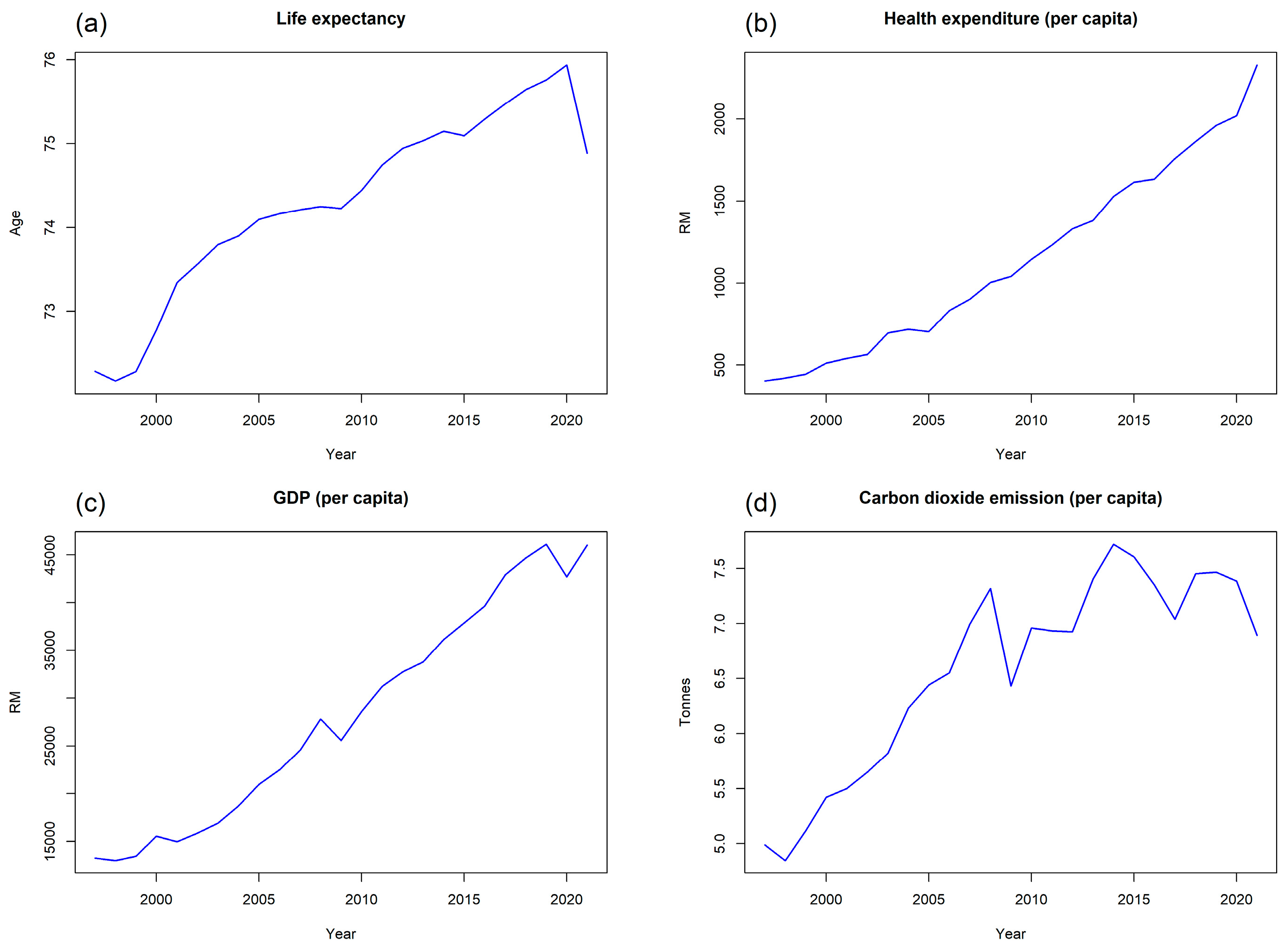
In Equation (1), L E t is the natural logarithm of life expectancy at birth at time t , H E t is the natural logarithm of total health expenditure at time t , G D P t is the natural logarithm of GDP per capita at time t , C O 2 t is the natural logarithm of CO2 emissions per capita at time t , and ϵ t is the error term that is independent and identically distributed with mean 0 and constant variance. Figure 3 below shows the plot of each variable used in this study.
Based on Figure 3, all the variables show an upward trend from 1997 to 2021. For CO2 emissions, a steep incline was recorded between 1997 and 2007/2008. It is interesting to note that in 2020, there was a sharp decline in life expectancy, GDP per capita, and CO2 emissions per capita, while total health expenditure per capita recorded a steep increase, as in 2020, the COVID-19 pandemic affected Malaysia. During the pandemic, many people were infected with the virus, and in serious cases, this resulted in deaths. Hence, a huge amount of health expenditure was allocated for the treatment of COVID-19 patients. The slowdown of economic activities and industrialization during the pandemic resulted in a decrease in GDP and less CO2 emissions.

3.2. Autoregressive Distributed Lag (ARDL) Bounds Test for Cointegration

In this study, we applied the autoregressive distributed lag (ARDL) bounds cointegration test to find the long-run relationship between variables. The ARDL model contains lags of the dependent and independent variables. It is a standard least square regression model that is denoted by A R D L ( p ,   q 1 ,   ,   q k ) , where p is the lag of the dependent variable and q i is the lag of ith independent variable. The advantages of the ARDL model are as follows: (1) it can be applied to I(0) or I(1) time series or a combination of both, (2) it can be used to determine both short-run and long-run estimates, and (3) it is widely used to determine cointegration of variables [31,45,46,47,48].
Since this method requires that none of the variables is integrated at the order I(2), unit root tests such as the Phillips–Perron test [49] with a null hypothesis of nonstationarity were performed on the variables at its level and first difference values. As a supplementary test, the Kwiatkowski–Phillips–Schmidt–Shin (KPSS) test [50] with the null hypothesis of stationarity was also conducted.
The ARDL bounds test for cointegration involves two steps. The first step is to determine the existence of long-run relationships among all variables. The second step is to obtain the long-run and short-run estimates of the ARDL model, and the speed of adjustment of the long-run equilibrium. Therefore, the A R D L ( p ,   q 1 ,   ,   q k ) model between life expectancy, health expenditure, GDP, and CO2 emissions is as follows:
L E t = α 0 + i = 1 p 1 γ 0 , i L E t i + j = 0 q 1 1 γ 1 , j H E t j + j = 0 q 2 1 γ 2 , j G D P t j + j = 0 q 3 1 γ 3 , j C O 2 t j + θ 1 L E t 1 + θ 2 H E t 1 + θ 3 G D P t 1 + θ 4 C O 2 t 1 + ϵ t
where is the first difference operator, L E t is the natural logarithm of life expectancy at birth at time t , H E t is the natural logarithm of total health expenditure at time t , G D P t is the natural logarithm of GDP per capita at time t , C O 2 t is the natural logarithm of CO2 emissions per capita at time t , and ϵ t is the error term at time t .
The selection of lags in the A R D L ( p ,   q 1 ,   ,   q k ) model is based on the partial autocorrelation function (PACF) plot, Akaike Information Criterion (AIC), and Bayesian Information Criterion (BIC). Based on the PACF plot, several A R D L ( p ,   q 1 ,   ,   q k ) models were compared, and the one with the lowest AIC and BIC was chosen as the best model.
During the first stage of the ARDL cointegration test, the null hypothesis, H 0 , of no cointegration is analyzed based on F-statistic following [51] on Equation (2). The null hypothesis is rejected when the F-statistic is greater than the upper bound of the critical value for k + 1 number of variables, which means that there is cointegration between the variables. The null hypothesis fails to be rejected if the F-statistic is less than the lower bound of the critical value, which means that there is no cointegration between the variables. However, if the F-statistic falls between the lower and upper bound of the critical value, it indicates that the result is inconclusive [46]. The hypothesis for the bounds cointegration test is as follows:
H 0 :   θ 1 = θ 2 = θ 3 = θ 4 = 0   ( no   cointegration )
H 1 : θ 1 θ 2 θ 3 θ 4 0 ( cointegration   exists )
In the second stage, the long-run and short-run estimates of the ARDL model and the speed of adjustment of the long-run equilibrium are determined. The long-run equation, also known as the cointegrating cointegration, and the short-run equation are represented by Equations (5) and (6), respectively.
L E t = π 1 + π 2 H E t + π 3 G D P t + π 4 C O 2 t + ϵ t
L E t = i = 1 p 1 γ 0 , i L E t i + j = 0 q 1 1 γ 1 , j H E t j + j = 0 q 2 1 γ 2 , j G D P t j + j = 0 q 3 1 γ 3 , j C O 2 t j + φ E C T t 1 + ε t
where E C T t is the error correction term (ECT) at time t ; φ is the coefficient of ECT, also known as the speed of adjustment to equilibrium; and ε t is the error term.
The speed of adjustment, φ , is obtained by estimation of Equation (6) after the inclusion of E C T t 1 into the model. It indicates the speed at which variables adjust to the equilibrium once it deviates from the long-run equilibrium. According to [45], the coefficient φ should have a negative sign and be statistically significant. In this study, A R D L ( p ,   q 1 ,   ,   q k ) model estimation was conducted using the “ARDL” package [41] in R statistical computing language.

3.3. Model Diagnostic

To check for the goodness of fit of the model, we conducted a diagnostic check on the A R D L ( p ,   q 1 ,   ,   q k ) model. A serial correlation test, normality test, and heteroscedasticity test for the residuals were determined by using the Durbin–Watson, Jarque–Bera, and Breusch–Pagan tests, respectively.

4. Results and Discussion

4.1. Unit Root Test

It is imperative to test the stationarity of each variable to fulfill the requirement of the ARDL bounds cointegration test. This method requires that none of the variables is integrated at order I(2). We conducted Phillips–Perron (PP) and KPSS stationarity tests to check for the stationarity of these variables. The null hypothesis of the PP test is the time series is stationary, while the null hypothesis of the KPSS test is the time series is not stationary.
Table 2 below shows the results of unit root tests for each variable. All variables are significant after the first difference, and the null hypothesis of stationarity for the PP test is rejected. For the KPSS test, we failed to reject the null hypothesis for all variables at the first difference. This means that the time series is stationary at the order of integration I(1). Since none of the variables are I(2), the requirements for the ARDL bounds cointegration test are fulfilled.
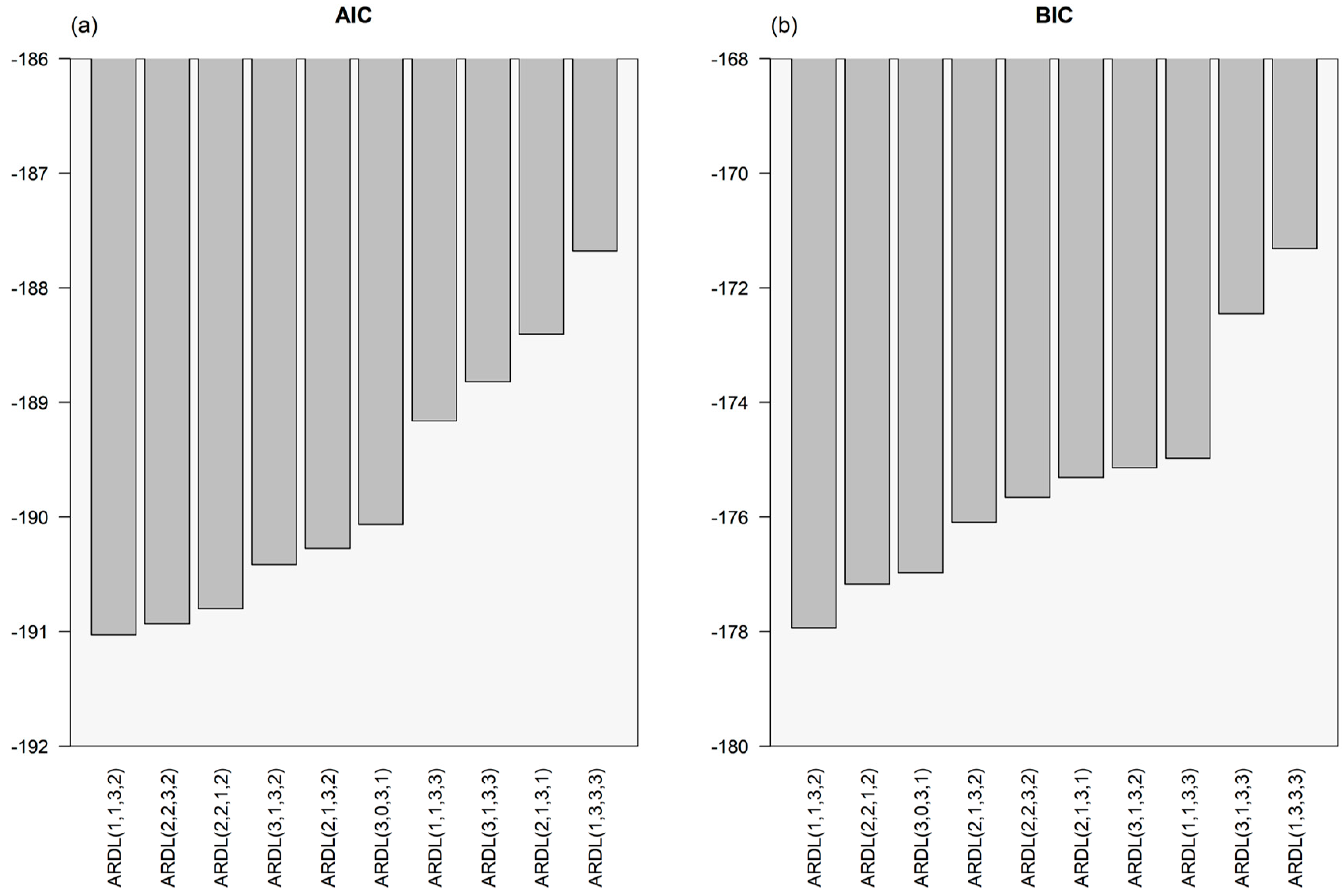
We determined the appropriate lags for the ARDL model based on a partial autocorrelation function (PACF) plot, Akaike Information Criterion (AIC), and BIC. Based on the PACF plot, several A R D L ( p ,   q 1 ,   ,   q k ) models with a maximum lag of 3 [45] were compared. The model with the lowest AIC and BIC was chosen as the best model. Figure 4 below shows ten A R D L ( p ,   q 1 ,   ,   q k ) models with their AIC and BIC values.
Based on Figure 4, ARDL(1,1,3,2) has the smallest AIC and BIC values. We chose ARDL(1,1,3,2) for our analysis throughout this paper.

4.2. Analysis of ARDL Bounds Cointegration Test

Based on the model diagnostic checking above, ARDL(1,1,3,2) can be used to model the long-run relationship between variables. The ARDL bounds cointegration test on ARDL(1,1,3,2) was conducted based on [51]. This approach uses the F-statistic to determine the existence of a long-run relationship between life expectancy as the dependent variable and health expenditure, GDP, and CO2 emissions as the independent variables. The summary of the ARDL bounds cointegration test is shown with critical values for k + 1 = 4 variables [51] in Table 3.
Table 3 shows that the F-statistic is 3.2986, which is greater than the upper bound critical value at a 10% significance level. Therefore, we reject the null hypothesis of no cointegration at a 10% level of significance. This finding confirms that there is evidence of cointegration between life expectancy, health expenditure, GDP, and CO2 emissions.

4.3. Result of Long-Run and Short-Run Relationships

Since the ARDL bounds cointegration test confirms the cointegration between variables, we can determine the long-run equation between the dependent variable and independent variables. Based on Equation (5), the estimated long-run coefficients are presented in Table 4. To obtain the short-run estimate and speed of adjustment, we estimated Equation (6) with the inclusion of ECT into the model. Short-run effects were captured by the coefficient of the first differenced variables [46]. The results of estimation using ordinary least square regression are shown in Table 5.
Based on Table 4, the results indicate that in the long run, the relationship between life expectancy and health expenditure is negative but statistically insignificant. Coefficient estimates of health expenditure indicate 1% increase in health expenditure will decrease life expectancy by 0.2229%. Furthermore, GDP and CO2 emissions have a positive but statistically insignificant relationship with life expectancy in the long run. Coefficient estimates for GDP and CO2 emissions indicate that a 1% increase in G D P and C O 2 will increase L E by 0.2613% and 0.0227%, respectively. This finding is supported by [37], which reported GDP has a positive but statistically insignificant relationship with life expectancy in Brazil. Reference [22] reported that in Malaysia, GDP has no direct impact on life expectancy; rather, it affects life expectancy through health resources and demographic variables. Reference [35] also reported similar findings where CO2 has a positive but statistically insignificant relationship with life expectancy, but it has a statistically significant positive relationship in the short run.
Based on Table 5, the results indicate that in the short run, a negative and statistically significant relationship was observed between health expenditure and life expectancy. A 1% increase in health expenditure will decrease life expectancy by 0.0404%. This means that an increase in health expenditure alone is insufficient to improve life expectancy, and it should be complemented with improvements from other aspects such as economic and socioeconomic well-being. Similar findings were recorded by [52], which reported a negative but statistically insignificant impact of health expenditure on life expectancy for developing countries. Public and private health expenditures have a statistically insignificant relationship with the life expectancy of the population. In a recent study [31], the under-five mortality rate in Malaysia has a statistically significant long-run relationship with out-of-pocket health expenditures rather than public and private health expenditures.
In the short run, there is a positive and statistically significant relationship between CO2 emissions and life expectancy. A 1% increase in CO2 emissions will increase life expectancy by 0.0346%. CO2 emissions are mainly the result of energy consumption and industrial processes. Higher CO2 emissions are a sign of positive economic activities which then translate to improved income and quality of life. CO2 emissions result from transportation and electricity generation, which is more prevalent in urban areas. Urbanization has more technological progress and healthcare facilities and hence can improve life expectancy [53]. However, the short-run relationship between GDP and life expectancy is statistically insignificant. A 1% increase in GDP will decrease life expectancy by 0.0041%. This is supported by [22], in which it is argued that there is no direct relationship between GDP and life expectancy. GDP affects life expectancy through health resources and demographic variables.
The error correction term, ECT, is negative and statistically significant which indicates the existence of cointegration. In addition, the speed of adjustment is represented by the coefficient of E C T t 1 , which is 17.26%, where any deviation from the long-run equilibrium between variables is corrected at 17.26% in the long run. The correction of the disequilibrium is 5.8 years, where 1 is divided by the coefficient of the ECT [54].
It is interesting to note that the findings indicate similar long-run and short-run relationships between CO2, health expenditure, and life expectancy. CO2 impacts life expectancy positively, which suggests that emerging economies such as Malaysia are still dependent on fossil fuel consumption, and it is also indicative of industrial and technological advancement. This factor results in positive economic development which can improve life expectancy. Reference [19] concluded that a positive relationship between CO2 and life expectancy resulted in an increase in health expenditure, which means more allocation is provided to ensure the population remains healthy, hence resulting in better healthcare service and longer life expectancy. The negative relationship between health expenditure and life expectancy can be explained by deteriorating health conditions that are caused by chronic diseases [55]. In Malaysia, reference [56] reported that the leading cause of death is due to cardiovascular diseases such as stroke and coronary heart disease. As aging and population growth continue to rise, a similar increasing trend in the incidence of cardiovascular diseases [57] results in an increase in health expenditure allocated to treatments and other medical procedures.
Although GDP has an inverse relationship with life expectancy in the short run, it positively impacts life expectancy in the long run. In the long run, a positive relationship between GDP and life expectancy implies that a better standard of living is driven by positive economic development. This condition encourages the population to employ and maintain a healthy lifestyle in terms of food, nutrition, and healthy behavior, which in turn extends their life expectancy [27]. In the short run, the negative relationship between GDP and life expectancy implies that positive economic development has an inverse effect on the health condition of the population. To encourage positive economic development, higher workforce productivity is required, which may affect the health status of the labor force. The inability to maintain a healthy lifestyle due to stricter work commitments can lead to health issues such as hypertension, which if left untreated can lead to fatal cardiovascular diseases. In Malaysia, reference [56] reported that 3 in 10 persons have hypertension or high blood pressure, and hypertension or high blood pressure is most likely to affect the older population.

4.4. Model Diagnostic

To check for the goodness of fit of the model, we conducted a diagnostic check on the ARDL(1,1,3,2) model. A serial correlation test, normality test, and heteroscedasticity test for the residuals were performed. Details of the diagnostic tests are summarized in Table 6.
From Table 6, it can be seen that our ARDL(1,1,3,2) fulfilled all the diagnostic requirements with an R-square of 0.9718, which indicates that 97.18% of deviation in the dependent variable is captured by independent variables. The model also shows an absence of autocorrelation and heteroscedasticity, while indicating that the residuals are normally distributed. The test statistic for the Durbin–Watson test for serial correlation is 2.0132, which indicates the absence of autocorrelation. The test statistic for the Jarque–Bera test is 0.80584, with a p-value of 0.6684. Therefore, we fail to reject the null hypothesis of normally distributed residuals. The test statistic for the Breusch–Pagan test is 15.961 with a p-value of 0.1008. Therefore, we fail to reject the null hypothesis of homoscedasticity, which means that the residuals are distributed with equal variance. Hence, the proposed model ARDL(1,1,3,2) is suitable for measuring the long-run and short-run relationship between life expectancy, health expenditure, economic development, and carbon emissions.

5. Conclusions

This study contributes to the existing literature by analyzing the long-run and short-run relationship between health expenditure, GDP, CO2 emissions, and life expectancy in Malaysia from 1997 to 2021. The ARDL bounds cointegration test confirmed the existence of a long-run relationship between the dependent (life expectancy) and independent variables (health expenditure, GDP, CO2 emissions). ARDL(1,1,3,2) was determined as the best model for the cointegration test based on the lowest values of AIC and BIC. All independent variables have a statistically insignificant relationship with life expectancy in the long run. GDP and CO2 emissions have positive effects on life expectancy, while health expenditure has negative effects on life expectancy. In the short run, all independent variables exhibit a statistically significant relationship with life expectancy, except for GDP. Health expenditure and GDP have negative effects on life expectancy, while CO2 emissions have positive effects on life expectancy. As argued by [22], GDP has no direct relationship with life expectancy; rather, it can affect life expectancy through health expenditure or other variables. The speed of adjustment indicates that the correction of any deviations from long-run equilibrium between variables is at 17.26% in the next period. Diagnostic tests on the ARDL(1,1,3,2) model indicate that the model shows an absence of autocorrelation and heteroscedasticity while indicating that the residuals are normally distributed.
The findings of this study are essential as they show that health resources and environmental factors affect life expectancy significantly in the short run. Therefore, greater attention should be given to these two factors, particularly in the short run, in ensuring that Malaysia can maintain the health and well-being of the nation in line with the Sustainable Development Goals. Based on the findings, effective policy recommendations can be made to ensure a sustainable relationship between life expectancy, CO2 emissions, GDP, and health expenditure. Since productivity and a healthy workforce are essential for economic growth, policies that can improve labor productivity while providing effective public health and environmental management are very important. Greater attention should be given to preventive measures and public awareness of morbidity and mortality due to chronic diseases, such as cardiovascular diseases, which are the leading cause of death in Malaysia [56]. Medical professionals can assist in increasing public awareness and shifting mindsets towards healthy aging, which is equally vital for improving public health and well-being. Moving forward, there is a need to focus on renewable energy by investing in research and development of technologies that have a low risk of environmental degradation.
Future research may extend the period of study to include years before 1997 and to compare long-run relationships of other countries. Although this study focused on the case of Malaysia, which may limit the generalization of the study, future research can extend and replicate the model used and compare it with other emerging economies. Nonetheless, this study contributes to the body of knowledge and is beneficial for academicians, practitioners, and policymakers in addressing the issue of the relationship between life expectancy, carbon emission, economic development, and healthcare expenditure faced by emerging and developing countries.

Author Contributions

Conceptualization, N.R. and R.R.; methodology, N.R. and R.R.; software, N.R.; formal analysis, N.R.; data curation, N.R.; writing—original draft preparation, N.R.; writing—review and editing, R.R.; visualization, N.R.; supervision, R.R. All authors have read and agreed to the published version of the manuscript.

Funding

This research received no external funding.

Institutional Review Board Statement

Not applicable.

Informed Consent Statement

Not applicable.

Data Availability Statement

The source of all data used in this study is reported in the reference list of this paper. They will be available upon request. These data were derived from the following resources available in the public domain: 1. Ministry of Health Malaysia, https://www.moh.gov.my/index.php/pages/view/58?mid=19 (accessed on 30 March 2023); 2. World Bank, https://data.worldbank.org/indicator/SP.DYN.LE00.IN, https://data.worldbank.org/indicator/EN.ATM.CO2E.KT (accessed on 26 July 2023); 3. Department of Statistics Malaysia, https://newss.statistics.gov.my (accessed on 6 July 2023).

Acknowledgments

Norkhairunnisa Redzwan would like to acknowledge the Ministry of Higher Education (MOHE) of Malaysia and Universiti Teknologi MARA (UiTM) for their support in her PhD studies at Universiti Kebangsaan Malaysia (UKM), under Skim Latihan Akademik Bumiputera (SLAB).

Conflicts of Interest

The authors declare no conflicts of interest.

References

  1. United Nations. World Population Ageing 2019; United Nations, Department of Economic and Social Affairs, Population Division: New York, NY, USA, 2019; ISBN 978-92-1-148326-0. [Google Scholar]
  2. Chen, Q.; Dietzenbacher, E.; Los, B. The Effects of Ageing and Urbanisation on China’s Future Rural and Urban Populations. Asian Popul. Stud. 2017, 13, 172–197. [Google Scholar] [CrossRef]
  3. Gu, D.; Andreev, K.; Dupre, M.E. Major Trends in Population Growth Around the World. China CDC Weekly 2021, 3, 604. [Google Scholar] [CrossRef]
  4. Cristea, M.; Noja, G.G.; Stefea, P.; Sala, A.L. The Impact of Population Aging and Public Health Support on EU Labor Markets. Int. J. Environ. Res. Public Health 2020, 17, 1439. [Google Scholar] [CrossRef]
  5. United Nations. World Urbanization Prospects 2018: Highlights; United Nations, Department of Economic and Social Affairs, Population Division: New York, NY, USA, 2019; ISBN 978-92-1-148318-5. [Google Scholar]
  6. Ahmed, Z.; Zafar, M.W.; Ali, S. Linking Urbanization, Human Capital, and the Ecological Footprint in G7 Countries: An Empirical Analysis. Sustain. Cities Soc. 2020, 55, 102064. [Google Scholar] [CrossRef]
  7. Sajid, M.R.; Muhammad, N.; Zakaria, R.; Bukhari, S.A.C. Modifiable Risk Factors and Overall Cardiovascular Mortality: Moderation of Urbanization. J. Public Health Res. 2020, 9, 410–416. [Google Scholar] [CrossRef]
  8. Bijari, N.B.; Mahdinia, M.H.; Mansouri Daneshvar, M.R. Investigation of the Urbanization Contribution to the COVID-19 Outbreak in Iran and the MECA Countries. Environ. Dev. Sustain. 2021, 23, 17964–17985. [Google Scholar] [CrossRef]
  9. Antai, D.; Moradi, T. Urban Area Disadvantage and Under-5 Mortality in Nigeria: The Effect of Rapid Urbanization. Environ. Health Perspect. 2010, 118, 877–883. [Google Scholar] [CrossRef]
  10. Liu, X.; Xu, Y.; Engel, B.A.; Sun, S.; Zhao, X.; Wu, P.; Wang, Y. The Impact of Urbanization and Aging on Food Security in Developing Countries: The View from Northwest China. J. Clean. Prod. 2021, 292, 126067. [Google Scholar] [CrossRef]
  11. Pena, M.S.B.; Bernabé-Ortiz, A.; Carrillo-Larco, R.M.; Sánchez, J.F.; Quispe, R.; Pillay, T.D.; Málaga, G.; Gilman, R.H.; Smeeth, L.; Miranda, J.J. Migration, Urbanisation and Mortality: 5-year Longitudinal Analysis of the PERU MIGRANT Study. J. Epidemiol. Community Health 2015, 69, 715–718. [Google Scholar] [CrossRef]
  12. Wicke, F.; Ernst, M.; Otten, D.; Werner, A.; Dreier, M.; Brähler, E.; Tibubos, A.; Reiner, I.; Michal, M.; Wiltink, J.; et al. The Association of Depression and All-Cause Mortality: Explanatory Factors and the Influence of Gender. J. Affect. Disord. 2022, 303, 315–322. [Google Scholar] [CrossRef]
  13. Walter, B.S.; DeWitte, S.N. Urban and Rural Mortality and Survival in Medieval England. Ann. Hum. Biol. 2017, 44, 338–348. [Google Scholar] [CrossRef]
  14. Warsame, A.A. Environmental Pollution and Life Expectancy in Somalia: Do Renewable Energy, Urbanization, and Economic Growth Matter? Environ. Sci. Pollut. Res. 2023, 30, 110528–110538. [Google Scholar] [CrossRef]
  15. Azam, M.; Uddin, I.; Saqib, N. The Determinants of Life Expectancy and Environmental Degradation in Pakistan: Evidence from ARDL Bounds Test Approach. Environ. Sci. Pollut. Res. 2023, 30, 2233–2246. [Google Scholar] [CrossRef]
  16. Georgescu, I.; Kinnunen, J. The Role of Foreign Direct Investments, Urbanization, Productivity, and Energy Consumption in Finland’s Carbon Emissions: An ARDL Approach. Environ. Sci. Pollut. Res. 2023, 30, 87685–87694. [Google Scholar] [CrossRef]
  17. Osei-Kusi, F.; Wu, C.; Tetteh, S.; Castillo, W.I.G. The Dynamics of Carbon Emissions, Energy, Income, and Life Expectancy: Regional Comparative Analysis. PLoS ONE 2024, 19, e0293451. [Google Scholar] [CrossRef]
  18. Rahman, M.M.; Rana, R.; Khanam, R. Determinants of Life Expectancy in Most Polluted Countries: Exploring the Effect of Environmental Degradation. PLoS ONE 2022, 17, e0262802. [Google Scholar] [CrossRef]
  19. Karma, E. Socioeconomic Determinants of Life Expectancy: Southeastern European Countries. Eur. J. Sustain. Dev. 2023, 12, 25. [Google Scholar] [CrossRef]
  20. Rjoub, H.; Odugbesan, J.A.; Adebayo, T.S.; Wong, W.-K. Investigating the Causal Relationships Among Carbon Emissions, Economic Growth, and Life Expectancy in Turkey: Evidence from Time and Frequency Domain Causality Techniques. Sustainability 2021, 13, 2924. [Google Scholar] [CrossRef]
  21. Osabohien, R.; Ayomitunde, A.T.; Bose, A.D.; Bose, J.L. Carbon Emissions and Life Expectancy in Nigeria. Int. J. Energy Econ. Policy 2021, 11, 497–501. [Google Scholar] [CrossRef]
  22. Chan, M.F.; Kamala Devi, M. Factors Affecting Life Expectancy: Evidence from 1980–2009 Data in Singapore, Malaysia, and Thailand. Asia Pac. J. Public Health 2015, 27, 136–146. [Google Scholar] [CrossRef]
  23. Department of Statistics Malaysia. Population Projections (Revised) Malaysia 2010–2040. Available online: https://newss.statistics.gov.my (accessed on 6 July 2023).
  24. World Bank. Life Expectancy at Birth, Total (Years). Available online: https://data.worldbank.org/indicator/SP.DYN.LE00.IN (accessed on 26 July 2023).
  25. Ling, C.H.; Ahmed, K.; Muhamad, R.; Shahbaz, M.; Loganathan, N. Testing the Social Cost of Rapid Economic Development in Malaysia: The Effect of Trade on Life Expectancy. Soc. Indic. Res. 2017, 130, 1005–1023. [Google Scholar] [CrossRef]
  26. Murthy, U.; Shaari, M.S.; Mariadas, P.A.; Abidin, N.Z. The Relationships between CO2 Emissions, Economic Growth and Life Expectancy. J. Asian Financ. Econ. Bus. 2021, 8, 801–808. [Google Scholar] [CrossRef]
  27. Wirayuda, A.A.B.; Chan, M.F. A Systematic Review of Sociodemographic, Macroeconomic, and Health Resources Factors on Life Expectancy. Asia Pac. J. Public Health 2021, 33, 335–356. [Google Scholar] [CrossRef]
  28. Jiang, J.; Luo, L.; Xu, P.; Wang, P. How Does Social Development Influence Life Expectancy? A Geographically Weighted Regression Analysis in China. Public Health 2018, 163, 95–104. [Google Scholar] [CrossRef]
  29. Ministry of Health. Malaysia National Health Accounts Health Expenditure Report 1997–2019; Ministry of Health Malaysia: Putrajaya, Malaysia, 2021.
  30. Bayati, M.; Akbarian, R.; Kavosi, Z. Determinants of Life Expectancy in Eastern Mediterranean Region: A Health Production Function. Int. J. Health Policy Manag. 2013, 1, 57. [Google Scholar] [CrossRef]
  31. Logarajan, R.D.; Nor, N.M.; Sirag, A.; Said, R.; Ibrahim, S. The Impact of Public, Private, and Out-Of-Pocket Health Expenditures On Under-Five Mortality in Malaysia. Healthcare 2022, 10, 589. [Google Scholar] [CrossRef]
  32. Nketiah-Amponsah, E. The Impact of Health Expenditures on Health Outcomes in Sub-Saharan Africa. J. Dev. Soc. 2019, 35, 134–152. [Google Scholar] [CrossRef]
  33. Shi, A. The Impact of Population Pressure on Global Carbon Dioxide Emissions, 1975–1996: Evidence from Pooled Cross-Country Data. Ecol. Econ. 2003, 44, 29–42. [Google Scholar] [CrossRef]
  34. Menz, T.; Welsch, H. Population Aging and Carbon Emissions in OECD Countries: Accounting for Life-Cycle and Cohort Effects. Energy Econ. 2012, 34, 842–849. [Google Scholar] [CrossRef]
  35. Ali, A.; Ahmad, K. The Impact of Socio-Economic Factors on Life Expectancy for Sultanate of Oman: An Empirical Analysis. Middle-East J. Sci. Res. 2014, 22, 218–224. [Google Scholar]
  36. Hill, T.D.; Jorgenson, A.K.; Ore, P.; Balistreri, K.S.; Clark, B. Air Quality and Life Expectancy in the United States: An Analysis of the Moderating Effect of Income Inequality. SSM-Popul. Health 2019, 7, 100346. [Google Scholar] [CrossRef] [PubMed]
  37. Duque, A.M.; Peixoto, M.V.; Lima, S.V.; Goes, M.A.O.; Santos, A.D.; Araújo, K.C.G.M.; Nunes, M.A.P. Analysis of the Relationship Between Life Expectancy and Social Determinants in a North-Eastern Region of Brazil, 2010–2017. Geospat. Health 2018, 13, 345–352. [Google Scholar] [CrossRef] [PubMed]
  38. He, L.; Li, N. The Linkages Between Life Expectancy and Economic Growth: Some New Evidence. Empir. Econ. 2020, 58, 2381–2402. [Google Scholar] [CrossRef]
  39. Angelov, I. The Square Theory of Economic Development. South Asian J. Soc. Stud. Econ. 2023, 18, 30–36. [Google Scholar] [CrossRef]
  40. Pelsa, I.; Balina, S. Development of Economic Theory–from Theories of Economic Growth and Economic Development to the Paradigm of Sustainable Development. DIEM Dubrov. Int. Econ. Meet. 2022, 7, 91–101. [Google Scholar] [CrossRef]
  41. Natsiopoulos, K.; Tzeremes, N.G. ARDL Bounds Test for Cointegration: Replicating the Pesaran et al. (2001) Results for the UK Earnings Equation using R. J. Appl. Econom. 2022, 37, 1079–1090. [Google Scholar] [CrossRef]
  42. R Core Team. R: A Language and Environment for Statistical Computing; R Foundation for Statistical Computing: Vienna, Austria, 2020; Available online: https://www.R-project.org/ (accessed on 2 November 2022).
  43. Ministry of Health. Malaysia National Health Accounts Health Expenditure Report 2011–2021; Ministry of Health Malaysia: Putrajaya, Malaysia, 2023.
  44. World Bank. CO2 emissions (kt)—Malaysia. Available online: https://data.worldbank.org/indicator/EN.ATM.CO2E.KT?end=2020&locations=MY&start=1997&view=chart (accessed on 26 July 2023).
  45. Gessesse, A.T.; He, G. Analysis of Carbon Dioxide Emissions, Energy Consumption, and Economic Growth in China. Agric. Econ. 2020, 66, 183–192. [Google Scholar] [CrossRef]
  46. Shaari, M.S.; Lee, W.C.; Ridzuan, A.R.; Lau, E.; Masnan, F. The Impacts of Energy Consumption by Sector and Foreign Direct Investment on CO2 Emissions in Malaysia. Sustainability 2022, 14, 16028. [Google Scholar] [CrossRef]
  47. Ghosh, S. The Impact of Economic Uncertainty and Financial Stress on Consumer Confidence: The Case of Japan. J. Asian Bus. Econ. Stud. 2022, 29, 50–65. [Google Scholar] [CrossRef]
  48. Narayan, P.K. The Saving and Investment Nexus for China: Evidence from Cointegration Test. Appl. Econ. 2005, 37, 1979–1990. [Google Scholar] [CrossRef]
  49. Phillips, P.C.; Perron, P. Testing for a Unit Root in Time Series Regression. Biometrika 1988, 75, 335–346. [Google Scholar] [CrossRef]
  50. Kwiatkowski, D.; Phillips, P.C.B.; Schmidt, P.; Shin, Y. Testing the Null Hypothesis of Stationarity Against the Alternative of a Unit Root: How Sure are We that Economic Time Series have a Unit Root? J. Econom. 1992, 54, 159–178. [Google Scholar] [CrossRef]
  51. Pesaran, M.H.; Shin, Y.; Smith, R.J. Bounds Testing Approaches to the Analysis of Level Relationships. J. Appl. Econom. 2001, 16, 289–326. [Google Scholar] [CrossRef]
  52. Kabir, M. Determinants of Life Expectancy in Developing Countries. J. Dev. Areas 2008, 41, 185–204. [Google Scholar] [CrossRef]
  53. Zhang, M.; Yang, Z.; Liu, L.; Zhou, D. Impact of Renewable Energy Investment on Carbon Emissions in China-An empirical study using a Nonparametric Additive Regression Model. Sci. Total Environ. 2021, 785, 147109. [Google Scholar] [CrossRef] [PubMed]
  54. Udemba, E.N.; Philip, L.D. Policy Insight from Renewable Energy, Foreign Direct Investment (FDI), and Urbanization Towards Climate Goal: Insight from Indonesia. Environ. Sci. Pollut. Res. 2022, 29, 54492–54506. [Google Scholar] [CrossRef] [PubMed]
  55. Ismail, Z.; Ahmad, W.I.W.; Hamjah, S.H.; Astina, I.K. The Impact of Population Ageing: A Review. Iran. J. Public Health 2021, 50, 2451. [Google Scholar] [CrossRef]
  56. Institute for Public Health. National Health and Morbidity Survey (NHMS) 2019: Non-Communicable Diseases, Healthcare Demand, and Health Literacy—Key Findings; Ministry of Health Malaysia: Putrajaya, Malaysia, 2020; ISBN 978-983-99320-6-5.
  57. Moran, A.; Gu, D.; Zhao, D.; Coxson, P.; Wang, Y.C.; Chen, C.-S.; Liu, J.; Cheng, J.; Bibbins-Domingo, K.; Shen, Y.-M.; et al. Future Cardiovascular Disease in China: Markov Model and Risk Factor Scenario Projections from the Coronary Heart Disease Policy Model–China. Circ. Cardiovasc. Qual. Outcomes 2010, 3, 243–252. [Google Scholar] [CrossRef]
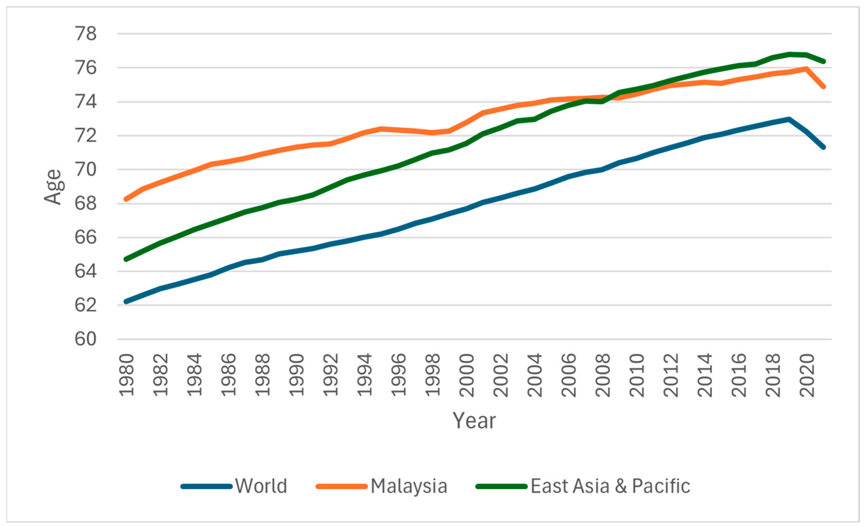
Figure 1. Historical trend of life expectancy (authors’ own construction based on data from [24]).
World 05 00030 g001
Figure 2. Framework for this study on effects of urbanization on life expectancy, proxied by health resources, environment, and economic development (based on authors’ model construction from literature).
World 05 00030 g002
Figure 3. Historical trend of variables: (a) life expectancy; (b) health expenditure per capita; (c) GDP per capita; (d) carbon dioxide emission per capita.
World 05 00030 g003
Figure 4. Plots of (a) AIC and (b) BIC for A R D L ( p ,   q 1 ,   ,   q k ) models.
World 05 00030 g004
Table 1. Description of variables.
VariableProxyUnitSources
Health resourcesTotal health expenditure per capitaRM[29,43]
EnvironmentCO2 emissions per capitaTonnes[24,44]
Economic developmentGDP per capitaRM[29,43]
Life expectancyLife expectancy at birthYear[24,44]
Table 2. Unit root test results.
VariablesPP Test StatisticsKPSS Test Statistics
LevelFirst DifferenceLevelFirst Difference
LE−2.44−16.9 **0.85504 ***0.32846
HE−0.267−25.9 ***0.9298 ***0.18128
GDP−0.469−27.1 ***0.91447 ***0.18215
CO2−2.71−25.6 ***0.79232 ***0.0386
** 5% level of significance; *** 1% level of significance.
Table 3. ARDL bounds cointegration test on ARDL(1,1,3,2).
F-Statistic:3.2986 *
Critical value boundsSignificance (%)Lower BoundUpper Bound
102.373.2 *
52.793.67
13.654.66
* 10% level of significance.
Table 4. Estimated long-run coefficients for ARDL(1,1,3,2).
VariableCoefficientStandard Errort-Statisticsp-Values
Constant3.1911361.91771.6640.1243
HE−0.222970.4947−0.45070.6609
GDP0.261320.52470.49810.6282
CO20.02270.11260.20180.8438
Table 5. Estimated short-run coefficients for ARDL(1,1,3,2).
VariableCoefficientStandard Errort-Statisticsp-Values
H E t −0.04041760.0111−3.6340.002449 ***
G D P t −0.00406920.0103−0.3950.698345
G D P t 1 −0.00037350.0127−0.0290.977004
G D P t 2 −0.03160400.0096−3.2880.004983 ***
C O 2 t 0.03458070.01172.9670.009596 ***
C O 2 t 1 −0.02284320.0137−1.6690.115862
E C T t 1 −0.17256840.0363−4.7420.000262 ***
*** 1% level of significance.
Table 6. Diagnostic test results.
TestResult (p-Value)
Durbin–Watson2.0132
Jarque–Bera0.80584 (0.6684)
Breusch–Pagan15.961 (0.1008)
R-square0.9718
Disclaimer/Publisher’s Note: The statements, opinions and data contained in all publications are solely those of the individual author(s) and contributor(s) and not of MDPI and/or the editor(s). MDPI and/or the editor(s) disclaim responsibility for any injury to people or property resulting from any ideas, methods, instructions or products referred to in the content.