Modeling the Impact of Global Warming on Ecosystem Dynamics: A Compartmental Approach to Sustainability

Abstract

Environmental degradation driven by human activities has heightened the need for sustainable development strategies that balance economic growth with ecological preservation. This study uses a compartmental model approach to examine the effects of global warming on ecosystem dynamics, focusing on how rising temperatures alter interactions across trophic levels. Three case studies of varying complexity, including a human ecosystem incorporating social and economic factors, were analyzed by integrating feedback loops between greenhouse gas emissions, temperature anomalies, and ecosystem responses. The results quantitatively demonstrate that even minor disruptions in one part of an ecosystem can cause significant instability across trophic levels, potentially driving the system to collapse in a short period. These findings from all case studies highlight the cascading impacts of global warming, underscoring the intricate relationship between climate change and ecosystem stability. Furthermore, this study offers qualitative insights into the potential consequences of climate change on biodiversity and resource availability in real ecosystems, highlighting the vulnerability of such systems and the importance of incorporating feedback mechanisms into environmental policy and decision-making processes. The approach employed in this study offers a more robust framework for understanding ecosystem responses and for developing strategies to enhance resilience against climate change, thereby protecting the long-term sustainability of ecosystems.

1. Introduction

There is growing recognition between both society and governments of the profound environmental damage resulting from human activities, particularly those driven by economic growth. The relentless exploitation of natural resources for industrial and commercial purposes is increasingly being seen as unsustainable, as the Earth’s finite resources are incapable of sustaining the ever-increasing demands of a global population [1,2].

Since the Industrial Revolution, global warming has been exacerbated by the excessive emissions of anthropogenic greenhouse gases (GHG). These changes in abiotic factors, such as solar radiation, temperature, and rainfall, directly affect biotic factors, limiting their natural development and functioning. This has led to anomalies and chains of catastrophes globally, including polar ice melt and sea level rise [3,4], which result in floods [5], droughts [6], forest and agrarian disturbances [7,8], and wildfires [9], potentially leading to species extinction [10]. Thus, it is evident that this issue must be addressed from a sustainability perspective, which entails the comprehensive analysis and integration of various ecological, social, and economic concepts through a multidisciplinary approach [11].

This approach requires the formulation of public policies that account not only for ecological but also socioeconomic factors, targeting inefficiencies in carbon emission management and resource consumption. Recent studies underscore the potential of infrastructural advancements, such as the implementation of high-speed rail systems, to enhance urban carbon efficiency by optimizing transportation networks and reducing emissions [12]. Furthermore, economic interventions like tax policy reforms have been shown to impact carbon emission efficiency across industries, demonstrating the critical role of policy in managing carbon emissions [13].

These insights align with growing evidence that socioeconomic strategies are essential for addressing environmental challenges. For instance, research has demonstrated that circular economy models, which prioritize resource reuse and minimize waste, significantly contribute to both economic resilience and environmental sustainability [14]. Additionally, the implementation of green financial policies, such as carbon pricing mechanisms and sustainable investment incentives, has proven effective not only in mitigating environmental degradation but also in fostering economic growth [15]. Equally critical is the need to strike a balance between enhancing agricultural productivity and conserving ecosystems [16].

Studying ecosystems from a sustainability perspective enables us to comprehend how these systems can be utilized while preserving global balance [17]. However, sustainability analysis requires multidisciplinary studies, which are subject to certain limitations, such as the incompatibility of information due to its diverse nature, challenges in integrating data from various sources, and differing methodologies across disciplines [18,19]. These limitations can hinder the development of comprehensive and actionable insights; therefore, it is necessary to employ appropriate tools to manage this data diversity [20]. In this sense, mathematical models allow for the precise and concrete representation of ecosystems, enabling the manipulation of system variables to understand their behavior and stability [21]. Mathematical models have been employed for various purposes and applications; for instance, to predict the impact of climate change on biodiversity [22], optimize resource management [23], and assess the resilience of ecosystems [24].

Despite these models being typically developed for particular ecological systems, several models have been created to better understand and manage human impacts on a global scale. For instance, Integrated Assessment Models (IAMs) combine data from various disciplines to evaluate the environmental, economic, and social impacts of different policy scenarios [25,26]. Ecosystem models, such as the Integrated Model to Assess the Global Environment (IMAGE), the Global Change Assessment Model (GCAM), and recently, the HARMONEY model, provide insights into how human activities affect biodiversity, ecosystem services, and climate change [27,28,29].

However, these models often require extensive data and can be computationally complex. In this regard, compartmental models are a valuable type of mathematical model for representing complex systems by simplifying them into interconnected compartments. These compartments represent conceptual states or categories within the system, grouping certain system elements of interest based on key characteristics. The interactions between compartments, which represent flows of matter, energy, and/or information, are typically described using differential equations [30]. While compartmental models have clear limitations, such as the need for simplifying assumptions about the system being modeled and the potential for uncertainty in parameter estimation, they remain powerful tools for understanding and analyzing a wide range of systems in diverse fields of study.

The advantages of compartmental models include their ability to capture the essential dynamics of complex systems in a relatively simple and interpretable framework, making them valuable tools for hypothesis testing, scenario analysis, and policy evaluation. For instance, compartmental models have been extensively used during the COVID-19 pandemic to predict the impact of vaccination strategies and to optimize public health responses [31,32,33]. Compartmental models are also widely used in ecological modeling to assess the sustainability and resilience of ecosystems. This approach aids in understanding the intricate direct and indirect correlations among ecosystem components and how they respond to various disturbances and stressors by providing a detailed representation of their dynamics [34]. This predictive capability is crucial for managing natural resources, making this approach a powerful tool in both theoretical explorations and practical decision-making. It supports the formulation of strategies and robust environmental policies that protect biodiversity and mitigate the impacts of human activity, ensuring that interventions are both effective and scientifically grounded [35,36].

Despite its wide applications and significant utility, the mathematical modeling of human ecosystems still presents several challenges. For instance, long-term analyses must account for the complex feedback mechanisms intrinsic to natural systems. These mechanisms can provide ecosystems with either greater or lower resilience than initially expected. Feedback loops are critical to understanding the dynamics of complex systems and are essential for accurately modeling ecosystem behavior under external stress. These interactions can lead to nonlinear dynamics and tipping points that are difficult to predict without proper consideration. Neglecting these dynamics could result in significant inaccuracies in the conclusions drawn [11].

In recent years, feedback loops have become a focal point in the mathematical modeling of global warming. These loops capture the complex interactions between different elements of ecosystems, such as GHG emissions, temperature anomalies, and their cascading effects on biodiversity and resource availability. For instance, Jones et al. [37] and Schuur et al. [38] demonstrated that positive feedback loops, such as those triggered by permafrost thaw, could lead to a much faster and more severe intensification of global warming than previously predicted. Moreover, Kimmins et al. [39] and Martin and Schlüter [40] introduced hybrid models combining deterministic and data-driven approaches, which have enhanced our ability to simulate the scaling of local disturbances into global impacts. Dong and Huang [41] and Ripple et al. [42] provided critical insights into human-driven feedback loops, which exacerbate environmental degradation, showing that human activities significantly amplify the impacts of global warming beyond natural processes. Additionally, global warming has affected the phenology of a wide range of species being a driver of ecosystem instability [43]. Janni et al. [44] and Zandalinas et al. [45] have shown that rising temperatures disrupt plant growth, leading to declines in primary producers. This reduction at the base of the food web triggers trophic cascades throughout the ecosystem, as observed by Schmitz et al. [46] and Gonzalez et al. [47]. These relevant advances highlight the critical importance of incorporating dynamic feedback loops into ecosystem models, especially when assessing the long-term impacts of climate change on sustainability.

Therefore, this present study builds upon these advances by incorporating dynamic feedback loops into ecosystem models, particularly focusing on the indirect effects of global warming on trophic interactions, based on the compartmental model proposed by Rodriguez-González et al. [34]. Before the integrated model, the approach was initially applied in two smaller and simpler models from the literature to lay the groundwork for the current comprehensive analysis. The enhanced models incorporate equations that describe the relationship between GHG emissions and temperature increases and their impact on vegetative development and human mortality rates, which are critical driving forces in the model.

This paper integrates both qualitative and quantitative aspects to analyze the impact of global warming on ecosystem dynamics. The qualitative aspect focuses on the conceptual understanding of feedback loops, ecosystem tipping points, and species-specific responses to climate change, drawing from the extensive literature to provide a descriptive analysis of how global warming affects ecosystem structure and function. The quantitative aspect, on the other hand, relies on mathematical models to simulate these effects and generate predictions about future changes in ecosystems. These models include compartmental representations of GHG emissions, temperature anomalies, and their impacts on vegetation and human mortality, providing a detailed quantitative analysis of the complex interactions within ecosystems. This approach provides a comprehensive understanding of the interactions between global warming and ecosystem dynamics.

2. Materials and Methods

The models used as case studies are constructed under a predator–prey approach, which has been widely applied to simulate complex biological food webs [48] and to analyze the stability of ecosystems [49]. This approach has also proven particularly useful in examining human ecosystems impacted by various stressors, including social inequity [34], the inclusion of biofuels in the trophic chain [50], increased consumption rates [51], population explosion [21], and water stress [36]. Figure 1 shows a generalized predator–prey compartmental model, which comprises two level species: predator (green) and prey (blue). The dynamics of the compartments are described by a set of differential equations, the general form of the Lotka–Volterra for a multi predator–prey system defined in Equation (1). This equation is constructed through mass balance, incorporating terms involving compartment natality and subtracting terms involving mortality.

$${\displaystyle \frac{d{Y}_i}{dt}}=\alpha Y_i+\left(\sum _{j\ne i}{\gamma }_{ij}{Y}_i{Y}_j\right)-\mu Y_i$$

(1)

where $d{Y}_i/dt$ is the change of compartment $i$ over time, $Y_i$is the current value of the compartment $i$, and $\alpha$ y $\mu$ are the compartment i birth and death rates due to natural causes, respectively. Meanwhile, ${\gamma }_{ij}$ represents the birth/mortality rate due to consumption, being positive when compartment i acts as a predator and negative when it acts as prey; $Y_j$ denotes the compartment with which it interacts.

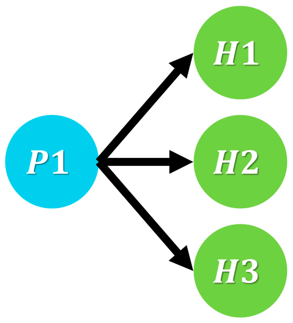
2.1. Basic Multi Predator–Prey Model

The first case study is derived from Chapra and Canale [52]. The model is graphically represented in Figure 2, which consists of four compartments distributed across two trophic levels: a plant (P1) serves as prey, and three herbivores (H1, H2, and H3) act as predators.

2.2. Multi-Level Predator–Prey Model

The second case study is based on the work of Pawlowski et al. [53] and is graphically represented in Figure 3. This model is structured trophically and comprises a pool of abiotic resources (RP), three different types of plants (P1, P2, and P3), three herbivores (H1, H2, and H3), two types of carnivores (C1 and C2), and one omnivore (O1). Unlike the previous model, in this case study, compartments simultaneously serve as both prey and predator within a closed-mass system. Material balance is maintained through the reintegration of waste back into the nutrient pool (RP). In Figure 2, solid lines depict the flow of natural consumption between species, as typically seen in food chains within ecosystems, while semi-continuous lines represent the reincorporation of matter back into the ecosystem following the death or natural waste of the compartments.

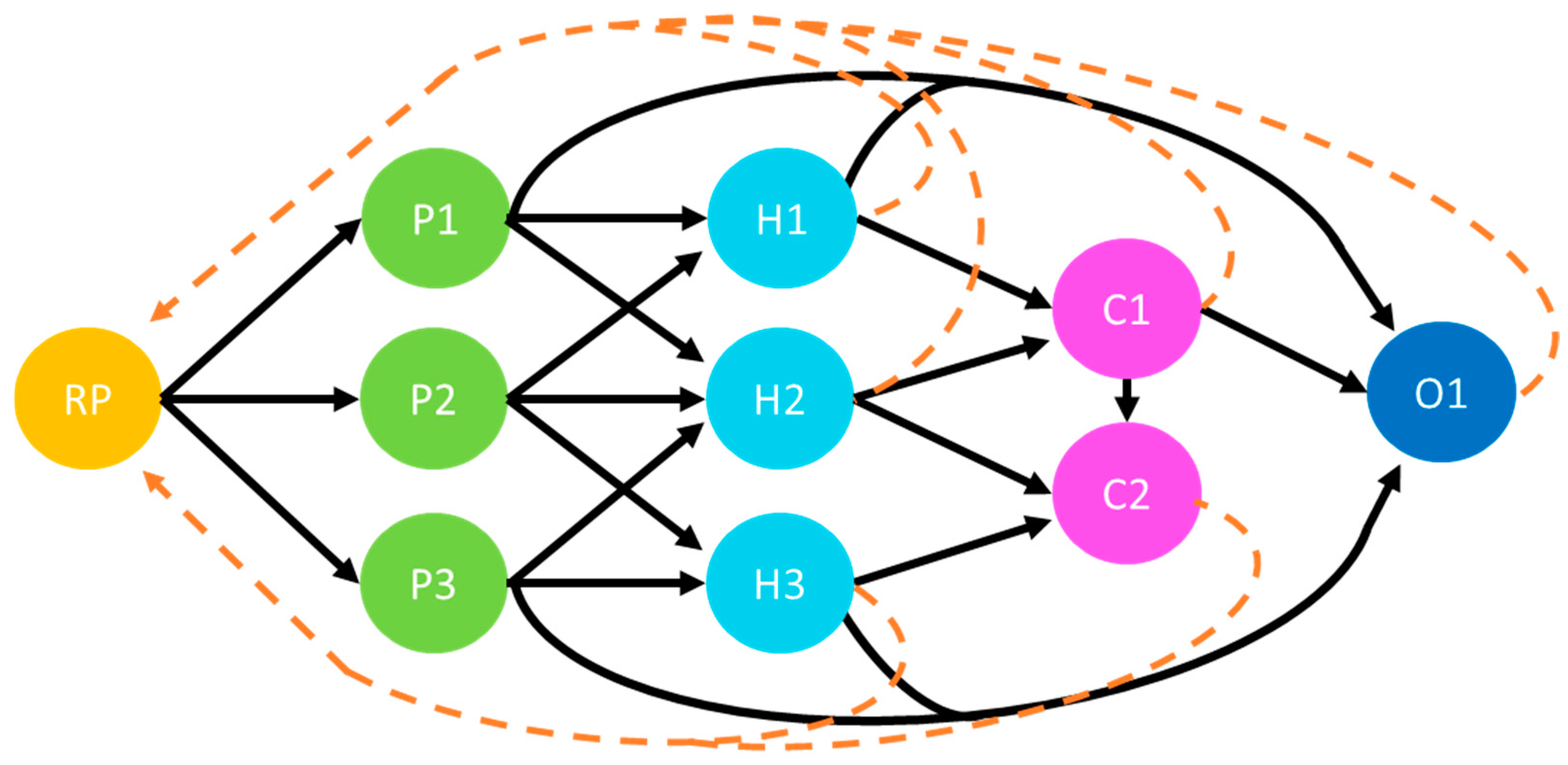
2.3. Generalized Sustainability Socio–Ecological Model (GSSEM)

The third case study takes as a basis the model presented by Rodriguez-Gonzalez et al. [34], which is graphically represented in Figure 4. The structure consists of 14 trophically organized compartments. In the biotic levels, there are two types of compartments: the domestic, which includes the agricultural sector (P1) and the livestock sector (H1), and the wild, which consists of compartments that either directly interact with humans, such as grasslands (P2), herbivores (H2), and carnivores (C1), with the latter two preying on the domestic compartments, or that do not directly interact with humans, such as plants (P3), herbivores (H3), and carnivores (C2). On the other hand, the abiotic level is represented by three resource pools: the primary pool, which supplies essential resources to the trophic chain (RP); the second pool, which represents waste disposal (IRP); and the third, which represents energy resources (ERP). Finally, the anthropic level includes human households (HH), the energy sector (EP), and the industrial and services sector (IS).

All compartments are interconnected by arrows, illustrating the dynamic relationships within the closed mass system. Solid lines represent the mass flow from natural consumption, semi-continuous lines denote human-controlled consumption, and dotted lines describe the flow of matter resulting from the death and waste of the compartments. Dot-dash lines define the flow of services, including industrial products and energy.

Although the model is based on the Lotka–Volterra trophic framework, it is refined by distinguishing between two main types of flows: natural and human-driven. The economic dimension comprises four compartments representing distinct productive sectors: agrarian (P1), livestock (H1), industrial and services (IS), and energy (EP). Meanwhile, the social dimension is associated with the household compartment (HH), which consumes resources from all productive sectors, such as food, energy, and manufactured goods. Both the economic and social dimensions contribute to greenhouse gas (GHG) emissions, with emissions directly linked to the levels of activity in their respective compartments. Changes in these levels affect the system’s overall carbon footprint, thus linking human-driven activities to environmental degradation and completing the global warming feedback loop.

Given that the model developed by Rodriguez-Gonzalez et al. [34] serves as the foundation for this case study, this section outlines the essential elements that define the integrated ecological, economic, and social dynamics. For comprehensive details of the model’s structure and assumptions, please refer to the original work [34].

In the natural compartments, mass flows retain the original Lotka–Volterra form (Equation (1)), characterized by a bilinear product term for interactions between compartments and a linear term for natural growth and mortality [54,55]. However, in the productive sectors, flows are not driven by the biotic levels of the compartments but instead depend on human needs, which are modeled by algebraic equations.

Initially, the per capita wage (W) serves as an indicator of the system’s economic health and is determined by an economic function that considers labor availability and the supply–demand gap in the industrial and services sector (IS), which impacts production and consumption rates. Subsequently, the economic sectors (P1, H1, IS, and EP) adjust pricing and production based on supply–demand imbalances, while their demand is calculated considering the inter-sector competition, with variables influenced by sector-specific prices and aggregated demands. Additionally, the population dynamic is modeled with growth and mortality terms, including a health-related factor that considers the effects of chronic degenerative diseases driven by nutrition disparities. Finally, the model estimates the atmospheric GHG concentration in carbon monoxide equivalents ($C{O_2}_{eq}$) by assessing emissions per compartment at each time step, factoring in emissions from human sectors and mitigation by natural compartments. This step allows the model to trace the system’s net impact on atmospheric $C{O_2}_{eq}$ over time.

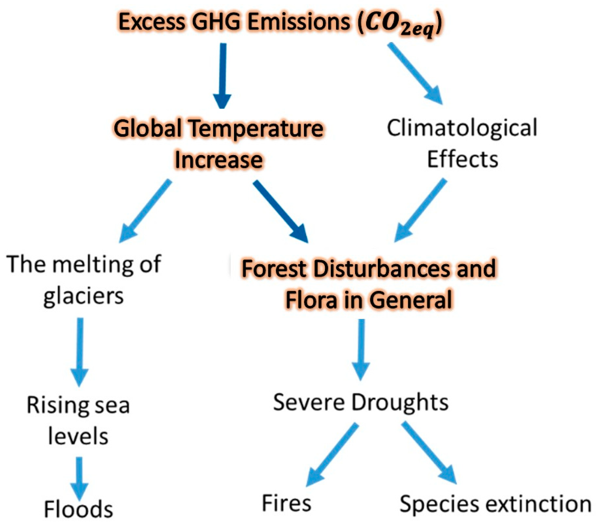
2.4. Global Warming Approach

Excessive GHG emissions trigger a cascade of environmental changes on Earth (Intergovernmental Panel on Climate Change [56]. Some of the primary direct effects include rising global temperatures and altered climatological patterns, which, in turn, precipitate a series of indirect consequences, such as floods, wildfires, and species extinctions, as illustrated in Figure 5 [57,58]. While the impacts of global warming are multifaceted and involve a wide range of environmental changes, this study focuses primarily on temperature anomalies as the key driver. These anomalies directly influence plant growth rates, which form the foundational biotic level of ecosystems, being the only indirect effect explicitly addressed. Any disruption in plant growth is likely to cascade through trophic-level dynamics, affecting ecosystem stability and revealing the potential indirect impacts of climate change across all ecosystem elements, including, ultimately, GHG emissions. This interaction sets a feedback loop within the system, highlighting the broad and interconnected effects of global warming.

Figure 6 shows a schematic representation of the global warming feedback loop. Arrows indicate interactions between greenhouse gas emissions, atmospheric CO₂ concentration, temperature anomalies, and ecosystem responses. Compartments emit GHG according to their nature, leading to an increase in the atmospheric concentration of carbon dioxide equivalents. This elevation induces changes in global system temperature, which in turn significantly impacts the development and behavior of the system’s elements.

In that context, global temperature ($T$) is a dynamic variable determined by Equation (2), using a constant ideal temperature $T_{opt}$, which serves as the reference value, plus a term representing the temperature anomaly ($A_T$), which signifies a deviation from the reference value. A positive anomaly suggests that the temperature is warmer than the reference value, whereas a negative anomaly indicates cooler conditions [59].

$${\displaystyle \frac{dT}{dt}}=T_{opt}+A_T$$

(2)

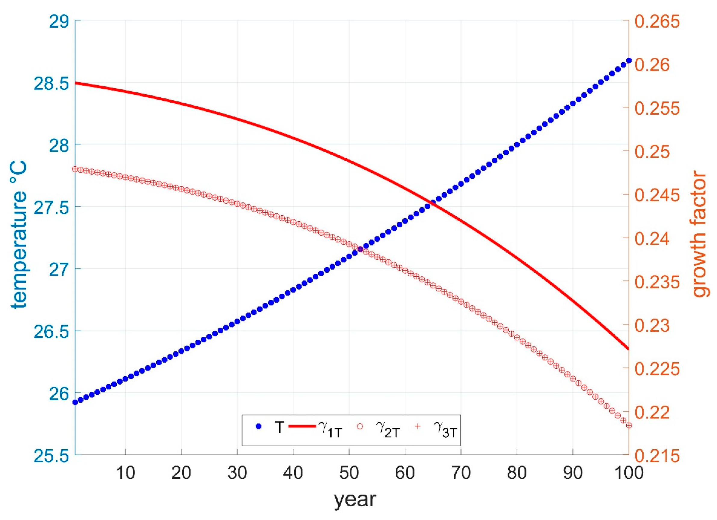
2.4.1. Global Temperature and Time

The first two case studies do not monitor the atmospheric concentration of GHG, as they do not encompass a global ecosystem. Consequently, to accurately represent temperature dynamics, global warming is modeled through an equation that varies with time ($t$). The translational movement of the planet significantly influences the variation of natural resources, altering temperatures according to seasonal changes throughout the year [36]. Given the oscillatory nature of predator–prey models, they mimic this natural variation, with each cycle in the model corresponding to one year. Utilizing historical data on the increase in global mean temperature anomalies ($A_T$) from recent decades, provided by the Goddard Institute for Space Studies [60], the time-function of the anomalies is fitted into Equation (3) as shown in Figure 7.

$$A_T=a{t}^2-bt-c$$

(3)

where $a$, $b$, and $c$ are constant parameters fitted to the cycle of each case study.

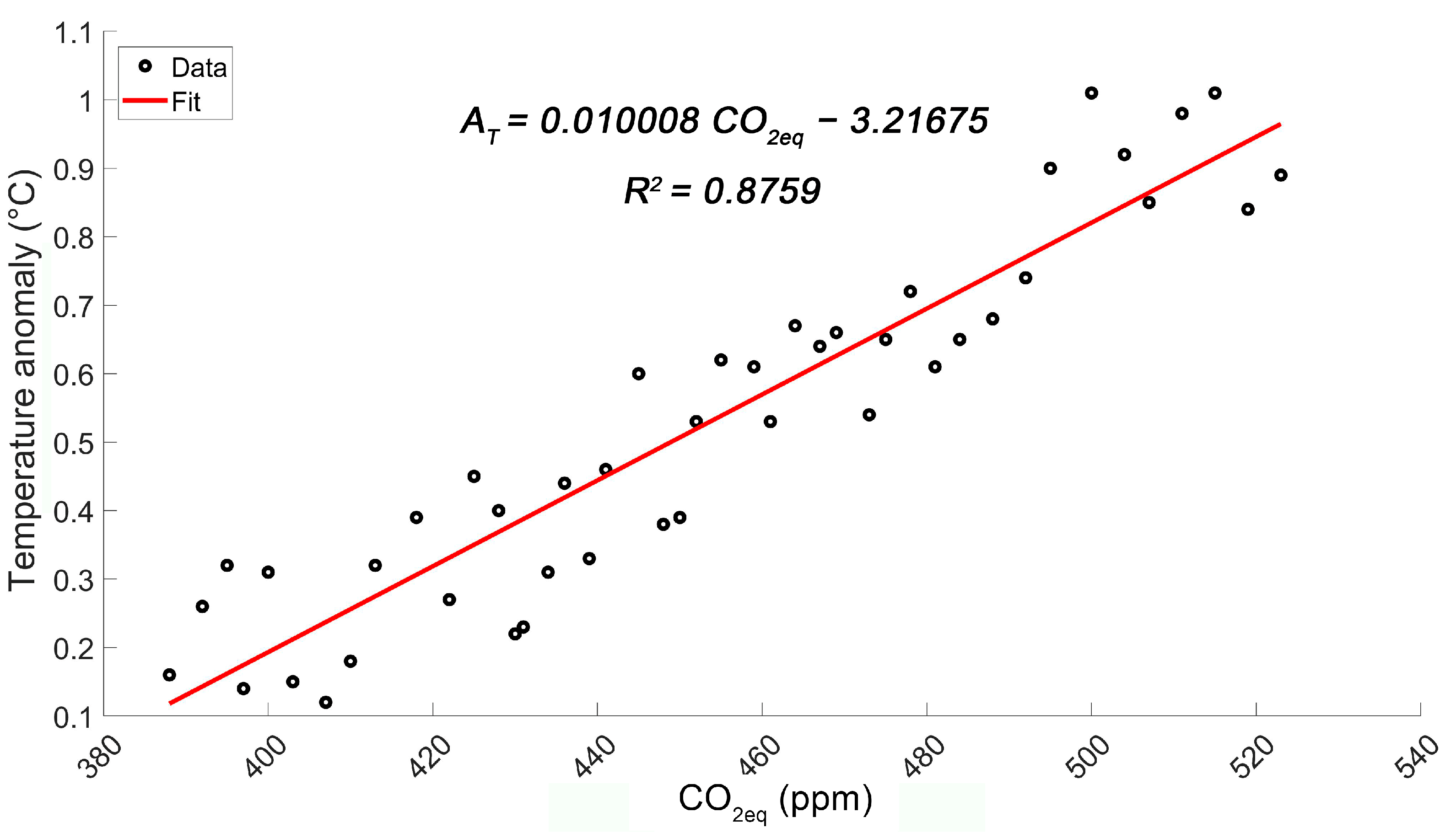
2.4.2. Global Temperature and GHG

As previously mentioned, the GSSEM does monitor the atmospheric concentration of GHG. It is well known that there is a correlation between this concentration and global temperature: higher levels of GHG in the atmosphere lead to higher global temperatures, while lower levels result in cooler temperatures. As Figure 8 shows, Equation (4) is derived by correlating the historical data on global mean temperature anomalies [60] with CO_2eq values provided by the NOAA [59]. This equation enables the prediction of temperature anomalies based on atmospheric CO₂eq concentrations for any given period.

$$A_T=0.010008C{O}_{2_{eq}}-3.21675$$

(4)

2.4.3. Global Temperature and Development

Temperature is a fundamental factor in plant growth. The maximum rate of plant development is achieved at an optimal temperature that varies depending on the characteristics of the plant. As the temperature deviates from this optimal point, the growth rate of the plant decreases. Significant deviations from this temperature can reach critical thresholds, potentially leading to a cessation of growth [61]. Recently, Paiva et al. [62] proposed modeling this change in plant growth rate as a symmetric single-peak Gaussian function of temperature. This approach was integrated into a Daisyworld model to describe the emission and absorption of GHG. Consequently, the constant value that describes the natural reproduction characteristics of the plant is replaced by the variable ${\gamma }_T$ calculated with Equation (5).

$${\gamma }_T=g{e}^{-{\displaystyle \frac{{(T-T_{opt})}^2}{s}}}$$

(5)

where$g$ is the base growth rate and s is the variance.

Photosynthesis operates most efficiently within a specific temperature range, generally recognized as 20 to 25 °C. Above this range, particularly when temperatures exceed 25 °C, respiratory activities tend to increase [63]. Therefore, the general optimal temperature ($T_{opt}$) is established at 25 °C. This temperature falls within the broader critical limits for plant survival, ranging from 0 °C to 50 °C [61,64]. Such a setting ensures that the temperature supports optimal photosynthetic activity while accommodating the physiological limits of the plants.

Finally, temperature not only affects biodiversity development; in the case of humans, the increase in deaths related to climate change is evident [65]. Therefore, to capture this temperature influence over mortality, a modification in the human death rate ${\mu }_T$ is also proposed as a symmetric single-peak Gaussian function. However, in this case, the function is inverted to represent an increase in the base value of the variable. In other words, at the optimal temperature, the death rate is the natural one, but as the temperature moves away from this point, the number of deaths increases due to various factors such as disease prevalence. Equation (6) shows this approach, where the linear term is added to shift the axis and position the optimal value at the base death rate value $m$, which is a function of time. Figure 9 illustrates the relationship between ${\gamma }_T$ (green) and ${\mu }_T$ (red) concerning the change of the base values (25 °C) of $g$ and $m$, respectively, following the Paiva et al. [62] approach. It is important to emphasize that the baseline death rate $m$ is a time-dependent function determined by Equation (7), which has been fitted using long-term historical data [34].

$${\mu }_T=-m_{\left(t\right)}{e}^{-{\displaystyle \frac{{\left(Temp-T_{opt}\right)}^2}{s}}}+2m_{\left(t\right)}$$

(6)

$$m_t=-0.0035\ast Ln\left(t\right)+0.020536$$

(7)

3. Results and Discussion

Three case studies of increasing complexity were modeled and simulated to analyze ecosystem responses to global warming impacts. Each case study represents a specific literature-based ecosystem configuration, which is then enhanced with the global warming approach outlined in the Methods section. This enhancement allows for observing both direct impacts on primary producers and indirect consequences on higher trophic levels. All models were coded in MATLAB and simulated over a 100-year period to capture the long-term effects of global warming on the systems. Initially, the models were run without integrating global warming to establish a baseline. In each model, the mass of the compartments is a conceptual representation of the combined mass of all involved species. These values are expressed in arbitrary units, referred to as mass units (mu), rather than in specific units of measurement.

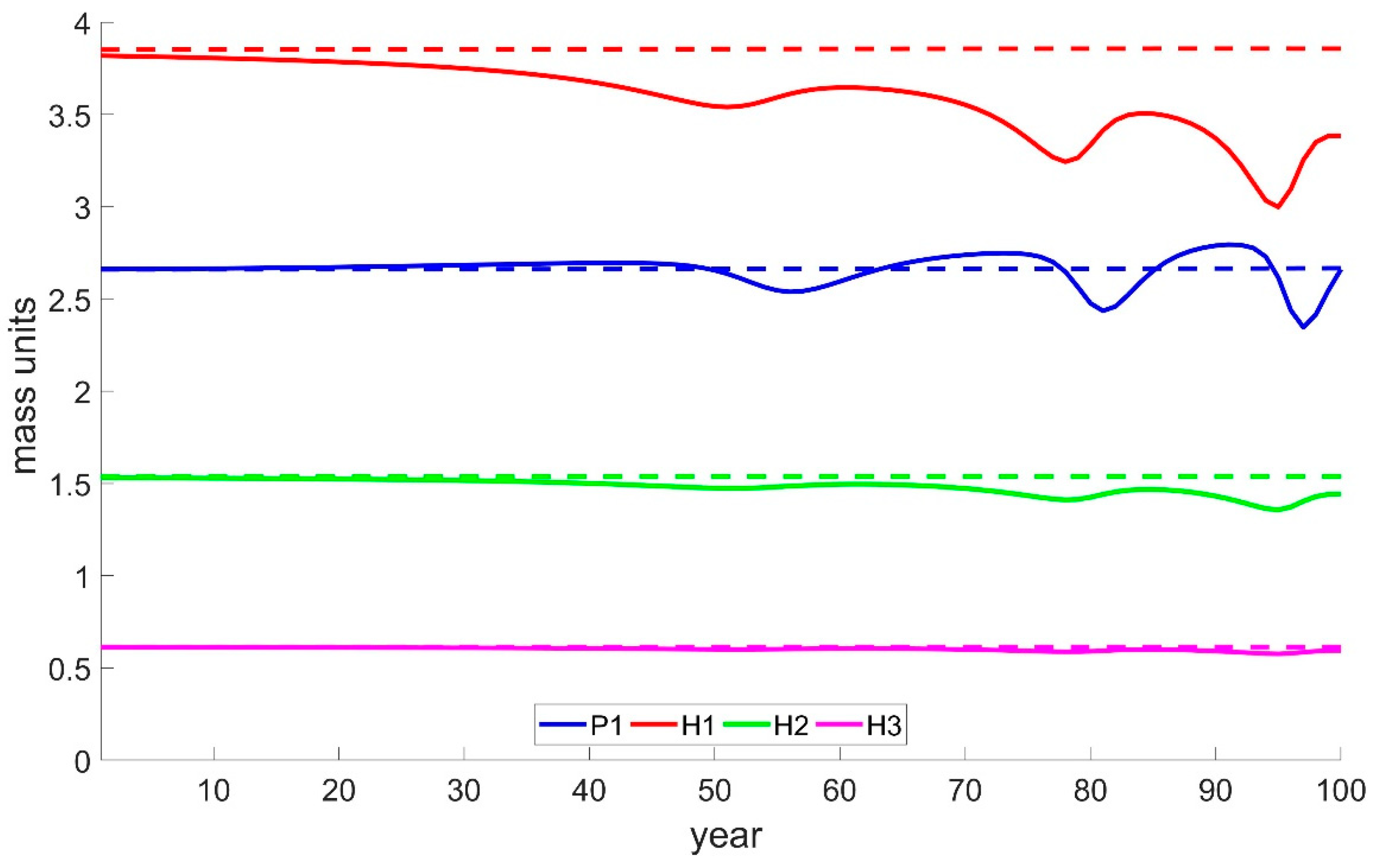
3.1. Case Study 1: Basic Multi Predator–Prey Model

The basic multi-predator–prey model was initially simulated for 20 time units (tu) to determine the period length. As shown in Figure 10, the model exhibits a repeating cycle every 9.5141 tu, indicating that this time in the model is equivalent to one year in the real world. Consequently, Equation (3) is transformed into Equation (8), with the year 2020 being considered the initial point in the simulation.

$$A_T=1.0045{ \times 10}^{-6}{t}^2-2.1364118{ \times 10}^{-3}t-0.8777995343$$

(8)

Once the model is complete, it is simulated using the initial values and parameters presented in

Table 1. Parameters and initial values for case study 1.

Growth Parameters						Initial Values
Plant		Herbivores
${\alpha }_{P1}$	1.2	${\mu }_{H1}$	0.20	${{\gamma }_2}_{P1H1}$	0.532	$P{1}_0$	2
${{\gamma }_1}_{P1H1}$	0.02	${\mu }_{H2}$	0.10	${{\gamma }_2}_{P1H2}$	0.266	$H{1}_0$	1.5
${{\gamma }_1}_{P1H2}$	0.02	${\mu }_{H3}$	0.05	${{\gamma }_2}_{P1H3}$	0.133	$H{2}_0$	1
${{\gamma }_1}_{P1H3}$	0.02					$H{3}_0$	0.5

Note: ${\alpha }_{P1}$ is the birth rate of the plant compartment P1; ${\gamma }_{1_{P1Hi}}$ is the plant P1 death factor due to being consumed by herbivore Hi; ${\gamma }_{2_{P1Hi}}$ is the herbivore Hi growth factor due to consumption of plant P1; finally, ${\mu }_{Hi}$ is the herbivore Hi death rate.

. Figure 11 illustrates the temperature profile in blue, which increases by almost 3 °C over the simulation period. This temperature rise significantly influences the plant growth factor, depicted in red in the same figure, causing a rapid and continuous decline. By the end of the simulation period, this factor decreases by 12%, from an initial value of 1.19 to 1.04. This decline underscores the sensitivity of primary producers to even modest temperature increases, as their growth rates are often closely linked to optimal thermal conditions [8], emphasizing the importance of stable thermal conditions for supporting ecosystem resilience.

This performance leads the system to gradual instability, as illustrated in Figure 12. The figure displays the mass profiles of the compartments over the simulated period, with the x-axis representing time in years and the y-axis showing mass. Solid lines indicate the case study results, while dashed lines represent the baseline conditions. In the short term, the system appears to maintain stability; however, as the simulation progresses, a clear trend of accelerated decline in the herbivore populations emerges, particularly evident in the middle to the latter half of the period. On the other hand, while the P1 compartment does not show a significant decrease in mass, its variability increases markedly over time, indicating growing fluctuations that signal impending instability in the system. These findings align with recent projections by Nahar et al. [61], which demonstrated that temperature-induced changes in plant metabolism could lead to significant shifts in primary productivity. This outcome also corroborates previous studies showing that primary producer losses trigger declines across trophic levels, as observed by Estes et al. [66] in real-world ecosystems.

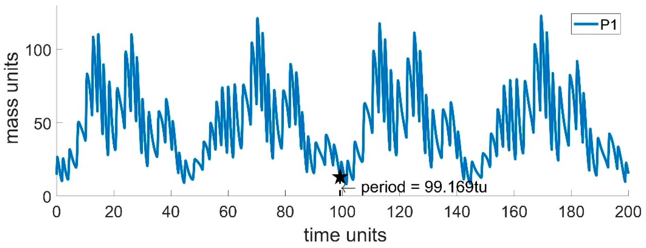
3.2. Case Study 2: Basic Multi Predator–Prey Model

The multi-level predator–prey model was initially simulated for 200 tu to determine the period length. Since the model comprises different elements with very varying periods, P1 is used as the reference point due to its having the longest period. As shown in Figure 13, the model exhibits a repeating cycle every 99.169 tu, indicating that this time in the model is equivalent to one year in the real world. Given this correspondence, and with the year 2020 set as the starting point for the simulation, Equation (3) is subsequently transformed into Equation (9). The initial values as well as growth parameters are described in

Table 2. Parameters and initial values for case study 2.

Growth Parameters						Initial Values
Plant		Herbivores		Carnivores/Omnivore		${RP}_0$	7.93
${\gamma }_{P1H1}$	0.01	${\gamma }_{H1C1}$	0.01	14.59	0.01	$P{1}_0$	14.59
${\gamma }_{P1H2}$	0.01	${\gamma }_{H1O1}$	0.01	${\gamma }_{C1O1}$	0.01	$P{2}_0$	32.89
${\gamma }_{P1H3}$	0.01	${\gamma }_{H1RP}$	0.1	${\gamma }_{C1RP}$	0.1	$P{3}_0$	13.76
${\gamma }_{P2H1}$	0.01	${\gamma }_{H2C1}$	0.01	${\gamma }_{C2RP}$	0.75	${H1}_0$	9.16
${\gamma }_{P2H2}$	0.01	${\gamma }_{H2C2}$	0.01	Resources		${H2}_0$	37.5
${\gamma }_{P2H3}$	0.01	${\gamma }_{H2RP}$	0.1	${\gamma }_{O1RP}$	0.75	${H3}_0$	11.47
${\gamma }_{P3H1}$	0.01	${\gamma }_{H3C1}$	0.01	${\gamma }_{RPP1}$	0.25	${C1}_0$	26.03
${\gamma }_{P3H2}$	0.01	${\gamma }_{H3O1}$	0.01	${\gamma }_{RPP2}$	0.25	${C2}_0$	25.19
${\gamma }_{P3H3}$	0.01	${\gamma }_{H3RP}$	0.1	${\gamma }_{RPP3}$	0.26	${O1}_0$	11.46

Note: ${\gamma }_{YiYj}$ represents the birth/mortality rate due to interaction of compartments Yi and Yj.

.

$$A_T=9.2{ \times 10}^{-9}{t}^2-2.049636{ \times 10}^{-4}t-0.8777995343$$

(9)

Figure 14 illustrates the relationship between temperature (depicted in blue) and growth factors (depicted in red) over the simulated period. The x-axis represents time in years, with the left y-axis indicating temperature in degrees Celsius and the right y-axis showing the growth factor. Similar to the previous case study, the temperature increases by approximately 3 °C throughout the simulation. This temperature rise is accompanied by a corresponding decline in growth factors, indicating an increasingly downward trend.

The compartment profiles are illustrated in Figure 15, with the trophic levels arranged as follows: plants (Figure 15a), herbivores (Figure 15b), carnivores (Figure 15c), and the omnivore and resource pool (Figure 15d). In these figures, solid lines represent the case study outcomes, while dashed lines denote baseline conditions for comparison. Notably, compartments P3, H1, and C2 exhibit immediate extinction, even under stable conditions, due to specific model characteristics. Therefore, their extinction is not directly linked to rising temperatures, and they are excluded from further analysis. Focusing on the remaining compartments, the impact of global warming is clear even in the short term. Within the first decade of simulation, all compartments experience a dramatic decline by more than 50% of their initial biomass. As primary producers experienced a reduction in mass due to changes in growth rates from the temperature anomaly, resource availability for herbivores decreased. Consequently, herbivore biomass declined sharply, with this effect replicating and propagating throughout the system. This sharp decrease continues, leading to the extinction of all compartments by the end of the simulation period. Collectively, these profiles qualitatively illustrate the profound impact of temperature-induced stress on primary producers reduces overall ecosystem resilience, which is consistent with the trophic cascade theory discussed by Estes et al. [66] and with the findings of Korobeinikov [49] on the instability of multi-trophic systems under temperature stress.

Similarly, Dong and Huang [41] explored hybrid models incorporating feedback loops and comparable warming effects, showing similar responses in multi-trophic ecosystems under stress. Their findings reinforce the results observed here, where positive feedback between temperature increases and biomass decline accelerates destabilization across trophic levels. Therefore, the approach used in this study effectively captures ecosystem responses to climate-induced stress, underscoring the high sensitivity of even moderately complex food webs to thermal changes.

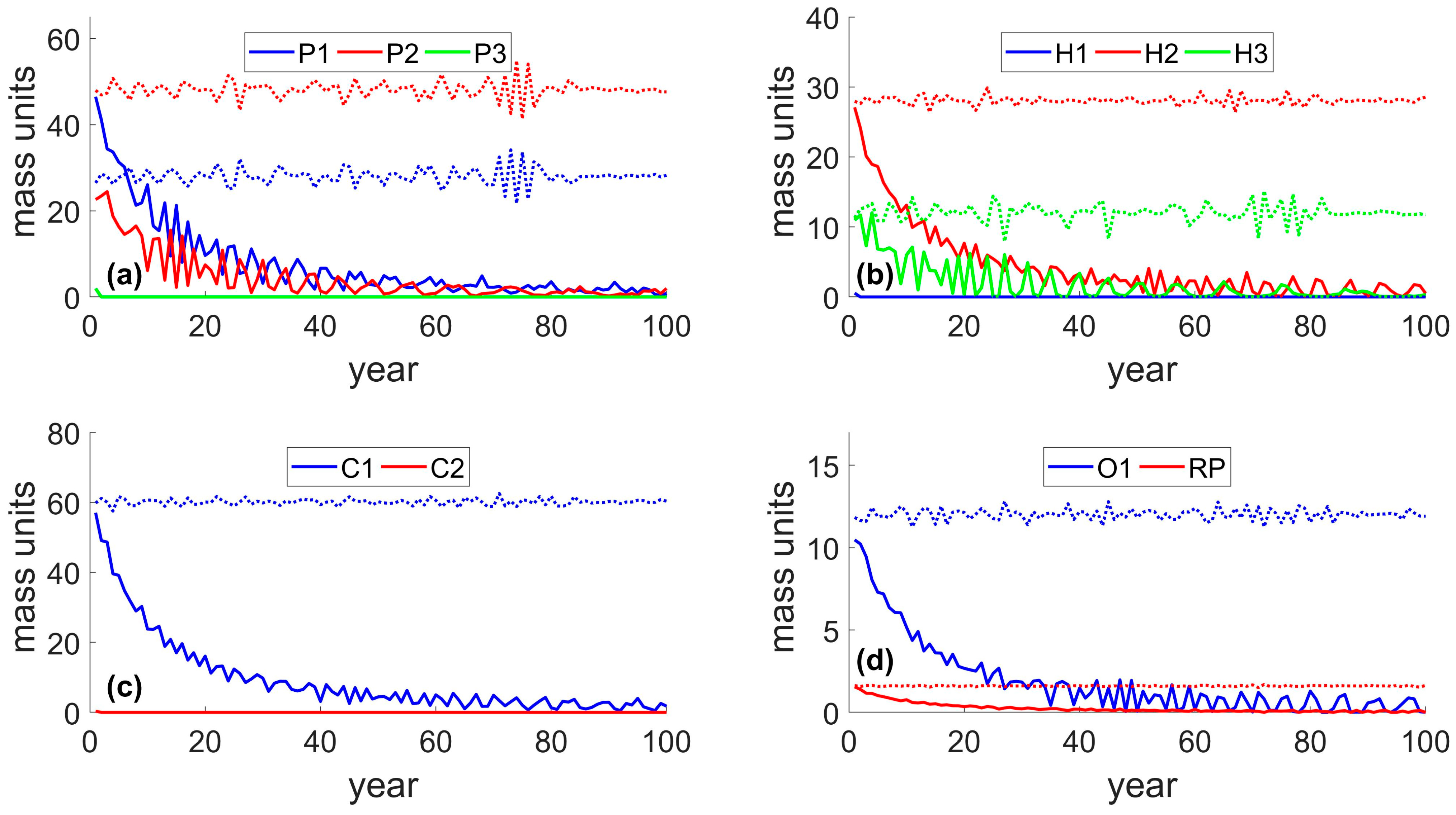
3.3. Case Study 3: Generalized Sustainability Socio–Ecological Model (GSSEM)

The GSSEM monitors GHG atmospheric concentration. Therefore, this variable is used to estimate A_T within the model through Equation (4). All parameters and initial values used for the simulation, along with the corresponding code, can be found in the Supplementary Information. The temperature profile is presented in blue in Figure 16, while the growth factors for the plants are shown in red. Initially, there is a rapid temperature increase, followed by a more gradual but steady rise. This behavior illustrates that when temperatures are near the optimal range, their impact on growth factors is relatively minimal; however, as temperatures continue to rise linearly, the growth factors exhibit an exponential decline. Similarly, Figure 17 contrasts temperature with the human mortality rate. The solid red line represents the baseline death rate profile, which is a time-dependent function reflecting current downward trends. In contrast, the red circle markers indicate the death rate observed in the case study. The figure clearly shows the significant influence of temperature on this parameter, slowing the downward trend until it eventually reverses around year 60.

Unlike in previous case studies, where the temperature remains below 29 °C, this scenario not only reaches but surpasses that threshold within half the simulation period. This rapid escalation is driven by a positive feedback loop, where increasing greenhouse gas (GHG) concentrations and rising temperatures amplify each other, creating a snowball effect that results in a 10 °C temperature rise over the study period. This result, although of higher magnitude, is aligned with the projections made by the IPCC [57]. Furthermore, the last 10 years of the simulation exhibit a dramatic shift in system dynamics, ultimately leading to a system collapse, which will be explored in further detail in the following figures.

Figure 18, Figure 19, Figure 20 and Figure 21 present the compartment performance organized by trophic levels. To facilitate a more accurate and comparative analysis, each compartment was normalized between 0 and 1 based on the case study bounds, given the varying magnitudes of each compartment. In each subplot, solid lines represent the case study results under the influence of global warming, while dashed lines depict the baseline conditions. EP and IS compartments are not shown as they do not accumulate mass; instead, all mass that passes through them is processed and immediately transferred to IRP as waste.

Figure 18 illustrates the plant compartments. P1 represents a domesticated compartment, meaning its dynamics are human-driven through production control. Consequently, its performance closely mirrors the baseline, as its demand is met to the fullest extent possible, even if this requires the overexploitation of resources. In contrast, P2 is the most temperature-sensitive primary producer. The combination of rising system temperatures and overexploitation by H1 results in a sharp decline in P2, culminating in its extinction around year 85. This event triggers an imminent collapse of the entire system within a few years. While a projected nine-decade timeline for a global system collapse may be overstated and unrealistic, the qualitative performance of P1 and P2 aligns with recent findings. Studies by Telo da Gama [67], Cárceles Rodríguez et al. [68] and Davis et al. [69] indicate that current production practices, which focus on sustaining yield levels to meet demand, often at the expense of long-term ecosystem health, reveal that although initial resilience may obscure underlying vulnerabilities, prolonged human intervention can reduce biodiversity and destabilize ecosystems. On the other hand, P3 is far less sensitive to temperature fluctuations. Additionally, under the assumption of a closed-mass system, as in the present approach, and in the absence of human intervention and competition from P2, P3 can grow freely.

Figure 19 presents the herbivore compartments. H1, like P1, is a domesticated species, managed by humans to meet their demand as much as possible. However, despite this control, H1 experiences a dramatic decline, ultimately leading to its extinction when P2, its primary food source, vanishes. H2 relies on both P1 and P2 for sustenance, so its mass declines in parity with the decrease of these compartments. H3 exhibits dynamics like the baseline during the first quarter of the simulation, with a rapid increase. However, it is significantly impacted by the decline of P2, which alters its trajectory and ultimately leads to its imminent extinction by the end of the simulation. In reality, wild herbivores are increasingly endangered due to habitat loss and human activities. Studies such as those by Fetene et al. [70] and Said et al. [71] have determined that livestock expansion directly competes with these animals, restricting their access to essential resources like forage and water. These pressures further fragment habitats, threaten the survival of wild herbivores, and disrupt ecosystems.

Carnivores and humans are analyzed in Figure 20. At the third trophic level, the profiles of carnivores reflect the overall performance of the preceding compartments, resulting in a gradual decline in their mass. This decline culminates in the rapid extinction of C1 during the final phase of the simulation as the system collapses. Carnivores rely on prey populations. When prey species decline, carnivores may struggle to find sufficient food, leading to population reduction [72]. On the other hand, the human population is shown on the right y-axis. In the first half of the simulation period, the case study mirrors the baseline scenario, displaying a growing population that gradually slows down. During the first 30 years, human population growth is around 25%, aligning with United Nations projections that the world population will reach 9.8 billion by 2050, an increase of approximately 23% [73]. However, the shift in the death rate trend becomes evident in the latter half of the simulation, accelerating this slowdown and eventually leading to a decline in the global population. It is important to emphasize that, although this population decline might initially seem beneficial, it is driven by an increase in mortality due to diseases associated with global warming. This aligns with real-world projections from the World Health Organization [74], which indicates that climate change is expected to increase the human death rate in the coming decades due to heat stress, malnutrition, and other climate-related health impacts.

Finally, Figure 21 presents the profiles of the resource pools. The preceding figures indicate an increase in deaths across various compartments, with all this mass being transferred to RP, leading to a significant rise compared to the baseline. In contrast, IRP shows a decrease relative to the reference value as P3 experiences significant growth. This is because P3 serves as the primary mechanism for reintegrating the IRP into the system. Meanwhile, ERP remains largely unchanged, closely mirroring the baseline scenario.

Collectively, the figures illustrate how direct effects propagate through the system, revealing the profound and multifaceted impact of global warming on the ecosystem. This positive feedback mechanism aligns with ecological observations from Visser and Both [43] on the impacts of warming on phenology, where increasing temperatures disrupt life cycle events in primary producers, leading to broader instability across ecosystems. Paiva et al. [62] and Schuur et al. [38] further reinforce these findings, showing that feedback loops in natural systems accelerate the effects of global warming, pushing ecosystems toward rapid degradation. The cascading effects seen in GSSEM mirror these studies, as rising temperatures lead to resource depletion at the primary level, triggering rapid declines in herbivore and carnivore populations. The implications extend to human systems, as highlighted in studies by Ripple et al. [75] and Xu et al. [76], which connect human-driven GHG emissions to ecosystem instability and increased mortality risks. In GSSEM, the human compartment mirrors real-world vulnerabilities, as rising temperatures contribute to increased mortality rates due to climate-related health issues. This underscores that human impacts are both direct and indirect: while emissions drive warming, the resulting ecosystem degradation cycles back to affect human populations.

3.4. Overview of Ecosystem Responses

The results of this study reveal significant insights into the complex interactions between global warming and ecosystem dynamics. The decline of compartment masses across all case studies highlights the critical vulnerabilities of these systems to rising temperatures and resource depletion. Notably, this study underscores how even minor changes at the primary producer level can propagate through the ecosystem, leading to widespread instability and, ultimately, system collapse.

One of the key contributions of this work is the application of a multi-trophic level approach to model the indirect effects of global warming. The observed sharp decline in temperature-sensitive species like P2 mirrors the findings of Paiva et al. [62], who noted similar vulnerabilities in plant species under increasing thermal stress. Additionally, the cascading effects observed in this study are consistent with the trophic cascade theory, where disruptions at lower trophic levels can have far-reaching consequences, as described by Estes et al. [66]. These results reinforce the idea that ecosystems are highly sensitive to changes in temperature and resource availability, which can lead to significant disruptions across multiple trophic levels.

This study highlights the importance of incorporating feedback loops and non-linear dynamics into ecosystem management strategies. The positive feedback loop identified between greenhouse gas emissions and temperature increase is particularly concerning, as it suggests that without intervention, ecosystems may rapidly approach critical thresholds beyond which recovery is unlikely. This underscores the need for proactive measures in climate policy that address the root causes of global warming while also focusing on the resilience of ecosystems [56,75]. The findings support the notion that feedback loops can greatly amplify the effects of global warming, leading to accelerated ecosystem degradation.

While the human population in the model is less directly affected in the short-to-mid-term, the models indicate that it is not immune to the broader ecological disruptions caused by global warming. The eventual decline in the human population, driven by increased mortality rates due to climate-related diseases, is a significant finding. This aligns with research by Xu et al. [76], Song et al. [77], and Pintor [78] which highlights the correlation between rising temperatures and increased mortality rates, particularly among vulnerable populations. This illustrates the indirect but severe consequences of ecosystem degradation on human survival, underscoring the interconnectedness of human and natural systems.

4. Conclusions

The compartmental models presented in this work simulate the cascading impacts of global warming across trophic levels, offering both qualitative and quantitative insights into ecosystem instability under rising temperatures. In the first two case studies, temperature increases of around 3 °C over the simulated period were observed to reduce primary production rates by up to 12%, triggering a sequence of mass declines throughout the system. The third case study showed a more pronounced temperature rise, around 10 °C. Although the anthropic level may exhibit some apparent stability, this results from human efforts to meet their needs by overexploiting natural resources, which accelerates mass losses across trophic levels and leads to an imminent collapse. These results underscore the substantial sensitivity of ecosystem stability to even minor environmental shifts, emphasizing that global warming can drive ecosystems toward irreversible collapse. Quantitative data, such as the rapid 50% biomass loss in certain trophic levels within the first decade or the occurrence of compartment extinction, illustrates the urgent need for proactive climate adaptation strategies.

Given these findings, this study highlights the essential role of feedback loops and non-linear interactions in ecological systems. The integration of greenhouse gas (GHG) emissions, temperature anomaly, and vegetative growth within the model underscores how interconnected factors like rising temperatures and habitat loss amplify each other, increasing ecosystem vulnerability. This supports the need for adaptive management strategies that consider ecological thresholds and tipping points. For instance, implementing adaptive practices that target the resilience of temperature-sensitive compartments, like primary producers, could help mitigate the risk of cascade effects on higher trophic levels. By quantitatively demonstrating the rapid destabilization possible in these systems, this study advocates for sustainable management practices that can buffer these effects before ecosystems reach critical limits.

Despite the usefulness demonstrated by the compartmental approach, several limitations of this study should be acknowledged. The models rely on simplifying assumptions, such as the homogeneity of compartments and the exclusion of stochastic events, which may limit their ability to fully capture the complexity of real-world ecosystems. Additionally, GSSEM uses a combination of conceptual and real-world parameters, which reduces the precision of its numerical predictions. As a result, the findings are primarily qualitative, offering significant insights into the internal mechanisms of human ecosystems but not providing exact timelines or magnitudes of change. Therefore, while the model effectively illustrates the relationships and influences between system components, its generalizability is constrained and may not fully reflect precise real-world outcomes. Nevertheless, despite these limitations, this study offers a valuable and comprehensive qualitative analysis of the indirect effects of global warming on ecosystems. It highlights the critical need to develop and continuously refine models to improve the analysis, monitoring, control, and prediction of ecosystem dynamics.

Moving forward, it is essential to integrate ecological, social, and economic considerations into policy-making to ensure the long-term sustainability of both natural and human systems. The IPCC highlights the critical role of adaptive strategies in managing climate-induced ecosystem risks. To achieve this, decision-makers should adopt specific and comprehensive strategies. The findings of this study make it clear that temperature-sensitive primary producers, which serve as foundational elements of ecosystems, require particular protection. Adaptive land management practices, such as reforestation, habitat restoration, and soil conservation, are essential for enhancing resilience. The findings also indicate that the feedback loop is triggered by GHG emissions. The UNEP recommends integrating biodiversity conservation with climate mitigation to enhance ecosystem adaptability under warming conditions. In this context, implementing carbon pricing, incentivizing green finance, adopting circular economy models, and investing in renewable energy solutions can address the root causes of GHG emissions, thereby reducing the likelihood of severe warming feedback loops. Moreover, enhancing public health infrastructure to address climate-related risks, such as heat waves and vector-borne diseases, will be critical to protecting vulnerable populations. By combining such practical strategies, resource management will become more effective, mitigating the impacts of global warming and safeguarding the delicate balance of ecosystems.

References

1. Rockström, J.; Steffen, W.; Noone, K.; Persson, Å.; Chapin, F.S., III; Lambin, E.F.; Lenton, T.M.; Scheffer, M.; Folke, C.; Schellnhuber, H.J.; et al. A safe operating space for humanity. Nature 2009, 461, 472–475. [Google Scholar] [CrossRef]
2. Steffen, W.; Richardson, K.; Rockström, J.; Cornell, S.E.; Fetzer, I.; Bennett, E.M.; Biggs, R.; Carpenter, S.R.; De Vries, W.; De Wit, C.A.; et al. Planetary boundaries: Guiding human development on a changing planet. Science 2015, 347, 1259855. [Google Scholar] [CrossRef]
3. Varotsos, C.; Efstathiou, M. Has global warming already arrived? J. Atmos. Solar-Terr. Phys. 2019, 182, 31–38. [Google Scholar] [CrossRef]
4. Hughes, L. Biological consequences of global warming: Is the signal already apparent? Trends Ecol. Evol. 2000, 15, 56–61. [Google Scholar] [CrossRef]
5. Coudrain, A.; Francou, B.; Kundzewicz, Z.W. Glacier shrinkage in the Andes and consequences for water resources—Editorial. Hydrol. Sci. J. 2005, 50, 925–932. [Google Scholar] [CrossRef]
6. Elewa, A.M.; Abdelhady, A.A. Past, present, and future mass extinctions. J. Afr. Earth Sci. 2020, 162, 103678. [Google Scholar] [CrossRef]
7. Prăvălie, R. Major perturbations in the Earth’s forest ecosystems. Possible implications for global warming. Earth-Sci. Rev. 2018, 185, 544–571. [Google Scholar] [CrossRef]
8. Lippmann, R.; Babben, S.; Menger, A.; Delker, C.; Quint, M. Development of Wild and Cultivated Plants under Global Warming Conditions. Curr. Biol. 2019, 29, R1326–R1338. [Google Scholar] [CrossRef]
9. Sun, Q.; Miao, C.; Hanel, M.; Borthwick, A.G.; Duan, Q.; Ji, D.; Li, H. Global heat stress on health, wildfires, and agricultural crops under different levels of climate warming. Environ. Int. 2019, 128, 125–136. [Google Scholar] [CrossRef]
10. Fattorini, S. Climate Change and Extinction Events. In Encyclopedia of Geology, Volume 1–6, 2nd ed.; Elsevier: Amsterdam, The Netherlands, 2021; Volume 5, pp. 585–595. [Google Scholar] [CrossRef]
11. Rodriguez-Gonzalez, P.T.; Rico-Martinez, R.; Rico-Ramirez, V. Effect of feedback loops on the sustainability and resilience of human-ecosystems. Ecol. Model. 2020, 426, 109018. [Google Scholar] [CrossRef]
12. Zhou, T.; Huang, X.; Zhang, N. Does the high-speed railway make cities more carbon efficient? Evidence from the perspective of the spatial spillover effect. Environ. Impact Assess. Rev. 2023, 101, 107137. [Google Scholar] [CrossRef]
13. Gao, D.; Mo, X.; Xiong, R.; Huang, Z. Tax Policy and Total Factor Carbon Emission Efficiency: Evidence from China’s VAT Reform. Int. J. Environ. Res. Public Health 2022, 19, 9257. [Google Scholar] [CrossRef]
14. Sinha, E. Identifying enablers and outcomes of circular economy for sustainable development: A systematic literature review. Bus. Strat. Dev. 2022, 5, 232–244. [Google Scholar] [CrossRef]
15. Mamun, A.; Boubaker, S.; Nguyen, D.K. Green finance and decarbonization: Evidence from around the world. Financ. Res. Lett. 2022, 46, 102807. [Google Scholar] [CrossRef]
16. Martinho, V.J.P.D. European Union farming systems: Insights for a more sustainable land use. Land Degrad. Dev. 2022, 33, 527–544. [Google Scholar] [CrossRef]
17. Foley, J.A.; DeFries, R.; Asner, G.P.; Barford, C.; Bonan, G.; Carpenter, S.R.; Chapin, F.S.; Coe, M.T.; Daily, G.C.; Gibbs, H.K.; et al. Global consequences of land use. Science 2005, 309, 570–574. [Google Scholar] [CrossRef]
18. Ostrom, E. A General framework for analyzing sustainability of social-ecological systems. Science 2009, 325, 419–422. [Google Scholar] [CrossRef]
19. Boccara, N. Modeling Complex Systems; Springer Nature: Dordrecht, The Netherlands, 2010; ISBN 9781441965615. [Google Scholar]
20. Yang, Y. Sustainability Analysis of Enterprise Performance Management Driven by Big Data and Internet of Things. Sustainability 2023, 15, 4839. [Google Scholar] [CrossRef]
21. Nisal, A.; Diwekar, U.; Hanumante, N.; Shastri, Y.; Cabezas, H. Integrated model for food-energy-water (FEW) nexus to study global sustainability: The main generalized global sustainability model (GGSM). PLoS ONE 2022, 17, e0267403. [Google Scholar] [CrossRef] [PubMed]
22. Monteiro, N.; Pinheiro, S.; Magalhães, S.; Tarroso, P.; Vincent, A. Predicting the impacts of climate change on the distribution of European syngnathids over the next century. Front. Mar. Sci. 2023, 10, 1138657. [Google Scholar] [CrossRef]
23. Diwekar, U.; Nisal, A.; Shastri, Y.; Cabezas, H. Optimal Control for Deriving Policies for Global Sustainability. Comput. Aided Chem. Eng. 2023, 52, 2471–2476. [Google Scholar] [CrossRef]
24. Flensborg, L.C.; A Maureaud, A.; Bravo, D.N.; Lindegren, M. An indicator-based approach for assessing marine ecosystem resilience. ICES J. Mar. Sci. 2023, 80, 1487–1499. [Google Scholar] [CrossRef]
25. Pindyck, R.S. The Use and Misuse of Models for Climate Policy. Rev. Environ. Econ. Policy 2017, 11, 100–114. [Google Scholar] [CrossRef]
26. Weyant, J. Some Contributions of Integrated Assessment Models of Global Climate Change. Rev. Environ. Econ. Policy 2017, 11, 115–137. [Google Scholar] [CrossRef]
27. Stehfest, E.; van Vuuren, D.; Kram, T.; Bouwman, L. Integrated Assessment of Global Environmental Change with IMAGE 3.0: Model Description and Policy Applications. The Hague: PBL Netherlands Environmental Assessment Agency; 2014. Available online: https://www.pbl.nl/sites/default/files/downloads/pbl-2014-integrated_assessment_of_global_environmental_change_with_image30_735.pdf (accessed on 27 August 2024).
28. Calvin, K.; Patel, P.; Clarke, L.; Asrar, G.; Bond-Lamberty, B.; Cui, R.Y.; Di Vittorio, A.; Dorheim, K.; Edmonds, J.; Hartin, C.; et al. GCAM v5.1: Representing the linkages between energy, water, land, climate, and economic systems. Geosci. Model. Dev. 2019, 12, 677–698. [Google Scholar] [CrossRef]
29. King, C.W. An integrated biophysical and economic modeling framework for long-term sustainability analysis: The HARMONEY model. Ecol. Econ. 2019, 169, 106464. [Google Scholar] [CrossRef]
30. Jørgensen, S.E.; Fath, B.D. Fundamentals of Ecological Modelling: Applications in Environmental Management and Research, 4th ed.; Elsevier: Amsterdam, The Netherlands, 2011. [Google Scholar]
31. Bertozzi, A.L.; Franco, E.; Mohler, G.; Short, M.B.; Sledge, D. The challenges of modeling and forecasting the spread of COVID-19. Proc. Natl. Acad. Sci. USA 2020, 117, 16732–16738. [Google Scholar] [CrossRef]
32. Mwalili, S.; Kimathi, M.; Ojiambo, V.; Gathungu, D.; Mbogo, R. SEIR model for COVID-19 dynamics incorporating the environment and social distancing. BMC Res. Notes 2020, 13, 1–5. [Google Scholar] [CrossRef]
33. He, S.; Peng, Y.; Sun, K. SEIR modeling of the COVID-19 and its dynamics. Nonlinear Dyn. 2020, 101, 1667–1680. [Google Scholar] [CrossRef]
34. Rodriguez-Gonzalez, P.T.; Rico-Martinez, R.; Rico-Ramirez, V. An integrated stochastic economic-ecological-social model with stratified-population. Ecol. Model. 2018, 368, 15–26. [Google Scholar] [CrossRef]
35. Nisal, A.; Diwekar, U.; Hanumante, N.; Shastri, Y.; Cabezas, H.; Ramirez, V.R.; Rodríguez-González, P.T. Evaluation of global techno-socio-economic policies for the FEW nexus with an optimal control based approach. Front. Sustain. 2022, 3, 948443. [Google Scholar] [CrossRef]
36. Hanumante, N.; Shastri, Y.; Nisal, A.; Diwekar, U.; Cabezas, H. Water stress-based price for global sustainability: A study using generalized global sustainability model (GGSM). Clean Technol. Environ. Policy 2024, 1–20. [Google Scholar] [CrossRef]
37. Jones, M.C.; Grosse, G.; Treat, C.; Turetsky, M.; Anthony, K.W.; Brosius, L. Past permafrost dynamics can inform future permafrost carbon-climate feedbacks. Commun. Earth Environ. 2023, 4, 272. [Google Scholar] [CrossRef]
38. Schuur, E.A.; Abbott, B.W.; Commane, R.; Ernakovich, J.; Euskirchen, E.; Hugelius, G.; Grosse, G.; Jones, M.; Koven, C.; Leshyk, V.; et al. Permafrost and Climate Change: Carbon Cycle Feedbacks From the Warming Arctic. Annu. Rev. Environ. Resour. 2022, 47, 343–371. [Google Scholar] [CrossRef]
39. Kimmins, H.; Blanco, J.A.; Seely, B.; Welham, C.; Scoullar, K. Forecasting Forest Futures: A Hybrid Modelling Approach to the Assessment of Sustainability of Forest Ecosystems and Their Values; Routledge: Oxfordshire, UK, 2010; pp. 1–281. [Google Scholar] [CrossRef]
40. Martin, R.; Schlüter, M. Combining system dynamics and agent-based modeling to analyze social-ecological interactions—An example from modeling restoration of a shallow lake. Front. Environ. Sci. 2015, 3, 66. [Google Scholar] [CrossRef]
41. Dong, L.; Huang, Z. Some evidence and new insights for feedback loops of human-nature interactions from a holistic Earth perspective. J. Clean. Prod. 2023, 432, 139667. [Google Scholar] [CrossRef]
42. Ripple, W.J.; Wolf, C.; Lenton, T.M.; Gregg, J.W.; Natali, S.M.; Duffy, P.B.; Rockström, J.; Schellnhuber, H.J. Many risky feedback loops amplify the need for climate action. One Earth 2023, 6, 86–91. [Google Scholar] [CrossRef]
43. E Visser, M.; Both, C. Shifts in phenology due to global climate change: The need for a yardstick. Proc. R. Soc. B Biol. Sci. 2005, 272, 2561–2569. [Google Scholar] [CrossRef]
44. Janni, M.; Maestri, E.; Gullì, M.; Marmiroli, M.; Marmiroli, N. Plant responses to climate change, how global warming may impact on food security: A critical review. Front. Plant Sci. 2023, 14, 1297569. [Google Scholar] [CrossRef]
45. I Zandalinas, S.; Balfagón, D.; Gómez-Cadenas, A.; Mittler, R. Plant responses to climate change: Metabolic changes under combined abiotic stresses. J. Exp. Bot. 2022, 73, 3339–3354. [Google Scholar] [CrossRef]
46. Schmitz, O.J.; Hambäck, P.A.; Beckerman, A.P. Trophic Cascades in Terrestrial Systems: A Review of the Effects of Carnivore Removals on Plants. Am. Nat. 2000, 155, 141–153. [Google Scholar] [CrossRef] [PubMed]
47. Gonzalez, P.; Tucker, C.; Sy, H. Tree density and species decline in the African Sahel attributable to climate. J. Arid. Environ. 2012, 78, 55–64. [Google Scholar] [CrossRef]
48. Hasibuan, A.; Supriatna, A.K.; Rusyaman, E.; Biswas, H.A. Harvested Predator–Prey Models Considering Marine Reserve Areas: Systematic Literature Review. Sustainability 2023, 15, 12291. [Google Scholar] [CrossRef]
49. Korobeinikov, A. Stability of ecosystem: Global properties of a general predator-prey model. Math. Med. Biol. A J. IMA 2009, 26, 309–321. [Google Scholar] [CrossRef]
50. Kotecha, P.; Diwekar, U.; Cabezas, H. Model-based approach to study the impact of biofuels on the sustainability of an ecological system. Clean Technol. Environ. Policy 2013, 15, 21–33. [Google Scholar] [CrossRef]
51. Shastri, Y.; Diwekar, U.; Cabezas, H.; Williamson, J. Is sustainability achievable? Exploring the limits of sustainability with model systems. Environ. Sci. Technol. 2008, 42, 6710–6716. [Google Scholar] [CrossRef]
52. Chapra, S.C.; Canale, R.P. Numerical Methods for Engineers, 6th ed.; McGraw-Hill: New York, NY, USA, 2010. [Google Scholar]
53. Pawlowski, C.W.; Fath, B.D.; Mayer, A.L.; Cabezas, H. Towards a sustainability index using information theory. Energy 2005, 30, 1221–1231. [Google Scholar] [CrossRef]
54. Lotka, A.J. Elements of Physical Biology; Williams and Wilkins: Philadelphia, PA, USA, 1925. [Google Scholar]
55. Volterra, V. Variazioni e fluttuazioni del numero d’individui in specie animali conviventi. Mem. Della R. Accad. Naz. Dei Lincei 1926, 2, 31–113. [Google Scholar]
56. Intergovernmental Panel on Climate Change (IPCC). Impacts of 1.5 °C Global Warming on Natural and Human Systems. In Global Warming of 1.5 °C: IPCC Special Report on Impacts of Global Warming of 1.5 °C Above Pre-Industrial Levels in Context of Strengthening Response to Climate Change, Sustainable Development, and Efforts to Eradicate Poverty; Cambridge University Press: Cambridge, UK, 2022; pp. 175–312. [Google Scholar]
57. I. P. on C. C. (IPCC). Climate Change 2021—The Physical Science Basis: Working Group I Contribution to the Sixth Assessment Report of the Intergovernmental Panel on Climate Change. In Climate Change 2021—The Physical Science Basis; Cambridge University Press: Cambridge, UK, 2023. [Google Scholar] [CrossRef]
58. I. P. on C. C. (IPCC). Climate Change 2022—Impacts, Adaptation and Vulnerability: Working Group II Contribution to the Sixth Assessment Report of the Intergovernmental Panel on Climate Change. In Climate Change 2022—Impacts, Adaptation and Vulnerability; Cambridge University Press: Cambridge, UK, 2023. [Google Scholar] [CrossRef]
59. NOAA Global Monitoring Laboratory—THE NOAA ANNUAL GREENHOUSE GAS INDEX (AGGI). Available online: https://gml.noaa.gov/aggi/aggi.html (accessed on 27 August 2024).
60. Data.GISS: GISS Surface Temperature Analysis (GISTEMP v4). Available online: https://data.giss.nasa.gov/gistemp/ (accessed on 27 August 2024).
61. Nahar, K.; Hasanuzzaman, M.; Ahamed, K.U.; Hakeem, K.R.; Ozturk, M.; Fujita, M. Plant Responses and Tolerance to High Temperature Stress: Role of Exogenous Phytoprotectants. In Crop Production and Global Environmental Issues; Springer: Berlin/Heidelberg, Germany, 2015; pp. 385–435. [Google Scholar] [CrossRef]
62. Paiva, S.L.; Savi, M.A.; Viola, F.M.; Leiroz, A.J. Global warming description using Daisyworld model with greenhouse gases. Biosystems 2014, 125, 1–15. [Google Scholar] [CrossRef]
63. Lin, Y.-S.; Medlyn, B.E.; Ellsworth, D.S. Temperature responses of leaf net photosynthesis: The role of component processes. Tree Physiol. 2012, 32, 219–231. [Google Scholar] [CrossRef]
64. O’Sullivan, O.S.; Heskel, M.A.; Reich, P.B.; Tjoelker, M.G.; Weerasinghe, L.K.; Penillard, A.; Zhu, L.; Egerton, J.J.G.; Bloomfield, K.J.; Creek, D.; et al. Thermal limits of leaf metabolism across biomes. Glob. Chang. Biol. 2017, 23, 209–223. [Google Scholar] [CrossRef] [PubMed]
65. Rocklöv, J.; Ebi, K.; Forsberg, B. Mortality Related to Temperature and Persistent Extreme Temperatures—A Study of Cause-Specific and Age Stratified Mortality. Epidemiology 2011, 22, S13. [Google Scholar] [CrossRef]
66. Estes, J.A.; Terborgh, J.; Brashares, J.S.; Power, M.E.; Berger, J.; Bond, W.J.; Carpenter, S.R.; Essington, T.E.; Holt, R.D.; Jackson, J.B.C.; et al. Trophic downgrading of planet earth. Science 2011, 333, 301–306. [Google Scholar] [CrossRef]
67. da Gama, J.T. The Role of Soils in Sustainability, Climate Change, and Ecosystem Services: Challenges and Opportunities. Ecologies 2023, 4, 552–567. [Google Scholar] [CrossRef]
68. Rodríguez, B.C.; Durán-Zuazo, V.H.; Rodríguez, M.S.; García-Tejero, I.F.; Ruiz, B.G.; Tavira, S.C. Conservation Agriculture as a Sustainable System for Soil Health: A Review. Soil Syst. 2022, 6, 87. [Google Scholar] [CrossRef]
69. Davis, A.S.; Hill, J.D.; Chase, C.A.; Johanns, A.M.; Liebman, M. Increasing Cropping System Diversity Balances Productivity, Profitability and Environmental Health. PLoS ONE 2012, 7, e47149. [Google Scholar] [CrossRef] [PubMed]
70. Fetene, A.; Yeshitela, K.; Gebremariam, E. The effects of anthropogenic landscape change on the abundance and habitat use of terrestrial large mammals of Nech Sar National Park. Environ. Syst. Res. 2019, 8, 19. [Google Scholar] [CrossRef]
71. Said, M.Y.; Ogutu, J.O.; Kifugo, S.C.; Makui, O.; Reid, R.S.; de Leeuw, J. Effects of extreme land fragmentation on wildlife and livestock population abundance and distribution. J. Nat. Conserv. 2016, 34, 151–164. [Google Scholar] [CrossRef]
72. Stirling, I.; Derocher, A.E. Effects of climate warming on polar bears: A review of the evidence. Glob. Chang. Biol. 2012, 18, 2694–2706. [Google Scholar] [CrossRef]
73. World Population Prospects—Population Division—United Nations. Available online: https://population.un.org/wpp/ (accessed on 27 August 2024).
74. Climate Change. Available online: https://www.who.int/news-room/fact-sheets/detail/climate-change-and-health (accessed on 24 October 2024).
75. Ripple, W.J.; Wolf, C.; Newsome, T.M.; Barnard, P.; Moomaw, W.R. World Scientists’ Warning of a Climate Emergency. Bioscience 2020, 70, 8–12. [Google Scholar] [CrossRef]
76. Xu, Z.; Sheffield, P.E.; Hu, W.; Su, H.; Yu, W.; Qi, X.; Tong, S. Climate Change and Children’s Health—A Call for Research on What Works to Protect Children. Int. J. Environ. Res. Public Health 2012, 9, 3298–3316. [Google Scholar] [CrossRef] [PubMed]
77. Song, X.; Wang, S.; Hu, Y.; Yue, M.; Zhang, T.; Liu, Y.; Tian, J.; Shang, K. Impact of ambient temperature on morbidity and mortality: An overview of reviews. Sci. Total. Environ. 2017, 586, 241–254. [Google Scholar] [CrossRef] [PubMed]
78. Pintor, M.P. The future of the temperature–mortality relationship. Lancet Public Health 2024, 9, e636–e637. [Google Scholar] [CrossRef] [PubMed]
Figure 1. Generalized scheme of the Lotka–Volterra compartmental model.
World 05 00054 g001
Figure 2. Basic scheme of a multi-predator–prey model.
World 05 00054 g002
Figure 3. Scheme of the multi-level predator–prey model.
World 05 00054 g003
Figure 4. Graphic representation of the human ecosystem model.
World 05 00054 g004
Figure 5. Conceptualized chain of effects driven by greenhouse gas (GHG) emissions.
World 05 00054 g005
Figure 6. Schematization of the global warming feedback loop.
World 05 00054 g006
Figure 7. Temperature anomaly fitting as time-function.
World 05 00054 g007
Figure 8. Temperature anomaly—CO2eq fitting.
World 05 00054 g008
Figure 9. Plant growth rate and human mortality rate as function of temperature.
World 05 00054 g009
Figure 10. Cycle period of all species in case study 1.
World 05 00054 g010
Figure 11. Temperature and growth factor of case study 1.
World 05 00054 g011
Figure 12. Compartment profiles of case study 1.
World 05 00054 g012
Figure 13. Cycle period of P1 in case study 2.
World 05 00054 g013
Figure 14. Temperature and growth factors for case study 2.
World 05 00054 g014
Figure 15. Compartment profiles of case study 2: (a) plant compartments, (b) herbivore compartments, (c) carnivore compartments, and (d) omnivore and resource pool compartments.
World 05 00054 g015
Figure 16. Temperature and plant growth factors for case study 3.
World 05 00054 g016
Figure 17. Temperature and human death rate for case study 3.
World 05 00054 g017
Figure 18. Plant compartment profiles for case study 3.
World 05 00054 g018
Figure 19. Herbivore compartment profiles for case study 3.
World 05 00054 g019
Figure 20. Carnivores and human profiles for case study 3.
World 05 00054 g020
Figure 21. Resource pool profiles for case study 3.
World 05 00054 g021