Effect of Different Irrigation Managements on Infiltration Equations and Their Coefficients

Abstract

The main aim of this paper was to analyze the sensitivity of the five infiltration equations (Kostiakov, Kostiakov–Lewis, Philip, Horton and SCS) and their coefficients to various ponding depths and initial soil moisture under different irrigation managements. The treatments included three qualities of water (electrical conductivity = 6, 3 and 0.6 dS/m), two managements of irrigation (intermittent irrigation and daily irrigation) and three irrigation periods (100, 45 and 8 days). The HYDRUS-1D model was calibrated to simulate infiltration in various initial soil moistures and ponding depths. Evaluating the performance of infiltration equations showed that the Horton and Kostiakov–Lewis had better accuracy and Kostiakov and SCS had less accuracy than the other equations. The empirical coefficients of SCS and Kostiakov had the most and least sensitivities, respectively. Furthermore, Horton was the most sensitive equation, while SCS was the least sensitive one. The output parameters under daily management were the most sensitive to variations in infiltration coefficients, especially when the salinity and sodium contents of water and soil were higher. The results also showed that the effect of the initial soil moisture on the infiltration coefficient in high permeable soil (arising from daily management) was greater; but in low permeable soil (arising from intermittent management), the ponding depth was more effective. It is concluded that the infiltration equations (specifically the SCS equation) and their coefficients (specifically coefficient c) should be calibrated relative to the initial soil moisture, ponding depth, soil solution and water irrigation quality. Particularly in areas with high permeable soil (in the daily management), the calibration of the infiltration equation should be conducted with the initial soil moisture. In these areas, the irrigation period should be controlled. In areas with low permeable soil (in intermittent management), calibration should be carried out relative to the ponding depth. In these areas, the inflow rate should be controlled.

1. Introduction

Infiltration equations are important to evaluate soil hydrologic characteristics and surface irrigation performance [1,2]. To date, various infiltration equations have been presented. Nevertheless, few of these equations can provide a clear analysis [3]. The calculation of the infiltration coefficient is the principal criterion to prefer one equation over others [4]. The permeability process can be accurately determined with the appropriate set of permeability coefficients [5], and these coefficients are affected by irrigation management, soil moisture, water head and the quality of the irrigation water [6,7,8]. Considering the problems of infiltration measurement (expensive and time-consuming) and the variability of infiltration coefficients, it is necessary to determine the equation that has the least error while being the most sensitive equation to changes in conditions. Via the most sensitive equation, they can estimate the infiltration value with good accuracy [9]. Malik et al. (1992) investigated the soil sodium and calcium effects against soil dispersion and swelling. They observed that as the sodium adsorption ratio (SAR) increased, the unsaturated hydraulic conductivity decreased [10]. The effects of irrigation water quality on infiltration in a sandy loam soil using the rainfall simulator revealed that the maximum infiltration occurred at an electrical conductivity (EC) of 5 dS/m and SAR of 5 [11]. Sepaskhah and Afshar-Chamanabad (2002) indicated that the coefficients of the Kostiakov–Lewis equation in furrow irrigation should be adjusted based on the furrow inflow rate (i.e., water depth) [12]. Shukla et al. (2003) showed that the use of land, tillage practices and manure usage led to remarkable effects on infiltration equations [13]. Dagadu and Nimbalkar (2012) evaluated Green-Ampt, modified Kostiakov, Horton and Kostiakov infiltration equations. The results showed that Horton’s equation and the Green-Ampt equation were best fitted to the observed field data to estimate infiltration rates at any given time with a high degree of correlation coefficient and the minimum degree of standard error [14]. The effects of EC and SAR on infiltration rates found that it reduced greatly by raising EC and SAR soil [6]. Babaei et al. (2018) indicated that the infiltration had a large spatial variation in the arid regions [4]. Turner (2006) indicated that the final intake rate coefficient of the Horton equation and the soil sorptivity coefficient of the Philip equation was more sensitive compared to other coefficients [15]. Javadi et al. (2014) indicated the sensitivity of the coefficients of the Horton, Kostiakov–Lewis and Philip equations to different initial soil moistures and water heads in surface irrigation for one and two-dimensional infiltration conditions by the HYDRUS (v 4.11). They showed that the soil sorptivity coefficient of the Philip equation was more sensitive to the initial soil moisture and ponding depth. The Horton equation was the most sensitive equation and the Kostiakov–Lewis and Philip equations for two-dimensional and one-dimensional conditions had similar sensitivities [16]. Hoyos and Cavalcante (2015) found that the coefficient of the Kostiakov and the Horton equations were the most sensitive coefficient and equation, respectively [17]. Sepah Vand et al., 2018 analyzed the sensitivity of the infiltration rate to the removal of one input parameter (time, percentage of silt, clay, sand, moisture content and bulk density and in per centimeter). It can be concluded that the time parameter has the greatest effect on the estimation of the infiltration rate [18]. Infiltration coefficients can be measured in the lab and farm, which is difficult and expensive [19,20]. Therefore, indirect ways have been suggested to estimate coefficients; modeling is one of these ways [21]. In recent decades, one of the models that has been widely used in estimating soil hydraulic parameters is the HYDRUS model. The findings of Mashayekhi et al. (2016) showed that by reducing the parameters involved in the optimization of soil hydraulic parameters, the simulation accuracy can be increased [22]. Furthermore, Zheng et al. (2017) reported that HYDRUS was a powerful tool to inversely estimate hydraulic properties if we give proper and accurate information in the objective function [23]. The review of the research showed that the behavior of infiltration equations is different in various irrigation management and agricultural conditions, and under specific evaluation conditions, each equation is superior to other equations. This is important because the infiltration function is assumed to be fixed during the season, whereas the irrigation duration (initial soil moisture) and inflow rate to the field (ponding depth) change throughout the season. Accordingly, the infiltration coefficients are variable during the season, and assuming constant infiltration coefficients reduces the performance of surface irrigation.

The results of the literature review showed that the parameters affecting soil permeability, such as initial soil moisture and ponding depth, change during the irrigation season, so the use of constant infiltration coefficients reduces irrigation efficiency [6]. Therefore, the irrigation efficiency of systems can be improved by identification and calibration of the most sensitive coefficients to the variation in initial soil moisture and ponding depth. Unfortunately, few studies have been conducted on the simultaneous effect of irrigation water quality, irrigation period and soil moisture management on infiltration coefficients. Therefore, the main goal of this paper was to study the most sensitive infiltration coefficients under different irrigation managements related to various initial soil moisture and ponding depth. The aim of this study is as follows:

• To use soil columns to measure cumulative infiltration under various irrigation treatments;
• To calculate the soil hydraulic parameters and infiltration in various initial soil moistures and water heads with the HYDRUS-1D model;
• To determine the coefficients of the infiltration equations and identify the most sensitive infiltration equations and their coefficients relative to different initial soil moistures and water heads.

2. Materials and Methods

2.1. Methodology

This research included two parts, including infiltration experiments and modeling. First, the water infiltration was measured under a fixed ponding depth via soil columns; then, the HYDRUS-1D model was calibrated for the situations of the experimental study. Next, the HYDRUS-1D model was adjusted for simulating infiltration to different initial soil moistures and ponding depths under different irrigation managements.

2.2. Experimental Design

In this research, an experimental design with a factorial completely randomized design was used. According to

Table 1. Experimental treatments used in this study.

Description	Treatment
Low saline–sodic (Qg; SAR = 0.77 (meq L−1)−0.5 and EC = 0.6 dS m−1)	Irrigation water quality (Q)
Medium saline–sodic (Qm; SAR = 11.30 (meq L−1)−0.5 and EC = 3.0 dS m−1)
High saline–sodic (Qh; SAR = 21.38 (meq L−1)−0.5 and EC = 6.0 dS m−1)
Intermittent (Mi)	Management of irrigation (M)
Daily (Md)
The end of period (100 days, Ib)	Period of the irrigation (I)
The middle of period (45 days, Im)
The beginning of period (8 days, Ib)

, the treatments were based on three qualities of water, two managements of irrigation and three periods of irrigation with four replications. The fourth replication was applied as a control treatment and sampling before the infiltration experiment. The end (I_e), middle (I_m) and beginning of the irrigation period (I_b) were 100, 45 and 8 days, respectively. The sandy loam soil was used. The chemical and physical characteristics of the soil are presented in

Table 2. Average amounts of chemical and physical characteristics of the soil.

Value	Soil Properties
55	Sand (kg 100 kg−1)
15	Clay (kg 100 kg−1)
30	Silt (kg 100 kg−1)
1.60	Bulk density (g/cm3)
0.094	Hydraulic conductivity (cm/min)
0.65	Sodium adsorption ratio; SARe ((meq·L−1)−0.5)
0.72	Electrical conductivity of the saturated extract; ECe (dS/m)
7.37	pH

. Due to the amounts of soil hydraulic conductivity, sodium adsorption ratio (SAR_e) and the saturated extract’s electrical conductivity (EC_e), the soil has medium permeability and has a non-saline sodic quality. The saline water was created by increasing the needed amounts of calcium chloride and sodium chloride to the distilled water.

2.3. Irrigation Management

In this study, two irrigation managements were applied (

Table 3. Descriptions of two irrigation managements.

Irrigation Management	Irrigation Period	θFC (m3m−3)	Irrigation (mm/Event)	Mean of Irrigation Interval (Day)	Amount of Irrigation Events	Period of Irrigation (Days)	Leaching Fraction with Irrigation (%)	Infiltration Experiment Time (Days)
Mi	Ib	0.153	18.1	8	1	8	-	16
	Im	0.146	17.3	9	5	45	-	56
	Ie	0.151	17.9	10	10	100	-	114
Md	Ib	0.153	2 to 3.1	1	8	8	15	16
	Im	0.146	2 to 3.1	1	45	45	15	56
	Ie	0.151	2 to 3.1	1	100	100	15	114

):

• Intermittent (M_i): Irrigation is performed when the soil moisture reaches 70% of field capacity (FC) (management of conventional). By the weighing procedure, the soil moisture was calculated.
• Daily (M_d): To avoid an excessive buildup of solutes in the soil columns, the soil was irrigated daily with a fraction of leaching (LF) of 0.15 (management of ideal).

After every irrigation under both managements, the soil moisture reached FC, and the soil moisture reduction was due to the evaporation of the soil surface.

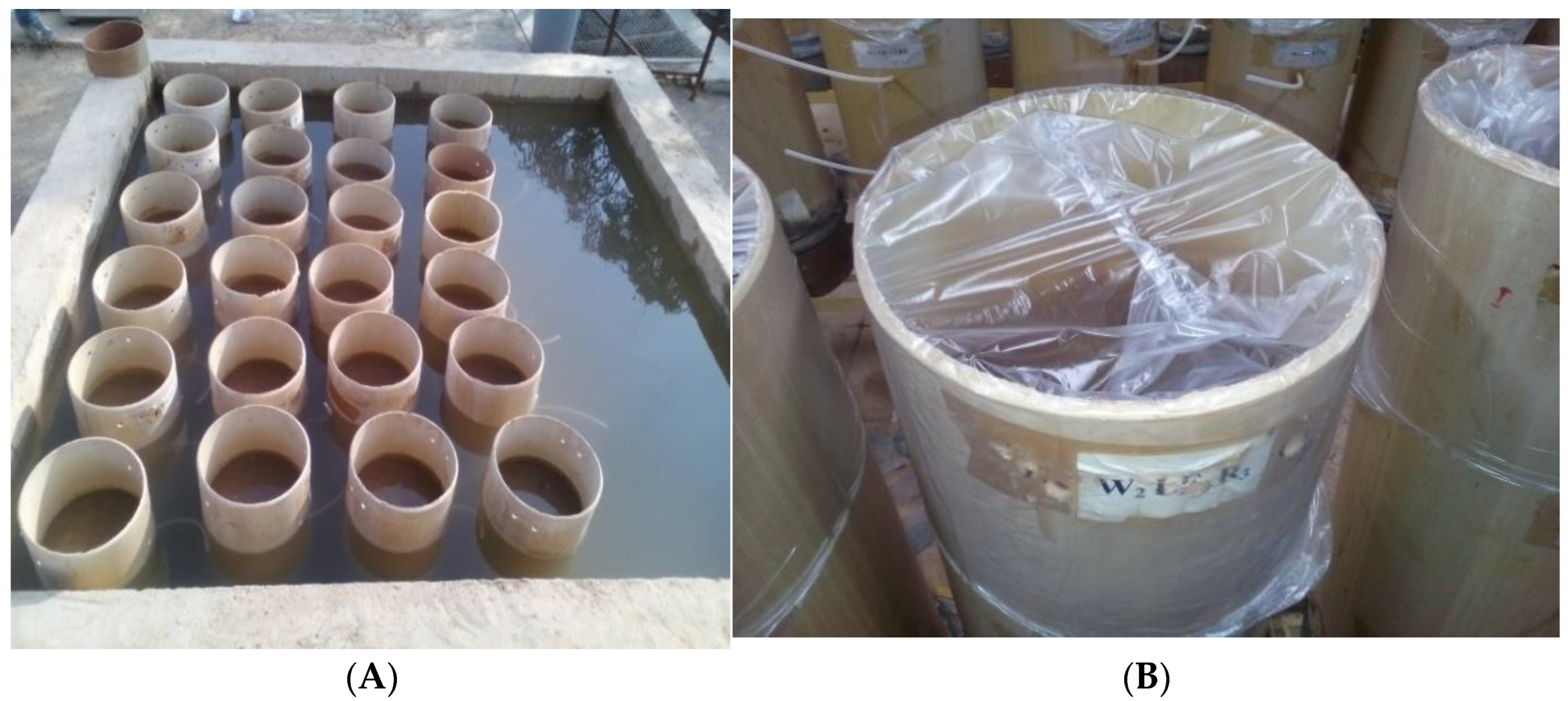
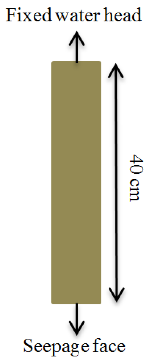
2.4. Laboratory Experiments

In the Iranian province of Isfahan, the soil samples for this study were collected from the 0–40 cm layer. PVC cylinders with a 25 cm diameter and a height of 60 cm were used to prepare the soil columns. To provide drainage, 5 cm of gravel was placed in the bottom of the columns. The top 15 cm of the column was left empty to apply irrigation water, and the soil bulk density was 1.60 g cm⁻³. The soil columns were covered in plastic to prevent evaporation after being saturated from the bottom (Figure 1). The moisture level of the soil was FC two days after saturation. Next, the cover from the columns was removed. By the weighing procedure, the soil moisture was calculated at FC. The air temperature was set at 25 °C by fans, thermostats and heaters. In all the treatments, the infiltration experiment by similar water of irrigation was conducted after 16, 56 and 114 days for I_b, I_m and I_e, respectively. The infiltration experiment was performed when the soil moisture reached 70% of field capacity. During the experiment, a 5 cm fixed water head was set in every soil using a Marriott-type bottle. When the infiltration velocity reached a steady value, the experiment was concluded. Drain water was gathered from the column outlet. Next, soil sampling was performed before the experiment in three steps at I_b, I_m and I_e.

2.5. Simulation of Infiltration Process and Sensitivity Analysis

In this article, the HYDRUS-1D model is divided into two parts. The first part is the optimization of the soil hydraulic parameters via the inverse solution. The second part is the modeling of the infiltration by the optimization of soil hydraulic parameters. The modeling of the 1D infiltration was performed via the HYDRUS-1D (v 4.16) model [24]. For the inverse solution, the van Genuchten–Mualem (1980) hydraulic model was used [25]. The van Genuchten–Mualem (1980) model parameters, including saturated moisture (θ_s [-]), saturated hydraulic conductivity (K_s [cm min⁻¹]), shape parameter (n [-]) and scaling parameter (α [cm⁻¹]) were optimized. For optimizing these parameters, the optimized soil hydraulic parameters were considered according to Javadi et al. (2019a) (

Table 4. Optimized parameters of the van Genuchten–Mualem (1980) model for all treatments.

FC	Drain Water	Infiltration	Hydraulic Parameters				Treatment
RMSE (%)	RMSE (cm)	RMSE (cm)	Ks (cm min−1)	n (-)	α (cm−1)	θs (-)
0.18	0.17	0.26	0.108	1.89	0.0119	0.200	Qg.Mi.Ib
0.06	0.13	0.19	0.097	1.48	0.0145	0.184	Qm.Mi.Ib
0.01	0.55	0.18	0.102	1.46	0.0178	0.210	Qh. Mi.Ib
0.17	0.13	0.18	0.055	1.89	0.0035	0.171	Qg.Md.Ib
0.08	0.03	0.09	0.071	1.30	0.0220	0.203	Qm.Md.Ib
0.29	0.33	0.19	0.046	1.27	0.0020	0.164	Qh.Md.Ib
1.01	0.13	0.16	0.019	1.54	0.0005	0.157	Qg.Mi.Im
0.44	0.06	0.17	0.027	1.28	0.0459	0.170	Qm.Mi.Im
0.63	0.06	0.21	0.022	1.16	0.0498	0.161	Qh.Mi.Im
0.79	3.72	1.61	0.183	2.25	0.0128	0.242	Qg.Md.Im
0.75	2.86	1.10	0.199	2.10	0.0153	0.250	Qm.Md.Im
0.73	2.17	1.06	0.198	2.37	0.0123	0.233	Qh.Md.Im
0.01	0.05	0.13	0.042	1.19	0.0644	0.179	Qg.Mi.Ie
0.26	0.05	0.11	0.026	1.17	0.0760	0.179	Qm.Mi.Ie
0.29	0.25	0.24	0.029	1.19	0.0780	0.174	Qh.Mi.Ie
0.21	0.05	0.04	0.018	1.29	0.0422	0.182	Qg.Md.Ie
0.67	0.73	0.46	0.094	1.79	0.0060	0.207	Qm.Md.Ie
0.01	0.48	0.40	0.120	1.63	0.0066	0.209	Qh.Md.Ie

θ_s is saturated moisture; n is shape parameter; α is scaling parameter; K_s is saturated hydraulic conductivity; Q_g is the low saline–sodic water quality; Q_m is the medium saline–sodic water quality; Q_h is the high saline–sodic water quality; M_i is intermittent management; M_d is daily management; I_b is an 8 day period of irrigation; I_m is a 45 day period of irrigation; I_e is a 100 day period of irrigation; and RMSE is the root mean squares of errors.

) [26]. In the research by Javadi et al. (2019a), four parameters (α, K_s, n and θ_s) were considered as uncertain parameters and soil water content at field capacity, drain water and cumulative infiltration were taken into consideration as specified parameters. Furthermore, −100 cm in field capacity was considered to be the matric potential. The Levenberg–Marquardt optimization algorithm is used by the HYDRUS-1D software for inverse estimation. Using the ROSETTA built into the HYDRUS-1D software, the initial, maximum and minimum values of θ_s, θ_r, l, K_s, α and n were calculated (

Table 5. The boundary values of the van Genuchten–Mualem parameters.

Boundary	θr (cm3cm−3)	θs (cm3cm−3)	α (cm−1)	n (-)	Ks (cm min−1)	l (-)
Initial	0.0456	0.34	0.0441	1.45	0.029	0.5
Maximum	-	0.46	0.145	2.68	1	-
Minimum	-	0.15	0.0001	1.09	0.005	-

).

The optimized parameters of any soil were used for simulating 1D infiltration. For simulating infiltration by HYDRUS-1D, the single-layer with a 40 cm depth, the lower and upper boundary conditions were given as seepage face and fixed water head, respectively (Figure 2). The fixed water heads of 2.5, 5.0, 10.0 and 20.0 cm and the four initial soil moisture between the optimized amounts of θ_r and θ_s were applied. In this study, all the boundaries were considered the same for all infiltration equations. The whole number of simulations was 288 (initial soil moisture (4) × number of pressure heads (4) × number of treatments (18)).

2.6. Infiltration Equations

In this research, the infiltration equations included: Kostiakov (Equation (1)), Kostiakov–Lewis (Equation (2)), Philip (Equation (3)), Horton (Equation (4)) and SCS (Equation (5)), which are defined as follows [27,28,29,30,31] as Equations (1)–(5):

$$\mathrm{Z}=a{\mathrm{t}}^b$$

(1)

$$\mathrm{Z}=A{\mathrm{t}}^B+f_0\mathrm{t}$$

(2)

$$\mathrm{Z}=S{\mathrm{t}}^{0.5}+k_s\mathrm{t}$$

(3)

$$\mathrm{Z}=f_f\mathrm{t}+\frac{f_i-f_f}{k}(1-{\mathrm{e}}^{-k\mathrm{t}})$$

(4)

$$\mathrm{Z}=c{\mathrm{t}}^d+0.6985$$

(5)

where Z (cm) is the cumulative infiltration; t (min) is time; a (cm min^−b), b (-), A (cm min^−B) and B (-) are the empirical coefficients; $f_0$ (cm min⁻¹) is the final infiltration capacity; S (cm min^−0.5) is the soil absorption coefficient; $k_s$ (cm min⁻¹) is the hydraulic conductivity transition zone; $f_i$ (cm min⁻¹) is the initial infiltration capacity; $f_f$ (cm min⁻¹) is the final infiltration capacity; k (min⁻¹) is the decay time constant; and c (cm min^−d) and d (-) are the empirical coefficients. Infiltration depth versus time was used to develop a differential equation using Microsoft Excel 2016 (Solver Tools). The equations were developed (i.e., their coefficients were optimized) by minimizing the root mean squares of errors (RMSE) between the fitted and measured amounts of cumulative infiltration. The RMSE were determined as Equation (6):

$$\mathrm{RMSE}=\sqrt{\left(\frac{1}{e}\sum _{i=1}^e{\left(O_i-P_i\right)}^2\right)}$$

(6)

where P_i = the calculated amount, O_i = the measured amount, and e = the amount of data.

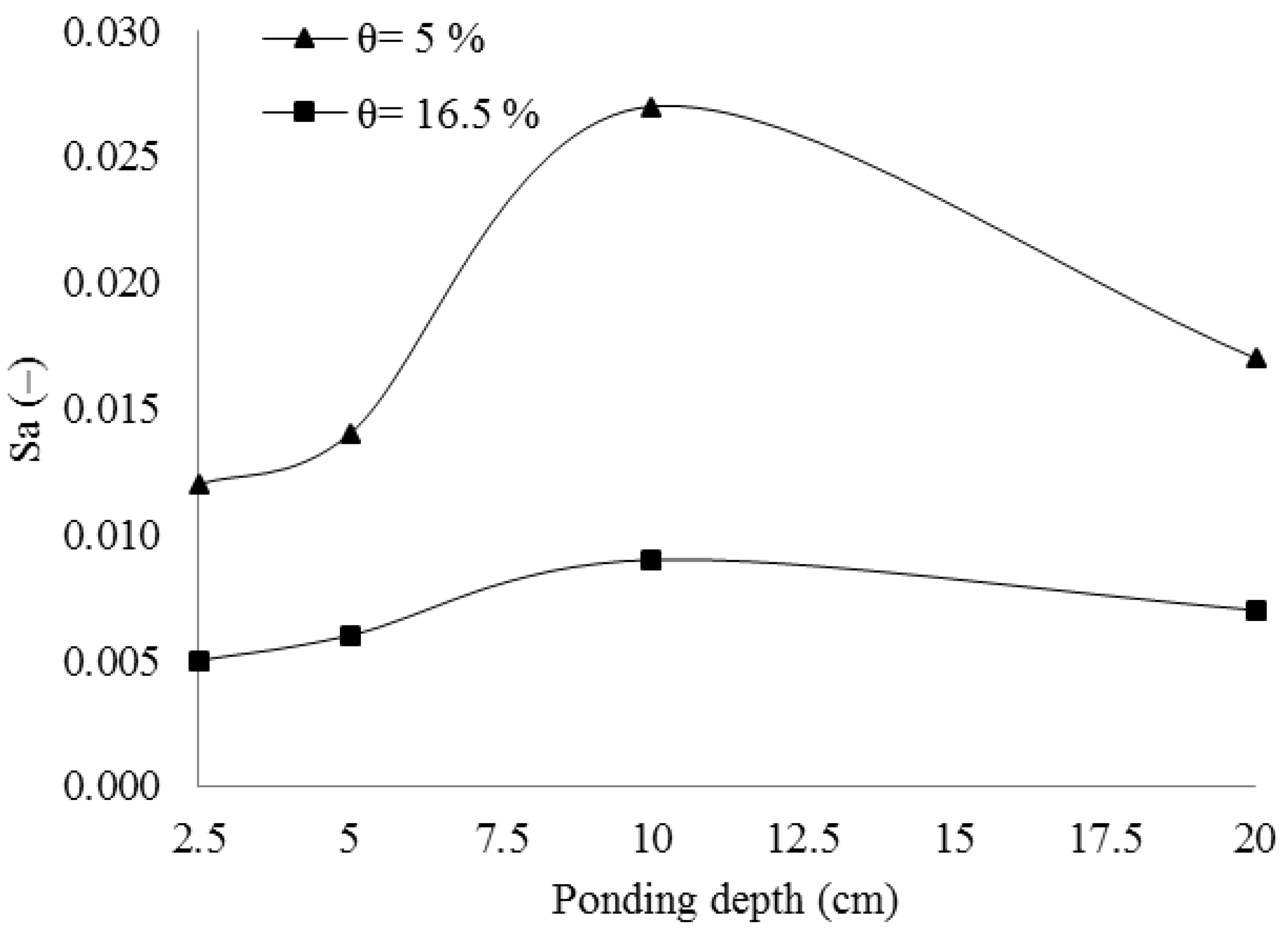
2.7. Sensitivity Analysis

The sensitivities of the infiltration equations and their coefficients were investigated by the relative and absolute sensitivity indicators. The analysis of sensitivity was performed under two conditions. In the first condition, the water head was fixed and the initial soil moisture was varied. For example, four simulations were carried out for the initial soil moistures of 0.05, 0.10, 0.15 and 0.20 while the constant ponding depth was fixed at 5 cm. In the second condition, the ponding depth was varied, but the initial soil moisture was fixed. The absolute and relative sensitivity indicators were defined by the following equations (Javadi et al., 2019a) as Equations (7) and (8):

$${\mathrm{S}}_{\mathrm{r}}=\frac{1}{m}{\sum }_{\mathrm{i}=1}^m\frac{\frac{X_i-X_{i-1}}{\frac{X_i+X_{i-1}}{2}}}{\frac{P_i-P_{i-1}}{\frac{P_i+P_{i-1}}{2}}}$$

(7)

$${\mathrm{S}}_{\mathrm{a}}=\frac{1}{m}{\sum }_{\mathrm{i}=1}^m\left|\frac{\frac{X_i-X_{i-1}}{\frac{X_i+X_{i-1}}{2}}}{\frac{P_i-P_{i-1}}{\frac{P_i+P_{i-1}}{2}}}\right|$$

(8)

where m is the number of outputs; X_i is the new output, as a result of varying the input from P_i−1 to P_i; X_i−1 is the prior output, without varying the input (P_i−1); S_r is the relative sensitivity indicator (dimensionless); and S_a is the absolute sensitivity indicator (dimensionless) [26]. Each infiltration equation (or coefficient) indicator near to zero has less sensitivity. For every treatment under the given irrigation period, the sensitivity indicators for the first condition (the initial soil moisture (ϴ) was increased and the ponding depth (H) was constant (C); i.e., H = c, ϴ ↑) were calculated with four constant ponding depths using Equations (7) and (8). The averages of the indicators are shown by the symbols mS_a and mS_r for the absolute and relative sensitivity indicators analysis, respectively. The same procedure was repeated for the same treatment in other irrigation periods. The calculated averages of mS_a (mS_r) for the three irrigation periods are shown by MS_a (or MS_r). The same procedures were applied to the second condition (ϴ = c, H ↑). By using the above-mentioned procedure, the trends in changes in the infiltration equations (or coefficients) could be followed. If the differences between the absolute and relative values were equal to zero, it would mean that the changes were quite systematic. In this study, for the infiltration equations and their coefficients sensitivity analysis, the ranking method based on MS_a was used. For each condition, the ranking and comparison were performed for all of the treatments. Any equation (or coefficient) with the lowest ranking in both conditions was introduced as the least sensitive equation (or coefficient). Finally, any equation (or coefficient) that had the lowest ranking in six treatments was introduced as the least sensitive equation (or coefficient).

3. Results and Discussion

3.1. Experimental Columns

The chemical properties of the studied soil, before the infiltration tests and cumulative infiltration, are given in

Table 6. Chemical characteristics of the soil before infiltration experiments and cumulative infiltration.

Cumulative Infiltration (cm, at 100 min)	SARe (meq·L−1)−0.5	ECe (dS m−1)	Treatments
13.7	0.72	1.05	Qg.Mi.Ib
12.3	2.61	1.27	Qm.Mi.Ib
12.8	2.29	1.96	Qh.Mi.Ib
8.3	1.74	1.21	Qg.Md.Ib
9.3	2.22	1.74	Qm.Md.Ib
7.6	4.64	1.88	Qh.Md.Ib
4.6	1.77	1.32	Qg.Mi.Im
4.1	3.77	2.63	Qm.Mi.Im
4.2	6.21	4.88	Qh.Mi.Im
23.6	1.99	1.08	Qg.Md.Im
25.5	5.93	3.42	Qm.Md.Im
25.3	5.65	4.58	Qh.Md.Im
5.7	1.33	1.32	Qg.Mi.Ie
3.7	6.06	3.44	Qm.Mi.Ie
4.2	10.36	6.35	Qh.Mi.Ie
3.0	1.81	1.35	Qg.Md.Ie
13.4	7.37	4.78	Qm.Md.Ie
16.2	14.42	8.12	Qh.Md.Ie

Q_g is the low saline–sodic water quality; Q_m is the medium saline–sodic water quality; Q_h is the high saline–sodic water quality; M_i is intermittent management; M_d is daily management; I_b is an 8 day period of irrigation; I_m is a 45 day period of irrigation and I_e is a 100 day period of irrigation.

. Moreover, the coefficients of the infiltration equations are presented in

Table 7. Infiltration equation coefficients for all treatments.

Infiltration Equation Coefficients												Treatment
SCS		Philip		Horton			Kostiakov–Lewis			Kostiakov
d	c	${\mathit{k}}_{\mathit{s}}$	S	ff	fi	k	f0	B	A	b	a
0.810	0.315	0.081	0.588	0.123	0.637	0.275	0.108	0.925	0.275	0.458	0.740	Qg.Mi.Ib
0.832	0.202	0.055	0.453	0.089	1.076	0.724	0.100	0.765	0.265	0.354	0.725	Qm.Mi.Ib
0.876	0.183	0.070	0.405	0.100	1.306	0.994	0.106	0.727	0.275	0.315	0.770	Qh.Mi.Ib
0.628	0.498	0.017	0.810	0.078	3.191	1.287	0.060	1.365	0.163	0.782	0.546	Qg.Md.Ib
0.791	0.204	0.038	0.471	0.073	0.790	0.500	0.077	0.650	0.221	0.381	0.673	Qm.Md.Ib
0.746	0.278	0.037	0.573	0.080	2.584	1.463	0.057	1.289	0.122	0.479	0.645	Qh.Md.Ib
0.632	0.167	0.022	0.206	0.027	1.295	0.993	0.021	1.257	0.150	0.510	0.430	Qg.Mi.Im
0.963	0.060	0.032	0.251	0.050	0.603	0.731	0.033	0.168	0.331	0.196	0.729	Qm.Mi.Im
1.365	0.006	0.028	0.089	0.034	0.117	0.296	0.024	0.049	0.652	0.076	0.841	Qh.Mi.Im
0.606	1.359	0.060	1.735	0.190	3.359	0.604	0.165	3.435	0.167	1.565	0.585	Qg.Md.Im
0.526	1.738	0.058	1.675	0.158	4.560	0.746	0.183	4.302	0.119	2.035	0.502	Qm.Md.Im
0.610	1.301	0.061	1.677	0.186	3.064	0.566	0.189	2.724	0.190	1.503	0.589	Qh.Md.Im
0.975	0.059	0.034	0.246	0.052	0.987	1.273	0.049	0.529	0.090	0.191	0.740	Qg.Mi.Ie
1.281	0.010	0.029	0.107	0.037	0.333	0.917	0.033	0.287	0.089	0.088	0.827	Qm.Mi.Ie
1.068	0.033	0.032	0.186	0.046	0.408	0.645	0.039	0.120	0.133	0.145	0.769	Qh.Mi.Ie
0.922	0.050	0.014	0.267	0.034	0.783	0.936	0.022	0.415	0.128	0.229	0.622	Qg.Md.Ie
0.666	0.497	0.034	0.817	0.095	1.858	0.717	0.091	1.327	0.257	0.721	0.600	Qm.Md.Ie
0.716	0.450	0.053	0.771	0.111	1.401	0.551	0.121	1.169	0.268	0.636	0.653	Qh.Md.Ie

Q_g is the low saline–sodic water quality; Q_m is the medium saline–sodic water quality; Q_h is the high saline–sodic water quality; M_i is intermittent management; M_d is daily management; I_b is an 8 day period of irrigation; I_m is a 45 day period of irrigation and I_e is a 100 day period of irrigation.

. At the beginning of the period, the period irrigation and management had little effect on the amount of infiltration. With the rising irrigation period, as compared to the beginning, the cumulative infiltration in the intermittent management was decreased. A soil crust that could remarkably decrease the infiltration rate was seen only in intermittent management. Therefore, infiltrations under the intermittent management were less than that under the daily management. Raising the SAR/EC of the water and soil under the intermittent management led to soil particle dispersion, consequently reducing the infiltration rate. Readers can refer to Javadi et al. (2019b) for further information on the effects of the three treatments on soil chemical and physical characteristics [32]. According to

Table 8. Error values of infiltration equations in estimating measured infiltration.

RMSE (cm)					Treatment
SCS	Philip	Horton	Kostiakov–Lewis	Kostiakov
0.148	0.175	0.035	0.079	0.236	Qg.Mi.Ib
0.096	0.106	0.031	0.053	0.176	Qm.Mi.Ib
0.099	0.108	0.040	0.057	0.183	Qh.Mi.Ib
0.153	0.238	0.03	0.104	0.219	Qg.Md.Ib
0.071	0.064	0.044	0.035	0.118	Qm.Md.Ib
0.118	0.181	0.033	0.089	0.166	Qh.Md.Ib
0.128	0.296	0.057	0.107	0.131	Qg.Mi.Im
0.075	0.029	0.022	0.012	0.055	Qm.Mi.Im
0.108	0.017	0.026	0.009	0.045	Qh.Mi.Im
0.555	0.507	0.026	0.138	0.677	Qg.Md.Im
0.606	0.546	0.028	0.151	0.726	Qm.Md.Im
0.448	0.345	0.217	0.269	0.474	Qh.Md.Im
0.080	0.041	0.032	0.022	0.086	Qg.Mi.Ie
0.098	0.019	0.028	0.010	0.051	Qm.Mi.Ie
0.090	0.023	0.029	0.012	0.056	Qh.Mi.Ie
0.100	0.017	0.033	0.006	0.041	Qg.Md.Ie
0.272	0.283	0.032	0.115	0.379	Qm.Md.Ie
0.284	0.285	0.029	0.105	0.404	Qh.Md.Ie

Q_g is the low saline–sodic water quality; Q_m is the medium saline–sodic water quality; Q_h is the high saline–sodic water quality; M_i is intermittent management; M_d is daily management; I_b is an 8 day period of irrigation; I_m is a 45 day period of irrigation and I_e is a 100 day period of irrigation.

, RSME values show that Horton and Kostiakov–Lewis had the lowest error and Kostiakov and SCS had the highest error in infiltration estimation. Evaluating the performance of infiltration equations using statistical indicators by various researchers showed that the Horton and Kostiakov–Lewis equations were the best equations [33,34]. One of the reasons for the superiority of the experimental equations of infiltration (Kostiakov–Lewis and Horton) was that their coefficients were higher than other equations. This feature made these equations more flexible when determining the coefficients. In the foundation of physical equations such as Philip, some limitations include creating a boundary and initial conditions to solve the Richards equation and assuming the soil to be homogeneous, which is not compatible with natural conditions, but in the foundation of experimental equations, such limitations are not applied. The aim of deriving empirical equations is to fit the infiltration data in the best way.

3.2. Simulation and Sensitivity Analysis of 1D Infiltration

3.2.1. Sensitivity Analysis of Infiltration Equations Coefficients

The values related to the MS_r and MS_a of the infiltration coefficients are presented in

Table 9. The mean sensitivity indicators of infiltration equation coefficients.

Infiltration Equation Coefficients												Sensitivity Indicator		Treatment
SCS		Philip		Horton			Kostiakov–Lewis			Kostiakov
d	c	${\mathit{k}}_{\mathit{s}}$	S	ff	fi	k	f0	B	A	b	a
0.51	−2.01	0.42	−1.26	0.00	−0.13	1.40	0.89	−1.11	−0.82	0.39	−0.70	H = c ϴ ↑	MSr (-)	QgMi
0.01	0.14	0.24	0.07	0.17	0.20	0.17	0.47	−0.13	0.14	0.03	0.05	H ↑ ϴ = c
0.51	2.02	0.42	1.27	0.02	0.14	1.41	0.90	1.12	0.83	0.40	1.47	H = c ϴ ↑	MSa (-)
0.04	0.17	0.25	0.08	0.17	0.21	0.18	0.48	0.16	0.16	0.04	0.11	H ↑ ϴ = c
2	8	6	4	3	4	7	7	5	4	1	6	Rank
0.32	−1.69	0.36	−1.28	−0.05	−0.22	1.13	0.30	−0.95	−0.69	0.25	−1.13	H = c ϴ ↑	MSr (-)	QmMi
−0.05	0.44	0.11	0.20	0.16	0.31	0.18	0.17	−0.15	0.30	−0.01	0.22	H ↑ ϴ = c
0.32	1.69	0.37	1.28	0.05	0.22	1.16	0.33	0.98	0.70	0.26	1.14	H = c ϴ ↑	MSa (-)
0.06	0.44	0.13	0.21	0.16	0.31	0.22	0.19	0.18	0.30	0.03	0.22	H ↑ ϴ = c
3	9	4	8	2	6	8	5	6	7	1	8	Rank
0.33	−1.78	0.38	−1.31	−0.05	−0.23	1.21	0.34	−0.96	−0.69	0.26	−1.18	H = c ϴ ↑	MSr (-)	QhMi
−0.06	0.51	0.12	0.20	0.16	0.30	0.17	0.17	−0.16	0.31	−0.01	0.21	H ↑ ϴ = c
0.34	1.79	0.38	1.32	0.05	0.24	1.22	0.34	0.99	0.70	0.27	1.19	H = c ϴ ↑	MSa (-)
0.07	0.52	0.13	0.21	0.16	0.32	0.24	0.19	0.18	0.31	0.03	0.22	H ↑ ϴ = c
3	10	4	8	2	6	9	5	6	7	1	7	Rank
0.48	−2.07	1.20	−1.32	−0.05	−0.31	1.06	0.32	−1.21	−1.00	0.39	−1.46	H = c ϴ ↑	MSr (-)	QgMd
−0.01	0.24	0.23	0.09	0.16	0.14	0.07	0.16	−0.07	0.09	0.03	0.08	H ↑ ϴ = c
0.49	2.08	1.20	1.32	0.05	0.32	1.13	0.36	1.26	1.00	0.40	1.47	H = c ϴ ↑	MSa (-)
0.07	0.30	0.45	0.11	0.16	0.14	0.13	0.19	0.11	0.10	0.06	0.14	H ↑ ϴ = c
2	9	8	6	4	3	5	5	5	3	1	7	Rank
0.33	−1.46	0.58	−1.36	0.00	−0.16	1.25	0.19	−1.33	−0.96	0.31	−1.26	H = c ϴ ↑	MSr (-)	QmMd
0.02	0.08	0.25	0.03	0.17	0.16	0.14	0.20	−0.14	0.09	0.03	0.03	H ↑ ϴ = c
0.33	1.46	0.59	1.37	0.01	0.17	1.26	0.19	1.34	0.96	0.31	1.26	H = c ϴ ↑	MSa (-)
0.03	0.12	0.26	0.06	0.17	0.16	0.15	0.20	0.15	0.09	0.04	0.09	H ↑ ϴ = c
1	8	8	6	3	3	2	6	7	4	1	5	Rank
0.48	−1.89	1.52	−1.42	0.00	−0.15	1.41	0.78	−1.30	−0.89	0.42	−1.57	H = c ϴ ↑	MSr (-)	QhMd
0.05	0.01	0.25	0.00	0.13	0.09	0.11	0.23	−0.09	0.03	0.04	−0.02	H ↑ ϴ = c
0.48	1.89	1.52	1.43	0.00	0.16	1.42	0.79	1.31	0.90	0.43	1.58	H = c ϴ ↑	MSa (-)
0.05	0.09	0.48	0.02	0.13	0.10	0.11	0.39	0.11	0.05	0.04	0.04	H ↑ ϴ = c
2	9	10	3	4	2	8	7	6	3	1	5	Rank
2	10	9	6	3	4	8	6	6	5	1	7	Final ranking

(H = c, ϴ ↑): the initial soil moisture was raised, and the ponding depth was fixed; (ϴ = c, H ↑): the ponding depth was raised, and the initial soil moisture was fixed; MS_r: the relative sensitivity indicator; MS_a: the absolute sensitivity indicator; Q_g: low saline–sodic water quality; Q_m: medium saline–sodic water quality; Q_h: high saline–sodic water quality; M_i: intermittent management and M_d: daily management.

, showing that small differences between the values of MS_r and MS_a represent systematic changes in the coefficients of the infiltration equations. The values of MS_r under the first condition (H = c, ϴ ↑) indicated that the change in a, A, B, f_f, S, c had decreasing trends, whereas under the second condition (ϴ = c, H ↑), the change in the coefficients had an increasing trend, except for the B. The reason for these changes was the nature of the coefficients. Some coefficients have an empirical nature (i.e., a, b), while others have some physical nature (i.e., k_s, S). Therefore, the infiltration coefficients change according to their nature. The values of MS_a showed that the coefficients of the infiltration equations under the first condition (H = c, ϴ ↑) were much more sensitive compared to the second condition (ϴ = c, H ↑). Based on the Darcy equation (q = K·i), in the infiltration process, ponding depth influences only the hydraulic gradient (i), but the initial soil moisture affects both the hydraulic gradient and hydraulic conductivity (K). Therefore, significant changes in the coefficients of an infiltration equation due to varying initial moisture content occurred owing to the influences on both driving forces and the conductance of soil. For the same water quality of the first condition (H = c, ϴ ↑), the sensitivities were greater for the daily management than that one. For the same water quality in the second condition (ϴ = c, H ↑), the sensitivities were greater for the intermittent management than for the daily management. The results indicated that the effect of initial soil moisture variations on the infiltration coefficients in the high permeable soil (arising from the daily management) was higher, but in low permeable soil (arising from the intermittent management), the ponding depth changes were more effective. One of the reasons for increasing the sensitivity with respect to the initial soil moisture under daily management is that by changing the initial soil moisture, the capacity of water holding in this management is more significantly increased than that one. Therefore, the initial soil moisture variations in the simulations were larger in the daily management, and this led to a greater change in the coefficients and cumulative infiltration. Under the intermittent management, the initial soil moisture variations were smaller. Thus, the effects of varying ponding depth on the infiltration changes (coefficients) were larger in this management compared to the initial soil moisture changes. Sensitivity was incremented by raising EC and SAR of irrigation water and soil solution quality under the daily management and the first condition (H = c, ϴ ↑). Under the second condition (ϴ = c, H ↑), the sensitivity was decreased, whereas in the intermittent management, there was an inverse behavior. The results of various studies indicated that water quality could affect infiltration [6]. In general, the effect of irrigation management treatment on the sensitivity of the coefficients was higher compared to the irrigation water quality treatment. The coefficient b in the Kostiakov equation, with the average absolute sensitivity indicator of all simulated cases with a value of 0.19, had the smallest ranks and was the least sensitive. The coefficient c in the SCS equation, with the average absolute sensitivity indicator of all simulated cases with a value of 1.05, had the highest rank and was the most sensitive. The high sensitivity of the coefficient c in the SCS equation showed that it depended on the soil intrinsic characteristics, soil moisture and ponding depth. The least sensitive coefficient of b in the Kostiakov equation showed that it depended on only the intrinsic properties of soil, in comparison to the changes in the environmental characteristics. Our results are partially in agreement with the results obtained by other researchers such as Turner (2006), Javadi et al. (2014) and Hoyos and Cavalcante (2015) [15,16,17]. For example, Hoyos and Cavalcante (2015) showed that the exponent of the Kostiakov equation was a less sensitive coefficient, showing agreement with our results. However, Turner (2006) showed that the final intake rate of the Horton equation was a more sensitive coefficient, which was not in line with our results. One of the reasons for these different results is the variable nature of the infiltration process, so that the performance of an infiltration equation would vary even in two soils with apparently similar physical properties [35,36]. Furthermore, the different methods of measuring the infiltration and the boundary and initial conditions of soil water flow can affect the results [37].

3.2.2. Sensitivity Analysis of Infiltration Equations

The changes in the sensitivity of different equations related to the initial soil moisture and ponding depth were similar, as seen in Figure 3. Figure 3 shows that the infiltration equations are more sensitive to low initial soil moisture and high ponding depth since the infiltration capacity of soil increased under low soil moisture and high ponding depth. The values of MS_r and MS_a related to the infiltration equations are presented in

Table 10. The mean sensitivity indicators of infiltration equations.

Infiltration Equations					Sensitivity Indicator		Treatment
SCS	Philip	Horton	Kostiakov–Lewis	Kostiakov
−0.290	−0.348	−0.306	−0.300	−0.305	H = c, ϴ ↑	MSr(-)	QgMi
0.136	0.138	0.139	0.139	0.137	ϴ = c, H ↑
0.290	0.348	0.306	0.300	0.305	H = c, ϴ ↑	MSa(-)
0.136	0.138	0.139	0.139	0.137	ϴ = c, H ↑
1	4	5	3	2	Rank
−0.179	−0.194	−0.200	−0.192	−0.188	H = c, ϴ ↑	MSr(-)	QmMi
0.163	0.167	0.168	0.168	0.167	ϴ = c, H ↑
0.179	0.194	0.200	0.192	0.188	H = c, ϴ ↑	MSa(-)
0.163	0.167	0.168	0.168	0.167	ϴ = c, H ↑
1	3	5	4	2	Rank
−0.185	−0.199	−0.206	−0.197	−0.191	H = c, ϴ ↑	MSr(-)	QhMi
0.161	0.167	0.167	0.168	0.168	ϴ = c, H ↑
0.185	0.199	0.206	0.197	0.191	H = c, ϴ ↑	MSa(-)
0.161	0.167	0.167	0.168	0.168	ϴ = c, H ↑
1	2	3	3	2	Rank
−0.239	−0.264	−0.270	−0.259	−0.251	H = c, ϴ ↑	MSr(-)	QgMd
0.149	0.148	0.150	0.151	0.152	ϴ = c, H ↑
0.239	0.264	0.270	0.259	0.251	H = c, ϴ ↑	MSa(-)
0.149	0.148	0.150	0.151	0.152	ϴ = c, H ↑
1	2	4	4	3	Rank
−0.140	−0.150	−0.165	−0.158	−0.143	H = c, ϴ ↑	MSr(-)	QmMd
0.152	0.153	0.151	0.152	0.153	ϴ = c, H ↑
0.140	0.150	0.165	0.158	0.143	H = c, ϴ ↑	MSa(-)
0.152	0.153	0.151	0.152	0.153	ϴ = c, H ↑
1	3	2	3	3	Rank
−0.247	-0−264	−0.268	−0.256	−0.254	H = c, ϴ ↑	MSr(-)	QhMd
0.106	0.105	0.107	0.107	0.107	ϴ = c, H ↑
0.247	0.264	0.268	0.256	0.254	H = c, ϴ ↑	MSa(-)
0.106	0.105	0.107	0.107	0.107	ϴ = c, H ↑
1	2	5	4	3	Rank
1	3	5	4	2	Final ranking

(H = c, ϴ ↑): the initial soil moisture was raised, and the ponding depth was fixed; (ϴ = c, H ↑): the ponding depth was raised, and the initial soil moisture was fixed; MS_r: the relative sensitivity indicator; MS_a: the absolute sensitivity indicator; Q_g: low saline–sodic water quality; Q_m: medium saline–sodic water quality; Q_h: high saline–sodic water quality; M_i: intermittent management and M_d: daily management.

. The values of MS_a showed that in all the infiltration equations, for the first condition (H = c, ϴ ↑), the changes were higher when compared to the second condition (ϴ = c, H ↑). The reason for the first condition (H = c, ϴ ↑) was that by raising the initial soil moisture, the matric suction was reduced (Liu et al. 2011) [38]. In the second condition (ϴ = c, H ↑), by increasing the ponding depth, the hydraulic gradient was raised [39]. Given the lack of difference between the absolute and relative sensitivity indicators, all the infiltration equations had systematic changes. These results indicate that the infiltration rate increased with the increasing hydraulic gradient and hydraulic conductivity of the infiltrating soil profile (i.e., increasing ponding depth and decreasing initial soil moisture).

For similar coefficients, the values of the MS_a indicator showed that all the infiltration equations in the first condition (H = c, ϴ ↑) were more sensitive in comparison with those in the second condition (ϴ = c, H ↑). The effects of poor water quality and soil solution on the structure of soil in the intermittent management and the first condition (H = c, ϴ ↑) showed that the sensitivity was decreased. In the second condition (ϴ = c, H ↑), the sensitivity was increased. The results of various studies indicated that high EC-SAR in the water quality could cause the soil crust formation [40,41]. The effect of management and increasing the EC-SAR of the water quality and soil solution on the sensitivity of the infiltration equations was similar to the sensitivity of the coefficients. In our study, the infiltration rate decreased with the increasing EC and SAR of water and soil. As previously noted, the effect of the initial soil moisture on the infiltration rate in low permeable soil was less, but the ponding depth was effective. In the first condition (H = c, ϴ ↑) and for the daily management with medium irrigation water quality, the sensitivity was the lowest. In the second condition (ϴ = c, H ↑), the sensitivity was decreased. The daily management with daily leaching led to a reduction in the harmful effects of sodium, and the salinity of the water and soil increased the infiltration [10]. Similar to the analysis of the sensitivity coefficients, the effect of ponding depth on the infiltration changes decreased with increasing soil infiltration rate.

The results revealed that the Horton equation with the average absolute sensitivity indicator of all simulated cases with a value of 0.191 was the most sensitive one. The SCS equation with the average absolute sensitivity indicator of all simulated cases with a value of 0.179 was the least sensitive one. One of the reasons for the high sensitivity of the Kostiakov–Lewis and Horton equations was the higher number of their coefficients. This feature made these models more flexible during fitting. The results also indicated that the Horton and Kostiakov–Lewis equations changed significantly with the initial soil moisture and ponding depth changes so that cumulative infiltration could be easily estimated.

4. Conclusions

In this study, infiltration experiments were performed under two irrigation management systems. Then, the laboratory model of infiltration was calibrated with the HYDRUS-1D model. Next, the HYDRUS-1D model was used for simulating infiltration in various initial soil moistures and ponding depths under different irrigation management. The initial soil moisture had a greater effect on the changes in infiltration coefficients due to the simultaneous effect on both driving forces and the conductance of soil. The process of wetting and drying of the soil, which caused a soil surface strength in the M_d soil moisture management, was also one of the important factors in the difference between the two managements. Evaluating the performance of infiltration equations via RMSE indicator showed that the results from the infiltration empirical equations (Kostiakov–Lewis and Horton) were closer to the actual values than other cumulative infiltrations under various initial and boundary conditions. Irrigation management and irrigation duration were found to be much more effective on cumulative infiltration during the wetting and drying periods, while irrigation water quality had a minor effect. Infiltration in the daily management was higher than in intermittent management because the intermittent management caused the soil seal formation. The results indicated that the effect of initial soil moisture changes on the coefficients of the infiltration equations in soil with high permeability (arising from the daily management) was greater; but in low permeable soil (arising from the intermittent management), the ponding depth changes were more effective. The infiltration equations were more sensitive to low soil moisture and high ponding depth. Therefore, with increasing irrigation period and inflow rate (ponding depth) to the field, the sensitivity of the infiltration equation is increased. For a specific irrigation management, poor irrigation water and soil solution quality in the intermittent and daily managements reduced and increased infiltration, respectively. Sensitivity was incremented with the increasing SAR and EC of soil and irrigation water in daily management and the first condition (H = c, ϴ ↑). In the second condition (ϴ = c, H ↑), the sensitivity was decreased, while there was an inverse behavior in intermittent management. According to the results of this research, it is suggested that the infiltration equations (specifically SCS equation) and their coefficients (specifically coefficient c) should be calibrated relative to the initial soil moisture, ponding depth, soil solution and water irrigation quality. Particularly in areas with high permeable soil (in the daily management), the calibration of the infiltration equation should be implemented with the initial soil moisture. In these areas, the irrigation period should be controlled. In areas with low permeable soil (in the intermittent management), the calibration should be carried out relative to the ponding depth. In these areas, the inflow rate should be controlled. It is also recommended to use the Horton equation, which had the highest sensitivity to the initial soil moisture and inlet ponding depth changes. Surface irrigation is mostly conducted in soils with a medium texture. In this research, medium texture (sandy loam) was used so that the results of this research, which are close to the conditions of most surface irrigation soil textures, can be used. Further work is needed to be carried out under field conditions for various surface irrigation systems to validate the results of the column study.

References

1. Chari, M.M.; Poozan, M.T.; Afrasiab, P. Modeling infiltration in surface irrigation with minimum measurement (study of USDA–NRCS intake families). Model. Earth Syst. Environ. 2021, 7, 433–441. [Google Scholar] [CrossRef]
2. Javadi, A.; Shayannejad, M.; Ebrahimian, H.; Ghorbani-Dashtaki, S. Simulation modeling of border irrigation performance under different soil texture classes and land uses. Model. Earth Syst. Environ. 2022, 8, 1135–1144. [Google Scholar] [CrossRef]
3. Moravejalahkami, B. Methods of infiltration estimation for furrow irrigation. Irrig. Drain. 2019, 69, 52–62. [Google Scholar] [CrossRef]
4. Babaei, F.; Zolfaghari, A.A.; Yazdani, M.R.; Sadeghipour, A. Spatial analysis of infiltration in agricultural lands in arid areas of Iran. Catena 2018, 170, 25–35. [Google Scholar] [CrossRef]
5. Rezaei, M.; Seuntjens, P.; Shahidi, R.; Joris, I.; Boënne, W.; Al-Barri, B.; Cornelis, W. The relevance of in-situ and laboratory characterization of sandy soil hydraulic properties for soil water simulations. J. Hydrol. 2016, 534, 251–265. [Google Scholar] [CrossRef]
6. Emdad, M.R.; Raine, S.R.; Smith, R.J.; Fardad, H. Effect of water quality on soil structure and infiltration under furrow irrigation. Irrig. Sci. 2004, 23, 55–60. [Google Scholar] [CrossRef]
7. Choudhary, O.P.; Ghuman, B.S.; Josan, A.S.; Bajwa, M.S. Effect of alternating irrigation with sodic and non-sodic waters on soil properties and sunflower yield. Agric. Water Manag. 2006, 85, 151–156. [Google Scholar] [CrossRef]
8. Feki, M.; Ravazzani, G.; Ceppi, A.; Milleo, G.; Mancini, M. Impact of infiltration process modeling on soil water content simulations for irrigation management. Water 2018, 10, 850. [Google Scholar] [CrossRef]
9. Rocha, D.; Abbasi, F.; Feyen, J. Sensitivity analysis of soil hydraulic properties on subsurface water flow in furrows. J. Irrig. Drain. Eng. 2006, 132, 418–424. [Google Scholar] [CrossRef]
10. Malik, M.; Mustafa, M.A.; Letey, J. Effect of mixed Na/Ca solutions on swelling, dispersion and transient water flow in unsaturated montmorillonitic soils. Geoderma 1992, 52, 17–28. [Google Scholar] [CrossRef]
11. Al-Darby, A.M.; Mustafa, M.A.; Al-Omran, A.M. Effect of water quality on infiltration of loamy sand soil treated with three gel-conditioners. Soil Technol. 1990, 3, 83–90. [Google Scholar] [CrossRef]
12. Sepaskhah, A.R.; Afshar-Chamanabad, H. SW-Soil and Water: Determination of Infiltration Rate for Every-other Furrow Irrigation. Biosyst. Eng. 2002, 82, 479–484. [Google Scholar] [CrossRef]
13. Shukla, M.K.; Lal, R.; Owens, L.B.; Unkefer, P. Land use and management impacts on structure and infiltration characteristics of soils in the North Appalachian region of Ohio. Soil Sci. 2003, 168, 167–177. [Google Scholar] [CrossRef]
14. Dagadu, J.S.; Nimbalkar, P.T. Infiltration studies of different soils under different soil conditions and comparison of infiltration models with field data. Int. J. Adv. Eng. Technol. 2012, 3, 154–157. [Google Scholar]
15. Turner, E.R. Comparison of Infiltration Equations and Their Field Validation with Rainfall Simulation. Master’s Thesis, Faculty of the Graduate School of the University of Maryland, College Park, MD, USA, 2006; 185p. [Google Scholar]
16. Javadi, A.; Mashal, M.; Ebrahimian, H. Sensitivity Analysis of Different Infiltration Equations and Their Coefficients under Various Initial Soil Moisture and Ponding Depth. Iran. J. Water Soil 2014, 28, 899–908. (In Persian) [Google Scholar]
17. Hoyos, E.M.; Cavalcante, A.L.B. Sensitivity Analysis of One-Dimensional Infiltration Models. Electron. J. Geotech. Eng. 2015, 20, 4313–4324. [Google Scholar]
18. Sepah Vand, A.; Sihag, P.; Singh, B.; Zand, M. Comparative evaluation of infiltration models. KSCE J. Civ. Eng. 2018, 22, 4173–4184. [Google Scholar] [CrossRef]
19. Machiwal, D.; Jha, M.K.; Mal, B.C. Modelling infiltration and quantifying spatial soil variability in a wasteland of Kharagpur, India. Biosyst. Eng. 2006, 95, 569–582. [Google Scholar] [CrossRef]
20. Asgarzadeh, H.; Mosaddeghi, M.R.; Dexter, A.R.; Mahboubi, A.A.; Neyshabouri, M.R. Determination of soil available water for plants: Consistency between laboratory and field measurements. Geoderma 2014, 226–227, 8–20. [Google Scholar] [CrossRef]
21. Ramos, T.B.; Goncalves, M.C.; Martins, J.C.; Van Genuchten, M.T.; Pires, F.P. Estimation of soil hydraulic properties from numerical inversion of tension disk infiltrometer data. Vadose Zone J. 2006, 5, 684–696. [Google Scholar] [CrossRef]
22. Mashayekhi, P.; Ghorbani-Dashtaki, S.; Mosaddeghi, M.R.; Shirani, H.; Nodoushan, A.R. Different scenarios for inverse estimation of soil hydraulic parameters from double-ring infiltrometer data using HYDRUS-2D/3D. Int. Agrophys. 2016, 30, 203–210. [Google Scholar] [CrossRef]
23. Zheng, C.; Lu, Y.; Guo, X.; Li, H.; Sai, J.; Liu, X. Application of HYDRUS-1D model for research on irrigation infiltration characteristics in arid oasis of northwest China. Environ. Earth Sci. 2017, 76, 785. [Google Scholar] [CrossRef]
24. Šimůnek, J.; van Genuchten, M.T.; Šejna, M. The HYDRUS-1D software package for simulating the one-dimensional movement of water, heat, and multiple solutes in variably-saturated media. In Technical Manual; Version 4.17; Department of Environmental Sciences, University of California at Riverside: Riverside, CA, USA, 2013; 342p. [Google Scholar]
25. Van Genuchten, M.T. A closed-form equation for predicting the hydraulic conductivity of unsaturated soils. Soil Sci. Soc. Am. J. 1980, 44, 892–898. [Google Scholar] [CrossRef]
26. Javadi, A.; Mostafazadeh-Fard, B.; Shayannejad, M.; Ebrahimian, H. Effect of Initial Soil Water Content on Output Parameters of Sirmod Software under Types of Different Irrigation Management. Irrig. Drain. 2019, 68, 740–752. [Google Scholar] [CrossRef]
27. Kostiakov, A.N. On the dynamics of the coefficient of water percolation in soils and the necessity of studying it from the dynamic point of view for the purposes of amelioration. Trans. Sixth Comm. Int. Soc. Soil Sci. 1932, 1, 7–21. [Google Scholar]
28. Mezencev, V.J. Theory of formation of the surface runoff. Meteorologiaigidrologia 1948, 3, 33–40. [Google Scholar]
29. Horton, R.E. An approach toward a physical interpretation of infiltration-capacity. Soil Sci. Soc. Am. J. 1941, 5, 399–417. [Google Scholar] [CrossRef]
30. Philip, J.R. The theory of infiltration: 1. The infiltration equation and its solution. Soil Sci. 1957, 83, 345–358. [Google Scholar] [CrossRef]
31. Natural Resources and Conservation Service. National Engineering Handbook; Section 15, Border Irrigation; National Technical Information Service: Washington, DC, UAS, 1974; Chapter 4. [Google Scholar]
32. Javadi, A.; Mostafazadeh-Fard, B.; Shayannejad, M.; Mosaddeghi, M.R.; Ebrahimian, H. Soil physical and chemical properties and drain water quality as affected by irrigation and leaching managements. Soil Sci. Plant Nutr. 2019, 65, 321–331. [Google Scholar] [CrossRef]
33. Zolfaghari, A.A.; Mirzaee, S.; Gorji, M. Comparison of different models for estimating cumulative infiltration. Int. J. Soil Sci. 2012, 7, 108–115. [Google Scholar] [CrossRef]
34. Duan, R.; Fedler, C.B.; Borrelli, J. Field evaluation of infiltration models in lawn soils. Irrig. Sci. 2011, 29, 379–389. [Google Scholar] [CrossRef]
35. Sy, N.L. Modelling the infiltration process with a multi-layer perceptron artificial neural network. Hydrol. Sci. J. 2006, 51, 3–20. [Google Scholar] [CrossRef]
36. Williams, J.D.; Dobrowolski, J.P.; West, N.E. Microbiotic crust influence on unsaturated hydraulic conductivity. Arid Soil Res. Rehabil. 1999, 13, 145–154. [Google Scholar] [CrossRef]
37. Bhardwaj, A.; Singh, R. Development of a portable rainfall simulator infiltrometer for infiltration, runoff and erosion studies. Agric. Water Manag. 1992, 22, 235–248. [Google Scholar] [CrossRef]
38. Liu, H.; Lei, T.W.; Zhao, J.; Yuan, C.P.; Fan, Y.T.; Qu, L.Q. Effects of rainfall intensity and antecedent soil water content on soil infiltrability under rainfall conditions using the run off-on-out method. J. Hydrol. 2011, 396, 24–32. [Google Scholar] [CrossRef]
39. Al-Ghazal, A.A. Effect of Ripping and Water Head on Infiltration Rate of Soils in Saudi Arabia. Pak. J. Biol. Sci. 2002, 5, 263–265. [Google Scholar] [CrossRef]
40. Mamedov, A.I.; Levy, G.J. Clay dispersivity and aggregate stability effects on seal formation and erosion in effluent-irrigated soils. Soil Sci. 2001, 166, 631–639. [Google Scholar] [CrossRef]
41. Rhoades, J.D. The Use of Saline Waters for Crop Production; No. 628.167 F3; FAO: Rome, Italy, 1992. [Google Scholar]
Figure 1. (A): Saturate the columns from the bottom; (B): Lay plastic covers to prevent evaporation.
Civileng 04 00051 g001
Figure 2. Boundary conditions to simulate one-dimensional infiltration by HYDRUS-1D.
Civileng 04 00051 g002
Figure 3. The Sa amounts of the Kostiakov–Lewis equation for various initial soil moisture and ponding depth under the intermittent management after 8 days of irrigation by low saline–sodic water quality.
Civileng 04 00051 g003